In the previous five chapters, you saw some of the ways in which you can find and load (or connect to) data into either Excel worksheets or the Excel data model. Inevitably, this is the first part of any process that you follow to extract, transform, and load data. Yet it is quite definitely only a first step. Once the data is accessed using Power Query, you need to know how to adapt it to suit your requirements in a multitude of ways. This is because not all data is ready to be used immediately. Quite often, you have to do some initial work on the data to make it more easily usable. Tweaking source data in Power Query is generally referred to as data transformation, which is the subject of this chapter as well as the next three.
The range of transformations that Power Query offers is extensive and varied. Learning to apply the techniques that Power Query makes available enables you to take data as you find it, then cleanse it and push it back into either Excel worksheets or the Excel data model as a series of coherent and structured data tables. Only then is it ready to be used to create compelling analysis.
Data transformation: This includes adding and removing columns and rows, renaming columns, as well as filtering data.
Data modification: This covers altering the actual data in the rows and columns of a dataset.
Extending datasets: This encompasses adding further columns, possibly expanding existing columns into more columns or rows, and adding calculations.
Joining datasets: This involves combining multiple separate datasets—possibly from different data sources—into a single dataset.
Renaming, removing, and reordering columns
Removing groups or sets of rows
Deduplicating datasets
Sorting the data
Excluding records by filtering the data
Grouping records
In Chapter 7, you learn how to cleanse and modify data. In Chapter 8, you see how to subset columns to extract part of the available data in a column, calculate columns, merge data from separate queries, and add further columns containing different types of calculations, and you learn about pivoting and unpivoting data. So, if you cannot find what you are looking for in this chapter, there is a good chance that the answer is in the following two chapters.
In this chapter, I will also use a set of example files that you can find on the Apress website. If you have followed the instructions in Appendix A, then these files are in the C:DataMashupWithExcelSamples folder.
Extending Queries in Power Query
In Chapter 1, you saw how to load external source data directly into Excel for reporting and analysis. Clearly, this approach presumes that the data that you are using is perfectly structured, clean, and error-free. Source data is nearly always correct and ready to use in analytics when it comes from “corporate” data sources such as data warehouses (held in relational, dimensional, or tabular databases). This is not always the case when you are faced with multiple disparate sources of data that have not been precleansed and prepared for you. The everyday reality is that you could have to cleanse and transform much of the source data that you will use in Excel.
The really good news is that the kind of data transformation that used to require expensive servers and industrial-strength software is now available for free. Yes, Power Query is an awesome ETL (Extract, Transform, and Load) tool that can rival many applications that cost hundreds of thousands of dollars.
Power Query data transformation is carried out using queries . As you saw in previous chapters, you do not have to modify source data. You can load it directly if it is ready for use. Yet if you need to cleanse the data, you add an intermediate step between connecting the data and loading it into the Excel data model. This intermediate step uses the Power Query Editor to tweak the source data.
Load the data first from one or more sources, and then transform it later.
Edit each source data element in a query before loading it.
Power Query is extremely forgiving. It does not force you to select one or the other method and then lock you into the consequences of your decision. You can load data first and then realize that it needs some adjustment, switch to the Query Editor and make changes, and then return to extending a spreadsheet based on this data. Or you can first focus on the data and try to get it as polished and perfect as possible before you start building reports. The choice is entirely up to you.
To make this point, let’s take a look at both of these ways of working.
At risk of being pedantic and old-fashioned, I would advise you to make notes when creating really complex transformations, because going back to a solution and trying to make adjustments later can be painful when they are not documented at all.
Editing Data After a Data Load
- 1.
Launch Excel.
- 2.
Open the Excel file C:DataMashupWithExcelSamplesChapter06Sample1.xlsx. You can see the sample data already loaded into a worksheet.
- 3.
Click Data ➤ Queries & Connections. You will now also see the query that carried out this load process (BaseData) in the Queries & Connections pane in Figure 6-1.

An initial data load
- 4.
In the Queries & Connections pane on the right, double-click the connection BaseData. This will connect to—and open—Power Query. The Power Query window will look like the one in Figure 6-2. You may see an alert dialog telling you that you are connecting to an as yet unknown external data source. In this case, click OK.
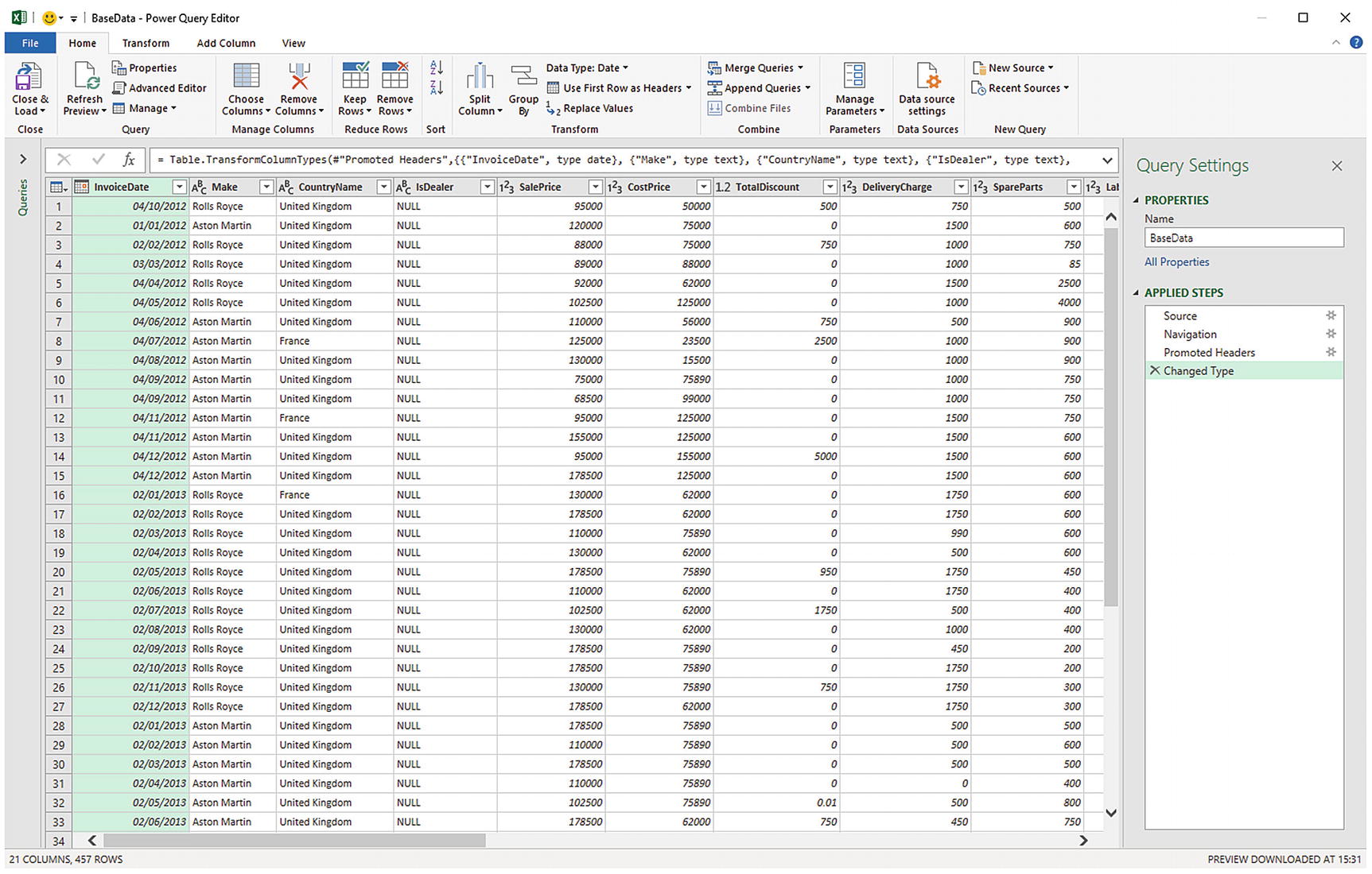
The Power Query Editor
- 5.
Right-click the title of the CostPrice column (do not click the arrow to the right of the column). The column will be selected.
- 6.
Select Rename from the context menu. You can see the context menu in Figure 6-3.
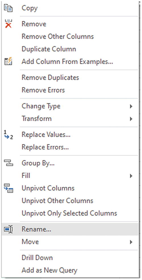
The column context menu in the Query Editor
- 7.
Type VehicleCost and press Enter. The column title will change to VehicleCost.
- 8.
In the Power Query Editor Home ribbon, click the Close & Load button. The Power Query Editor will close and return you to Excel where the source data has been loaded into a new worksheet.
I hope that this simple example makes it clear that transforming the source data is a quick and painless process. The technique that you applied—renaming a column—is only one of many dozens of possible techniques that you can apply to transform your data. However, it is not the specific transformation that is the core idea to take away here. What you need to remember is that the data that underpins your analytics is always present and it is only a click away. At any time, you can “flip” to the data and make changes, simply by double-clicking the relevant query in the Queries & Connections pane. Any changes that you make and confirm will update your data in Excel almost instantaneously.
Transforming Data Before Loading
- 1.
Open a new Excel workbook.
- 2.
In the Data ribbon, click the tiny triangle in the Get Data button.
- 3.
Select From File ➤ From Workbook and click Import for the Excel file C:DataMashupWithExcelSamplesCarSales.xlsx.
- 4.
In the Navigator window, select the CarData worksheet.
- 5.
Click the Transform data button (not the Load button).
- 6.
The Power Query Editor will open and display the source data as a table.
- 7.
Carry out steps 4 through 6 from the previous example to rename the CostPrice column.
- 8.
In the Power Query Editor Home ribbon, click the Close & Load button. The Power Query Editor will close and return you to the Excel window.
This time, you have made a simple modification to the data before loading the dataset into Excel. The data modification technique was exactly the same. The only difference between loading the data directly and taking a detour via Power Query was clicking Edit Data instead of Load in the Navigator dialog. This means that the data was only loaded once you had finished making any modifications to the source data in the Power Query Editor.
Query or Load?
Are you convinced that the data is ready to use? That is, is it clean and well structured? If so, then you can try loading it directly into Excel.
Are you faced with multiple data sources that need to be combined and molded into a coherent structure? If this is the case, then you really need to transform the data using the Power Query Editor.
Does the data come from an enterprise data warehouse or a coherently structured external source? This could be held in a relational database, a SQL Server Analysis Services cube, an in-memory tabular data warehouse, or a cloud-based service. As these data sources are nearly always the result of many hundreds—or even thousands—of hours of work cleansing, preparing, and structuring the data, you can probably load these straight into the data model or an Excel worksheet.
Does the data need to be preaggregated and filtered? Think Power Query.
Are you likely to need to change the field names to make the data more manageable? It could be simpler to change the field names in the Query Editor.
Are you faced with lots of lookup tables that need to be added to a “core” data table? Then Power Query is your friend.
Does the data contain many superfluous or erroneous elements? Then use Power Query to remove these as a first step.
Does the data need to be rationalized and standardized to make it easier to handle? In this case, the path to success is via the Power Query Editor.
Is the data source enormous? If this is the case, you could save time by editing and subsetting and filtering the data first in the Power Query Editor. This is because the Power Query Editor only loads a sample of the data for you to tweak. The entire dataset will only be loaded when you confirm all your modifications and close the Query Editor.
These kinds of questions are only rough guidelines. Yet they can help to point you in the right direction when you are working with Power Query. Inevitably, the more that you work with this application, the more you will develop the reflexes and intuition that will help you make the correct decisions. Remember, however, that Power Query is there to help and that even a directly loaded dataset is based on a query. So you can always load data and then decide to tweak the query structure later if you need to. Alternatively, editing data in a Query window can be a great opportunity to take a closer look at your data before loading it into Excel—and it only adds a couple of clicks.
This all means that you are free to adopt a way of working that you feel happy with. Power Query will adapt to your style easily and almost invisibly, letting you switch from data to Excel so fluidly that it will likely become second nature.
The remainder of this chapter will take you through some of the core techniques that you need to know to cleanse and shape your data. However, before getting into all the detail, let’s take a quick, high-level look at the Power Query Editor and the way that it is laid out.
The Power Query Editor
All of your data transformation will take place in the Power Query Editor. It is a separate window from the Excel interface that you are used to, and it has a slightly different layout.
The four principal ribbons: Home, Transform, Add Column, and View. Other ribbons are available when carrying out specific types of data transformations.
The Query list pane containing all the queries that have been added to an Excel file.
The Data window, where you can see a sample of the data for a selected query.
The Query Settings pane that contains the list of steps used to transform data.
The formula bar above the data that shows the code (written in the “M” language that you will discover in Chapter 12) that performs the selected transformation step.
The status bar (at the bottom of the window) that indicates useful information, such as the number of rows and columns in a query table and the date when the dataset was downloaded
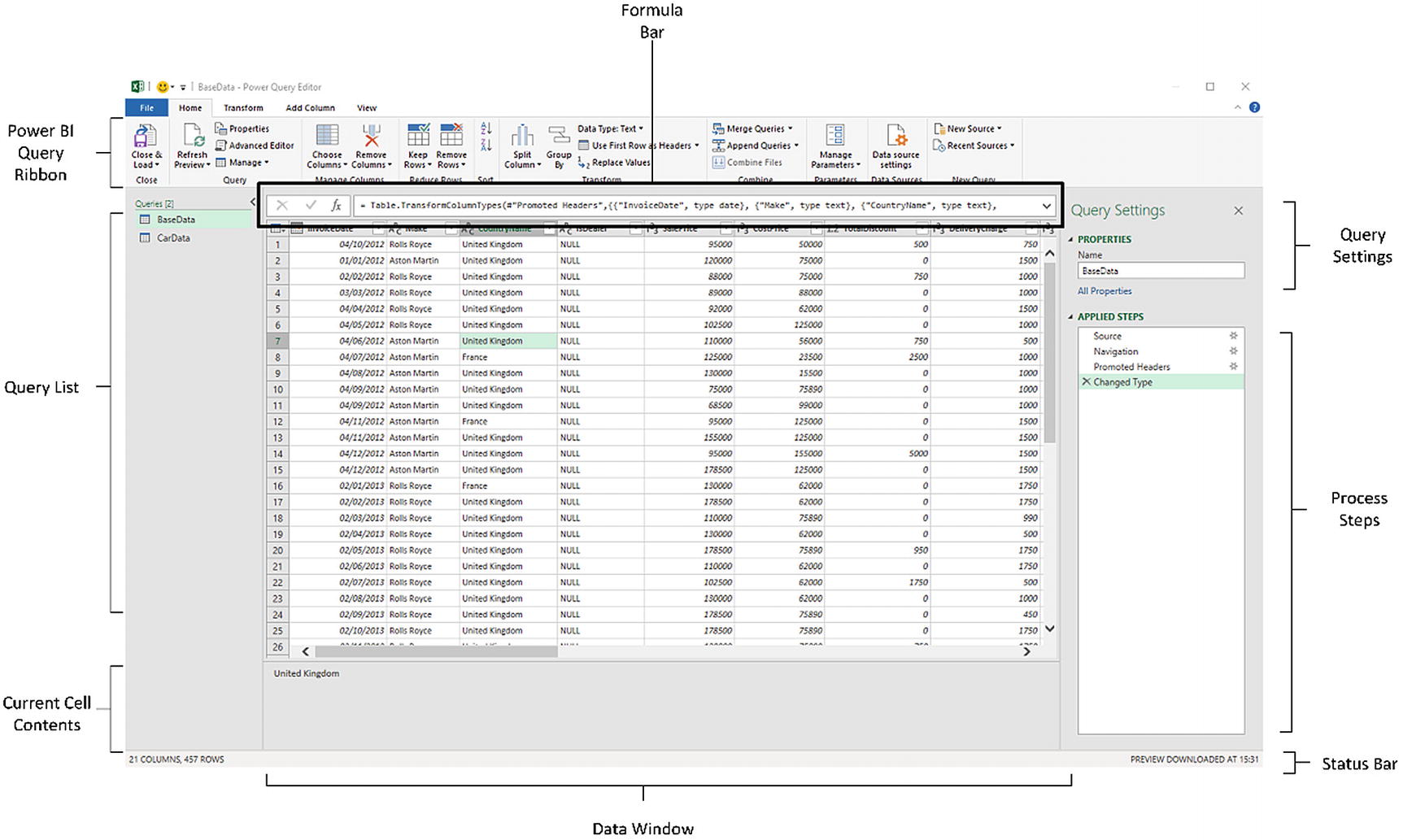
The Power Query Editor, explained
If you do not see the formula bar, just click View ➤ Formula Bar in the Power Query Editor menu.
The Applied Steps List
Data transformation is by its very nature a sequential process. So the Query window stores each modification that you make when you are cleansing and shaping source data. The various elements that make up a data transformation process are listed in the Applied Steps list of the Query Settings pane in the Power Query Editor.
The Power Query Editor does not number the steps in a data transformation process, but it certainly remembers each one. They start at the top of the Applied Steps list (nearly always with the Source step) and can extend to dozens of individual steps that trace the evolution of your data until you load it into the data model. You can, if you want, consider the Query Editor as a kind of “macro recorder.”
Moreover, as you click each step in the Applied Steps list, the data in the Data window changes to reflect the results of each transformation, giving you a complete and visible trail of all the modifications that you have applied to the dataset.
The Applied Steps list gives a distinct name to the step for each and every data modification option that you cover in this chapter and the next. As it can be important to understand exactly what each function actually achieves, I will always draw to your attention the standard name that Power Query applies.
The Power Query Editor Ribbons
The Home ribbon
The Transform ribbon
The Add Column ribbon
The View ribbon
I am not suggesting for a second that you need to memorize what all the buttons in these ribbons do. What I hope is that you are able to use the following brief descriptions of the Query Editor ribbon buttons to get an idea of the amazing power of Power Query in the field of data transformation. So if you have an initial dataset that is not quite as you need it, you can take a look at the resources that Power Query has to offer and how they can help. Once you find the function that does what you are looking for, you can jump to the relevant section for the full details on how to apply it.
The Home Ribbon
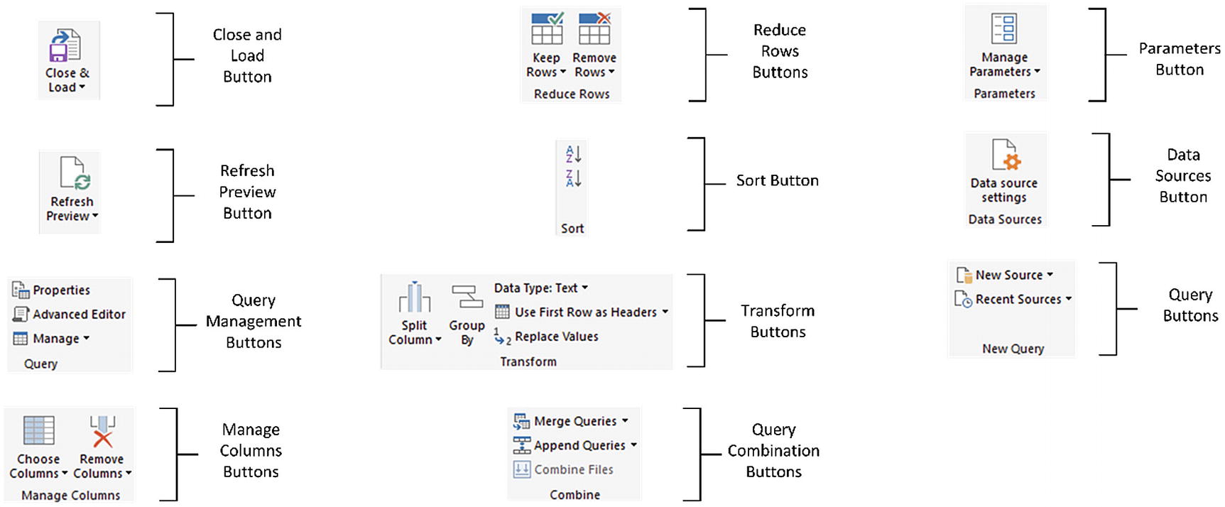
The Query Editor Home ribbon
Query Editor Home Ribbon Options
Option | Description |
|---|---|
Close & Load | Finishes the processing steps; saves and closes the query |
Refresh Preview | Refreshes the preview data |
Query Management | Lets you delete, duplicate, or reference a query |
Manage Columns | Lets you select the columns to retain from all the columns available in the source data or remove one or more columns |
Reduce Rows | Keeps or removes the specified number of rows at the top or bottom of the table |
Sort | Sorts the table using the selected column as the sort key |
Split Column | Separates the column into two or more separate columns |
Group By | Groups and potentially aggregates the data |
Data Type | Sets the column data type |
Use First Row as Headers | Promotes the first record as the header definitions |
Replace Values | Replaces values in a column with other values |
Merge Queries | Joins data from two separate queries |
Append Queries | Adds data from one or more queries into another identically structured query |
Combine Files | Merges all files in a given column into a single table |
Manage Parameters | Lets you view and modify any parameters defined for this ETL process in Power Query |
Data Source Settings | Allows you to manage and edit settings for data sources that you have already connected to |
New Query | Allows you to connect to additional external data or reuse existing connections |
The Transform Ribbon
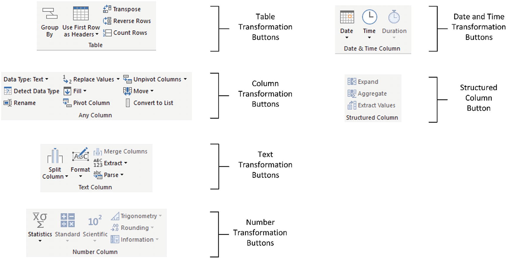
The Query Editor Transform ribbon
Query Editor Transform Ribbon Options
Option | Description |
|---|---|
Group By | Groups the table using a specified set of columns; aggregates any numeric columns for this grouping |
Use First Row As Headers | Uses the first row as the column titles |
Transpose | Transforms the columns into rows and the rows into columns |
Reverse Rows | Displays the source data in reverse order, showing the final rows at the top of the window |
Count Rows | Counts the rows in the table and replaces the data with the row count |
Data Type | Applies the chosen data type to the column |
Detect Data Type | Detects the correct data type to apply to multiple columns |
Rename | Renames a column |
Replace Values | Carries out a search-and-replace operation inside a column, replacing a specified value with another value |
Fill | Copies the data from cells above or below into empty cells in the column |
Pivot Column | Creates a new set of columns using the data in the selected column as the column titles |
Unpivot Columns | Takes the values in a set of columns and unpivots the data, creating new columns using the column headers as the descriptive elements |
Move | Moves a column |
Convert to List | Converts the contents of a column to a list. This can be used, for instance, as query parameters |
Split Column | Splits a column into one or many columns at a specified delimiter or after a specified number of characters |
Format | Modifies the text format of data in a column (uppercase, lowercase, capitalization) or removes trailing spaces |
Merge Columns | Takes the data from several columns and places it in a single column, adding an optional separator character |
Extract | Replaces the data in a column using a defined subset of the current data. You can specify a number of characters to keep from the start or end of the column, set a range of characters beginning at a specified character, or even list the number of characters in the column |
Parse | Creates an XML or JSON document from the contents of an element in a column |
Statistics | Returns the Sum, Average, Maximum, Minimum, Median, Standard Deviation, Count, or Distinct Value Count for all the values in the column |
Standard | Carries out a basic mathematical calculation (add, subtract, divide, multiply, integer-divide, or return the remainder) using a value that you specify applied to each cell in the column |
Scientific | Carries out a basic scientific calculation (square, cube, power of n, square root, exponent, logarithm, or factorial) for each cell in the column |
Trigonometry | Carries out a basic trigonometric calculation (Sine, Cosine, Tangent, ArcSine, ArcCosine, or ArcTangent) using a value that you specify applied to each cell in the column |
Rounding | Rounds the values in the column either to the next integer (up or down) or to a specified factor |
Information | Replaces the value in the column with simple information: Is Odd, Is Even, or Positive/Negative |
Date | Isolates an element (day, month, year, etc.) from a date value in a column |
Time | Isolates an element (hour, minute, second, etc.) from a date/time or time value in a column |
Duration | Calculates the duration from a value that can be interpreted as a duration in days, hours, minutes, etc. |
Expand | Adds the (identically structured) data from another query to the current query |
Aggregate | Calculates the sum or product of numeric columns from another query and adds the result to the current query |
Extract Values | Extracts the values of the contents of a column as a single text value |
The Add Column Ribbon
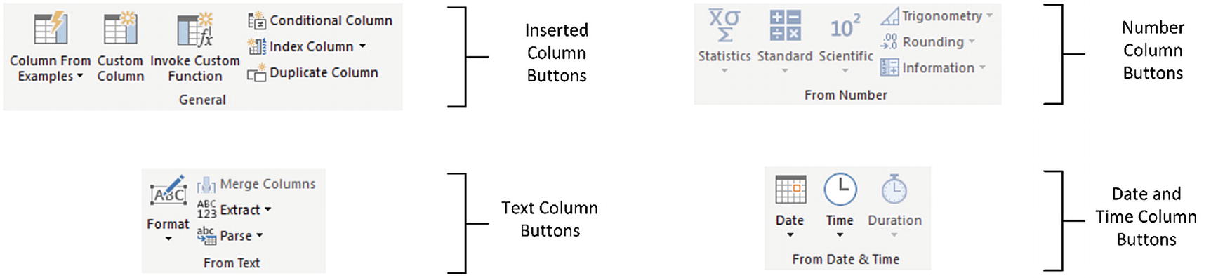
The Query Editor Add Column ribbon
Query Editor Add Column Ribbon Options
Option | Description |
|---|---|
Column From Examples | Lets you use one or more columns as examples to create a new column |
Custom Column | Adds a new column using a formula to create the column’s contents |
Invoke Custom Function | Applies an “M” language function to every row |
Conditional Column | Adds a new column that conditionally adds the values from the selected column |
Index Column | Adds a sequential number in a new column to uniquely identify each row |
Duplicate Column | Creates a copy of the current column |
Format | Modifies the text format of data in a new column (uppercase, lowercase, capitalization) or removes trailing spaces |
Merge Columns | Takes the data from several columns and places it in a single column, adding an optional separator character |
Extract | Creates a new column using a defined subset of the current data. You can specify a number of characters to keep from the start or end of the column, set a range of characters beginning at a specified character, or even list the number of characters in the column |
Parse | Creates a new column based on the XML or JSON in a column |
Statistics | Creates a new column that returns the Sum, Average, Maximum, Minimum, Median, Standard Deviation, Count, or Distinct Value Count for all the values in the column |
Standard | Creates a new column that returns a basic mathematical calculation (add, subtract, divide, multiply, integer-divide, or return the remainder) using a value that you specify applied to each cell in the column |
Scientific | Creates a new column that returns a basic scientific calculation (square, cube, power of n, square root, exponent, logarithm, or factorial) for each cell in the column |
Trigonometry | Creates a new column that returns a basic trigonometric calculation (Sine, Cosine, Tangent, ArcSine, ArcCosine, or ArcTangent) using a value that you specify applied to each cell in the column |
Rounding | Rounds the values in a new column either to the next integer (up or down) or to a specified factor |
Information | Replaces the value in the column with simple information: Is Odd, Is Even, or Positive/Negative |
Date | Isolates an element (day, month, year, etc.) from a date value in a new column |
Time | Isolates an element (hour, minute, second, etc.) from a date/time or time value in a new column |
Duration | Calculates the duration from a value that can be interpreted as a duration in days, hours, minutes, and seconds in a new column |
The View Ribbon
The View ribbon lets you alter some of the Query Editor settings and see the underlying data transformation code. The various options that it contains are explained in the next chapter.
Dataset Shaping
Renaming columns
Reordering columns
Removing columns
Merging columns
Removing records
Removing duplicate records
Filtering the dataset
I have grouped these techniques together as they affect the initial size and shape of the data. Also, it is generally not only good practice but also easier for you, the data modeler, if you begin by excluding any rows and columns that you do not need. I also find it easier to understand datasets if the columns are logically laid out and given comprehensible names from the start. All in all, this makes working with the data easier in the long run.
Renaming Columns
Although we took a quick look at renaming columns in the first pages of this chapter, let’s look at this technique again in more detail. I admit that renaming columns is not actually modifying the form of the data table. However, when dealing with data, I consider it vital to have all data clearly identifiable. This implies meaningful column names being applied to each column. Consequently, I consider this modification to be fundamental to the shape of the data and also as an essential best practice when importing source data.
- 1.
Click inside (or on the column header for) the column that you want to rename.
- 2.
Click Transform to activate the Transform ribbon.
- 3.
Click the Rename button. The column name will be highlighted.
- 4.
Enter the new name or edit the existing name.
- 5.
Press Enter or click outside the column title.
The column will now have a new title. The Applied Steps list on the right will now contain another element, Renamed Columns. This step will be highlighted.
As an alternative to using the Transform ribbon, you can right-click the column title and select Rename.
Reordering Columns
- 1.
Click the header of the column you want to move.
- 2.
Drag the column left or right to its new position. You will see the column title slide laterally through the column titles as you do this, and a thicker gray line will indicate where the column will be placed once you release the mouse button. Reordered Columns will appear in the Applied Steps list.
Reordering columns
Move Button Options
Option | Description |
|---|---|
Left | Moves the currently selected column to the left of the column on its immediate left |
Right | Moves the currently selected column to the right of the column on its immediate right |
To Beginning | Moves the currently selected column to the left of all the columns in the query |
To End | Moves the currently selected column to the right of all the columns in the query |
The Move command also works on a set of columns that you have selected by Ctrl-clicking and/or Shift-clicking. Indeed, you can move a selection of columns that is not contiguous if you need to.
You need to select a column (or a set of columns) before clicking the Move button. If you do not, then the first time that you use Move, Power Query selects the column(s) but does not move it.
Removing Columns
- 1.
Click inside the column you want to delete, or if you want to delete several columns at once, Ctrl-click the titles of the columns that you want to delete.
- 2.
Click the Remove Columns button in the Home ribbon. The column(s) will be deleted and Removed Columns will be the latest element in the Applied Steps list.
Another way to remove selected columns is to press the delete key. This will also add a “Removed Columns” step to the Applied Steps list.
- 1.
Ctrl-click the titles of the columns that you want to keep.
- 2.
Click the small triangle in the Remove Columns button in the Home ribbon. Select Remove Other Columns from the menu. All unselected columns will be deleted and Removed Other Columns will be added to the Applied Steps list.
When selecting a contiguous range of columns to remove or keep, you can use the standard Windows Shift-click technique to select from the first to the last column in the block of columns that you want to select.
Both of these options for removing columns are also available from the context menu, if you prefer. It shows Remove (or Remove Columns, if there are several columns selected) when deleting columns, as well as Remove Other Columns if you right-click a column title.
Choosing Columns
- 1.
Open the sample file Chapter06Sample1.xlsx in the folder C:DataMashupWithExcelSamples unless it is already open.
- 2.
In the Queries & Connections pane on the right (that you can toggle on and off from the Data ribbon Queries & Connections option), double-click the connection BaseData. The Query Editor will open.
- 3.
In the Home ribbon of the Query Editor, click the Choose Columns button.
- 4.
Click (Select All Columns) to deselect the entire collection of columns in the dataset.
- 5.
Select the columns Make, Model, Color, and SalePrice. The Choose Columns dialog will look like the one in Figure 6-9.
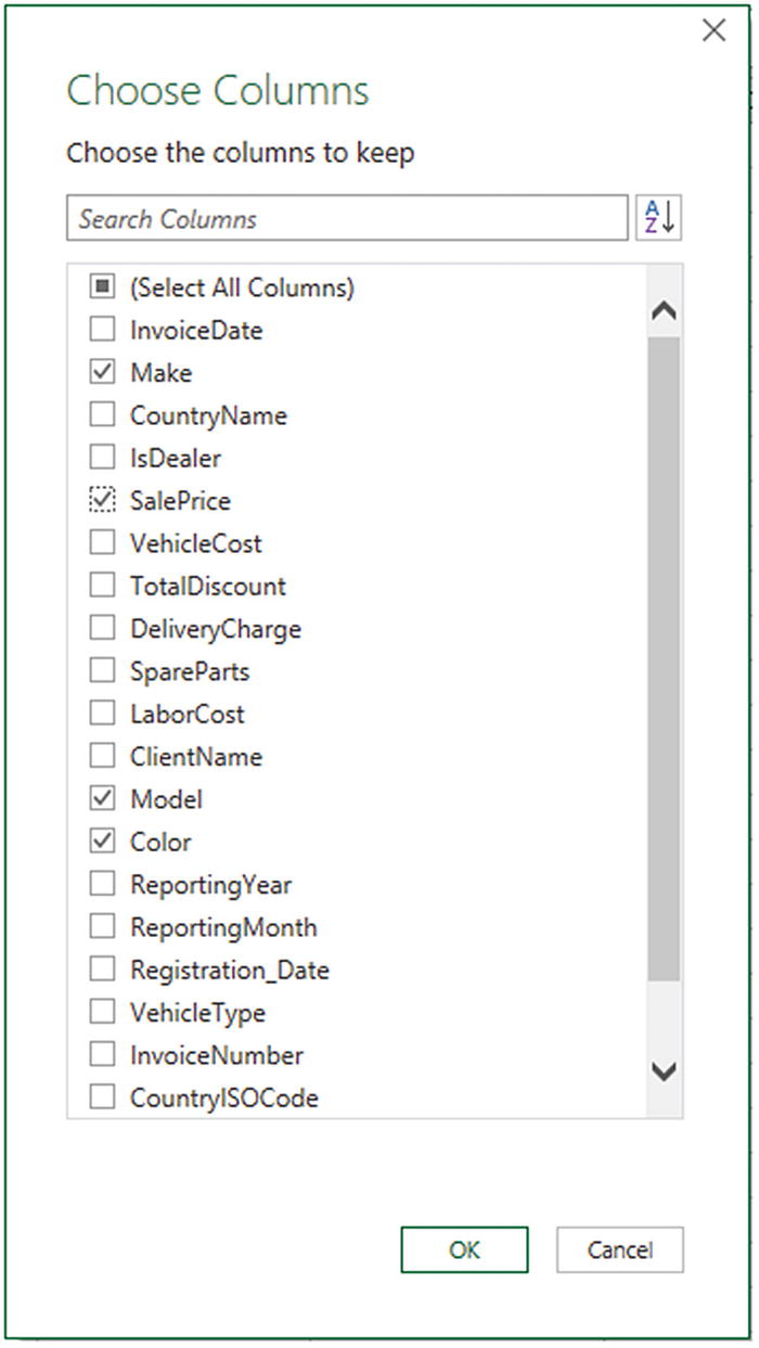
The Choose Columns dialog
- 6.
Click OK. The Query Editor will only display the columns that you selected.
You can sort the column list in alphabetical order (or, indeed, revert to the original order) by clicking the Sort icon (the small A-Z) at the top right of the Choose Columns dialog and selecting the required option.
You can filter the list of columns that is displayed simply by entering a few characters in the Search Columns field at the top of the dialog.
The (Select All Columns) option switches between selecting and deselecting all the columns in the list.
Merging Columns
- 1.
Ctrl-click the headers of the columns that you want to merge (Make and Model in the BaseData dataset in this example).
- 2.
In the Transform ribbon, click the Merge Columns button. The Merge Columns dialog will be displayed.
- 3.
From the Separator popup menu, select one of the available separator elements. I chose Colon in this example.
- 4.
Enter a name for the column that will be created from the two original columns (I am calling it MakeAndModel). The dialog should look like Figure 6-10.
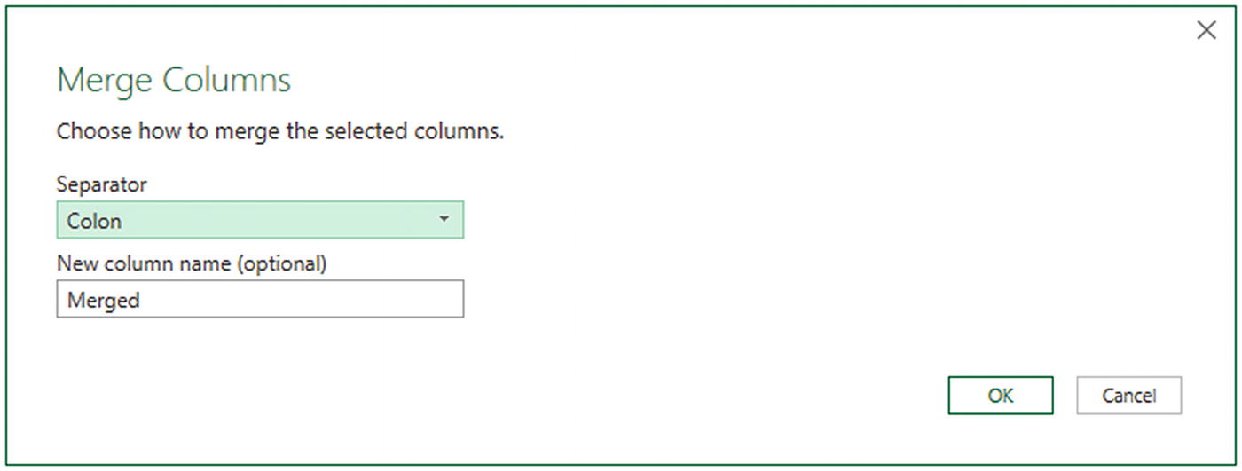
The Merge Columns dialog
- 5.
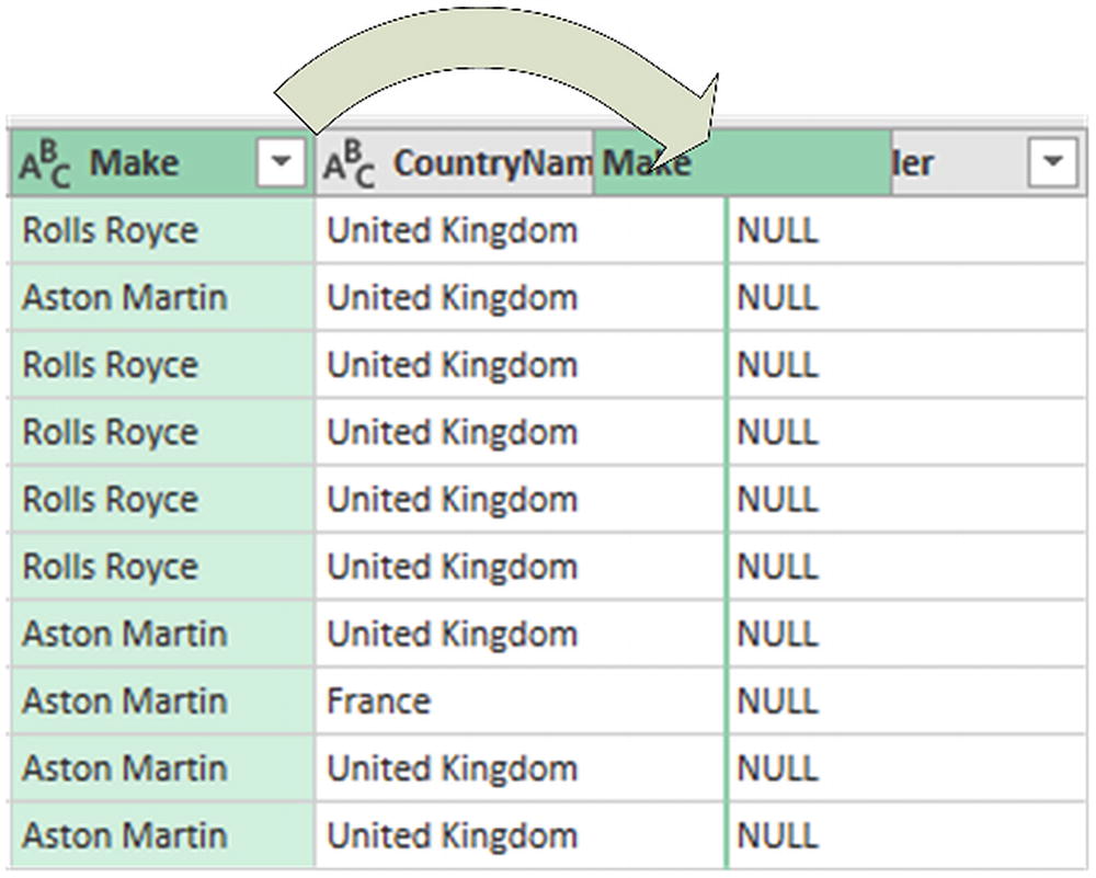
Click OK. The columns that you selected will be replaced by the data from all the columns that you selected in step 1, as shown in Figure 6-11.
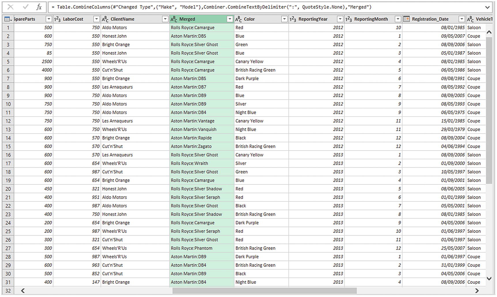
The result of merging columns
- 6.
Rename the resulting column (named Merged by Power Query).
You can select as many columns as you want when merging columns.
If you do not give the resulting column a name in the Merge Columns dialog, it will simply be renamed Merged. You can always rename it later if you want.
The order in which you select the columns affects the way that the data is merged. So, always begin by selecting the column whose data must appear at the left of the merged column, then the column whose data should be next, and so forth. You do not have to select columns in the order that they initially appeared in the dataset.
If you do not want to use any of the standard separators that Power Query suggests, you can always define your own. Just select --Custom-- in the popup menu in the Merge Columns dialog. A new box will appear in the dialog, in which you can enter your choice of separator. This can be composed of several characters if you really want.
Merging columns from the Transform ribbon removes all the selected columns and replaces them with a single column. The same option is also available from the Add Column ribbon—only in this case, this operation adds a new column and leaves the original columns in the dataset.
This option is also available from the context menu if you right-click a column title.
Merge Separators
Option | Description |
|---|---|
Colon | Uses the colon (:) as the separator |
Comma | Uses the comma (,) as the separator |
Equals Sign | Uses the equals sign (=) as the separator |
Semi-Colon | Uses the semicolon (;) as the separator |
Space | Uses the space ( ) as the separator |
Tab | Uses the tab character as the separator |
Custom | Lets you enter a custom separator |
You can split, remove, and duplicate columns using the context menu if you prefer. Just remember to right-click the column title to display the correct context menu.
Moving to a Specific Column
- 1.
In the Home ribbon of the Query Editor, click the small triangle at the bottom of the Choose Columns button. Select Go to Column. The Go to Column dialog will appear.
- 2.
Select the column you want to move to. The dialog will look like Figure 6-12.
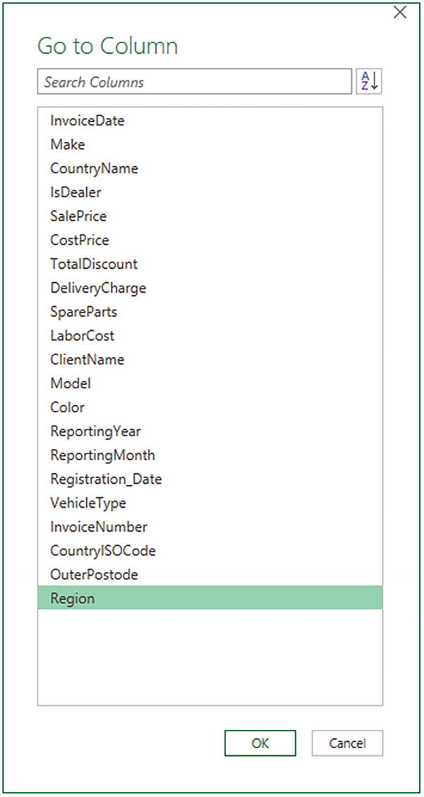
The Go to Column dialog
- 3.
Click OK. Power Query will select the chosen column.
If you prefer, you can double-click a column name in the Go to Column dialog to move to the chosen column.
Removing Records
You are taking a first look at the data, and you only need a sample to get an idea of what the data is like.
The data contains records that you clearly do not need and that you can easily identify from the start.
You are testing data cleansing and you want a smaller dataset to really speed up the development of a complex data extraction and transformation process.
You want to analyze a reduced dataset to extrapolate theses and inferences, and to save analysis on a full dataset for later, or even use a more industrial-strength toolset such as SQL Server Integration Services.
Keep certain rows
Remove certain rows
Inevitably, the technique that you adopt will depend on the circumstances. If it is easier to specify the rows to sample by inclusion, then the keep-certain-rows approach is the best option to take. Inversely, if you want to proceed by exclusion, then the remove-certain-rows technique is best. Let’s look at each of these in turn.
Keeping Rows
Keep the top n records.
Keep the bottom n records.
Keep a specified range of records—that is, keep n records every y records.
- 1.
Open the source file and then open the Power Query Editor by double-clicking the BaseData query in the Queries & Connections pane.
- 2.
In the Home ribbon of the Query Editor, click the Keep Rows button. The menu will appear.
- 3.
Select Keep Top Rows. The Keep Top Rows dialog will appear.
- 4.
Enter 50 in the “Number of rows” box, as shown in Figure 6-13.
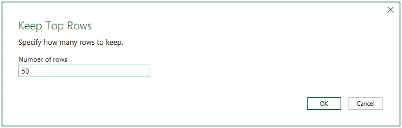
The Keep Top Rows dialog
- 5.
Click OK. All but the first 50 records are deleted and Kept First Rows is added to the Applied Steps list.
To keep the bottom n rows, the technique is virtually identical. Follow the steps in the previous example, but select Keep Bottom Rows in step 2. In this case, the Applied Steps list displays Kept Last Rows.
- 1.
In the Home ribbon, click the Keep Rows button.
- 2.
Select Keep Range of Rows. The Keep Range of Rows dialog will appear.
- 3.
Enter 11 in the “First row” box.
- 4.
Enter 25 in the “Number of rows” box, as shown in Figure 6-14.
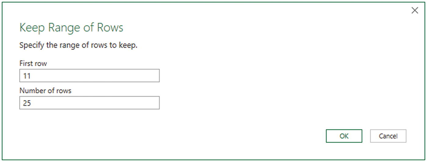
The Keep Range of Rows dialog
- 5.
Click OK. All but records 1–10 and 36 to the end are deleted and Kept Range of Rows is added to the Applied Steps list.
Removing Rows
Removing rows is a nearly identical process to the one you just used to keep rows. As removing the top or bottom n rows is highly similar, I will not go through it in detail. All you have to do is click the Remove Rows button in the Home ribbon and follow the process as if you were keeping rows. The Applied Steps list will read Removed Top Rows or Removed Bottom Rows in this case, and rows will be removed instead of being kept in the dataset, of course.
- 1.
Click the Remove Rows button in the Query window Home ribbon. The menu will appear.
- 2.
Select Remove Alternate Rows. The Remove Alternate Rows dialog will appear.
- 3.
Enter 10 as the First row to remove.
- 4.
Enter 2 as the Number of rows to remove.
- 5.
Enter 10 as the Number of rows to keep.
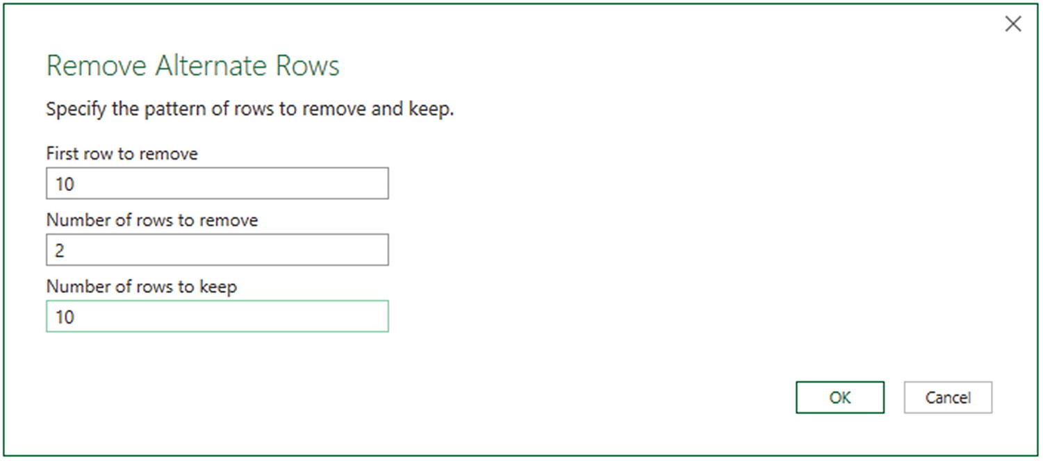
The Remove Alternate Rows dialog
- 6.
Click OK. All but the records matching the pattern you entered in the dialog are removed. Removed Alternate Rows is then added to the Applied Steps list.
If you are really determined to extract a sample that you consider to be representative of the key data, then you can always filter the data before subsetting it to exclude any outliers. Filtering data is explained later in this chapter.
Removing Blank Rows
- 1.
Click the Remove Rows button in the Query window Home ribbon. The menu will appear.
- 2.
Select Remove Blank Rows.
This results in empty rows being deleted. Removed Blank Rows is then added to the Applied Steps list.
Removing Duplicate Records
- 1.
Click the Remove Duplicates in the popup menu for the table (this is at the top left of the table grid). All duplicate records are deleted and Removed Duplicates is added to the Applied Steps list.
I must stress that this approach will only remove completely identical records where every element of every column is strictly identical in the duplicate rows. If two records have just one different character or a number but everything else is identical, then they are not considered duplicates by Power Query. Alternatively, if you want to isolate and examine the duplicate records, then you can display only completely identical records by selecting Keep Duplicates from the popup menu for the table.
Remove all columns that you are sure you will not be using later in the data-handling process. This way, Power Query will only be asked to compare essential data across potentially duplicate records.
Group the data on the core columns (this is explained later in this chapter).
As you have seen, Power Query can help you to home in on the essential elements in a dataset in just a few clicks. If anything, you need to be careful that you are not removing valuable data—and consequently skewing your analysis—when excluding data from the query.
Sorting Data
- 1.
Open the sample file Chapter06Sample1.xlsx in the folder C:DataMashupWithExcelSamples unless it is already open.
- 2.
In the Queries & Connections pane on the right, double-click the connection BaseData. The Query Editor will open.
- 3.
Click inside the column you wish to sort by.
- 4.
Click Sort Ascending (the A/Z icon) or Sort Descending (the Z/A icon) in the Home ribbon.
Sorting multiple columns
If you look closely at the column headings, you will see a small “1” and “2” that indicate the sort priority as well as the arrows that indicate that the columns are sorted in ascending order.
An alternative technique for sorting data is to click the popup menu for a column (the downward-facing triangle at the right of a column title) and select Sort Ascending or Sort Descending from the popup menu.
Reversing the Row Order
If you find that the data that you are looking at seems upside down (i.e., with the bottom rows at the top and vice versa), you can reverse the row order in a single click, if you want. To do this, do the following:
In the Transform ribbon, click the Reverse Rows button.
The entire dataset will be reversed and the bottom row will now be the top row.
Undoing a Sort Operation
If you subsequently decide that you do not want to keep your data sorted, you can undo the sort operation at any time, as follows:
- 1.
Click the sort icon at the right of the name of the column that you used as the basis for the sort operation. The context menu will appear, as you can see in Figure 6-17.
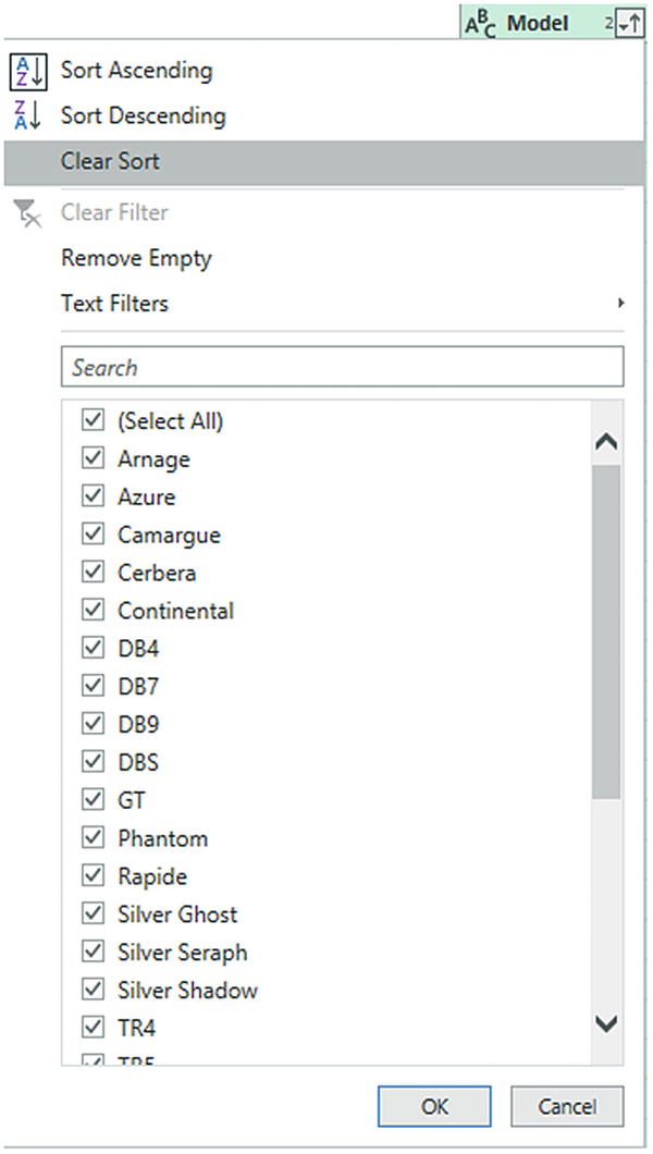
Removing a sort operation
- 2.
Click Clear Sort.
The sort order that you applied will be removed, and the data will revert to its original row order.
As sorting data is considered part of the data modification process, it also appears in the Applied Steps list as Sorted Rows. This means that you can also remove a sort operation by deleting the relevant step in the Applied Steps list.
If you sorted the dataset on several columns, you can choose to remove all the sort order that you applied by clicking the first column that you used to sort the data. This will remove the sort order that you applied to all the columns that you used to define the sort criteria. If all you want to do is undo the sort on the final column in a set of columns used to sort the recordset, then you can clear only the sort operation on this column.
Filtering Data
The most frequently used way of limiting a dataset is, in my experience, the use of filters on the table that you have loaded. Now, I realize that you may be coming to Power Query after years with Excel, or after some time using Power Pivot, and that the filtering techniques that you are about to see probably look much like the ones you have used in those two tools. However, because it is fundamental to include and exclude appropriate records when loading source data, I prefer to explain Power Query filters in detail, even if this means that certain readers will experience a strong sense of déjà vu.
Select one or more specific values from the unique list of elements in the chosen column.
Define a range of data to include or exclude.
The first option is common to all data types, whether they are text, number, or date/time. The second approach varies according to the data type of the column that you are using to filter data.
Selecting Specific Text Values
- 1.
Click a column’s popup menu. (I used Make in the sample dataset Chapter06Sample1.xlsx here.) The filter menu appears.
- 2.
Check all elements that you want to retain and uncheck all elements that you wish to exclude. In this example, I kept Bentley and Rolls Royce, as shown in Figure 6-18.
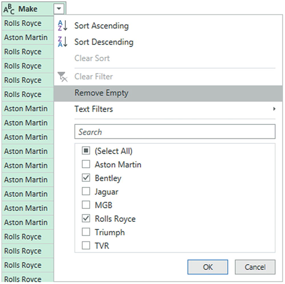
A filter menu
- 3.
Click OK. Filtered Rows is added to the Applied Steps list.
You can deselect all items by clicking the (Select All) check box; reselect all the items by selecting this box again. It follows that if you want to keep only a few elements, it may be faster to unselect all of them first and then only select the ones that you want to keep. If you want to exclude any records without a value in the column that you are filtering on, then select Remove Empty from the filter menu.
Finding Elements in the Filter List
- 1.
Click the popup menu for a column. (I use Model in the sample dataset in this example.) The filter menu appears.
- 2.
Enter a letter or a few letters in the Search box. The list shortens with every letter or number that you enter. If you enter ar, then the filter popup will look like Figure 6-19.
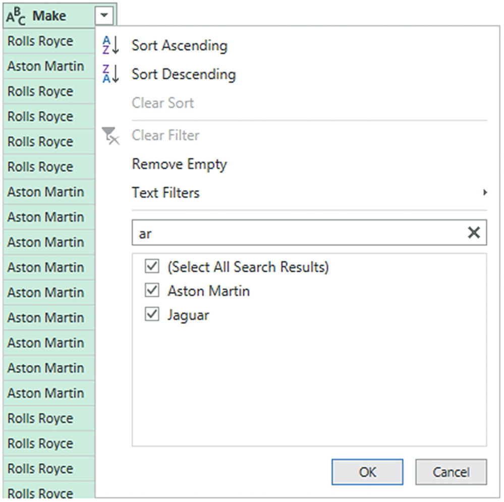
Searching the filter menu
- 3.
Select the elements that you want to filter on and click OK.
To remove a filter, all that you have to do is click the cross that appears at the right of the Search box.
Filtering Text Ranges
Text Filter Options
Filter Option | Description |
|---|---|
Equals | Sets the text that must match the cell contents |
Does Not Equal | Sets the text that must not match the cell contents |
Begins With | Sets the text at the left of the cell contents |
Does Not Begin With | Sets the text that must not appear at the left of the cell contents |
Ends With | Sets the text at the right of the cell contents |
Does Not End With | Sets the text that must not appear at the right of the cell contents |
Contains | Lets you enter a text that will be part of the cell contents |
Does Not Contain | Lets you enter a text that will not be part of the cell contents |
Filtering Numeric Ranges
Numeric Filter Options
Filter Option | Description |
|---|---|
Equals | Sets the number that must match the cell contents |
Does Not Equal | Sets the number that must not match the cell contents |
Greater Than | Cell contents must be greater than this number |
Greater Than Or Equal To | Cell contents must be greater than or equal to this number |
Lesser Than | Cell contents must be less than this number |
Lesser Than Or Equal To | Cell contents must be less than or equal to this number |
Between | Cell contents must be between the two numbers that you specify |
Filtering Date and Time Ranges
Date and Time Filter Options
Filter Element | Description |
|---|---|
Equals | Filters data to include only records for the selected date |
Before | Filters data to include only records up to the selected date |
After | Filters data to include only records after the selected date |
Between | Lets you set an upper and a lower date limit to exclude records outside that range |
In the Next | Lets you specify a number of days, weeks, months, quarters, or years to come |
In the Previous | Lets you specify a number of days, weeks, months, quarters, or years up to the date |
Is Earliest | Filters data to include only records for the earliest date |
Is Latest | Filters data to include only records for the latest date |
Is Not Earliest | Filters data to include only records for dates not including the earliest date |
Is Not Latest | Filters data to include only records for dates not including the latest date |
Day ➤ Tomorrow | Filters data to include only records for the day after the current system date |
Day ➤ Today | Filters data to include only records for the current system date |
Day ➤ Yesterday | Filters data to include only records for the day before the current system date |
Week ➤ Next Week | Filters data to include only records for the next calendar week |
Week ➤ This Week | Filters data to include only records for the current calendar week |
Week ➤ Last Week | Filters data to include only records for the previous calendar week |
Month ➤ Next Month | Filters data to include only records for the next calendar month |
Month ➤ This Month | Filters data to include only records for the current calendar month |
Month ➤ Last Month | Filters data to include only records for the previous calendar month |
Month ➤ Month Name | Filters data to include only records for the specified calendar month |
Quarter ➤ Next Quarter | Filters data to include only records for the next quarter |
Quarter ➤ This Quarter | Filters data to include only records for the current quarter |
Quarter ➤ Last Quarter | Filters data to include only records for the previous quarter |
Quarter ➤ Quarter Name | Filters data to include only records for the specified quarter |
Year ➤ Next Year | Filters data to include only records for the next year |
Year ➤ This Year | Filters data to include only records for the current year |
Year ➤ Last Year | Filters data to include only records for the previous year |
Year ➤ Year To Date | Filters data to include only records for the calendar year to date |
Custom Filter | Lets you set up a specific filter for a chosen date range. |
Filtering Numeric Data
- 1.
Click the popup menu for the SalePrice column.
- 2.
Click Number Filters. The submenu will appear.
- 3.
Select Less Than. The Filter Rows dialog will be displayed.
- 4.
Enter 5000 in the box next to the “is less than” box, as shown in Figure 6-20.
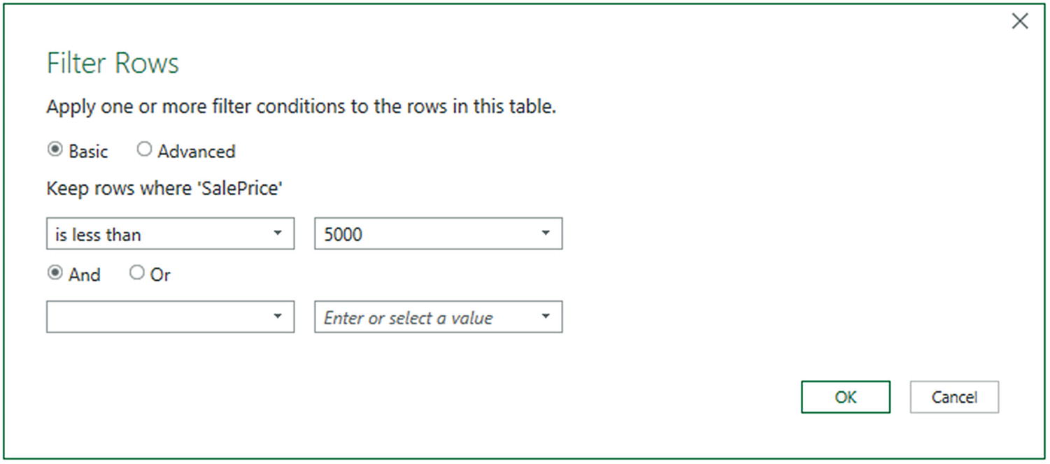
The Filter Rows dialog
- 5.
Click OK. The dataset only displays rows that conform to the filter that you have defined.
You can combine up to two elements in a basic filter. These can be mutually inclusive (an AND filter) or they can be an alternative (an OR filter).
You can combine several elements in an advanced filter—as you will learn in the next section.
You should not apply any formatting when entering numbers.
Any text that you filter on is not case-sensitive.
If you choose the wrong type of filter (for instance, greater than rather than less than), you do not have to cancel and start over. Simply select the correct filter type from the popup in the left-hand boxes in the Filter Rows dialog.
If you set a filter value that excludes all the records in the table, Power Query displays an empty table except for the words “This table is empty.” You can always remove the filter by clicking the cross to the left of Filtered Rows in the Applied Steps list. This will remove the step and revert the data to its previous state.
Applying Advanced Filters
- 1.
Click the popup menu for the SalePrice column.
- 2.
Click Number Filters. The submenu will appear.
- 3.
Select Equals. The Filter Rows dialog will be displayed.
- 4.
Click Advanced.
- 5.
Enter 5000 as the value for the first filter element in the dialog.
- 6.
Select Or from the popup as the filter type for the second filter element.
- 7.
Select equals as the operator.
- 8.
Enter 89000 as the value for the second filter in the dialog.
- 9.
Click Add Clause. A new filter element will be added to the dialog under the existing elements.
- 10.
Select Or as the filter type and equals as the operator.
- 11.
Enter 178500 as the value for the third filter element in the dialog. The Filter Rows dialog will look like the one shown in Figure 6-21.
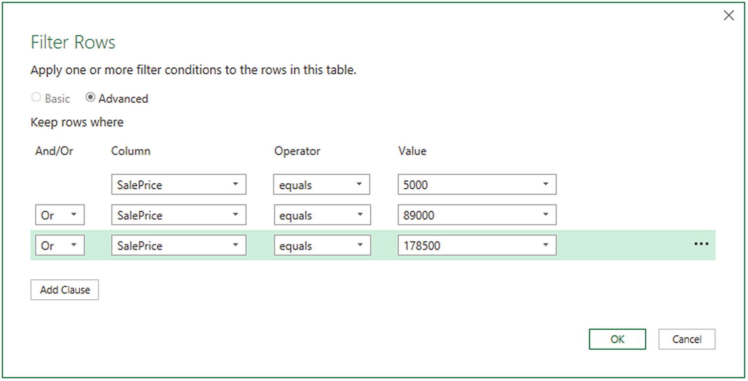
Advanced filters
- 12.
Click OK. Only records containing the figures that you entered in the Filter Rows dialog will be displayed in the Power Query Editor.
In the Advanced filter dialog, you can “mix and match” columns and operators to achieve the filter result that you are looking for.
You can also order the sequence of filters if you ever need to. To do this, simply click inside a filter row and it will appear with a gray background (like the third filter in Figure 6-21). Then click the ellipses at the right of the filter row and select Move Up or Move Down from the popup menu. You can see this in Figure 6-22.
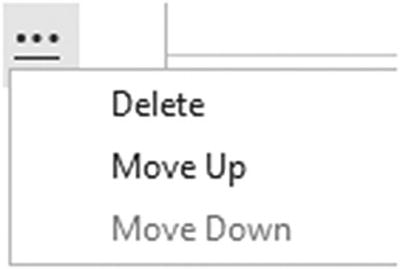
Ordering filters
To delete a filter, click the ellipses at the right of the filter row and select Delete.
When you are dealing with really large datasets, you may find that a filter does not always show all the available values from the source data. This is because the Query Editor has loaded only a sample subset of the data. In cases like these, you will see an alert in the filter popup menu and a “Load more” link. Clicking this link will force Power Query to reload a larger sample set of data. However, memory restrictions may prevent it from loading all the data that you need. In cases like this, you should consider modifying the source query (if this is possible, of course, such as when connecting to a database) so that it brings back a representative dataset that can fit into memory.
Grouping Records
Define the attribute columns that will become the unique elements in the grouped data table
Specify which aggregations are applied to any numeric columns included in the grouped table
Grouping is frequently an extremely selective operation. This is inevitable, since the fewer attribute (i.e., nonnumeric) columns you choose to group on, the fewer records you are likely to include in the grouped table. However, this will always depend on the particular dataset you are dealing with, and grouping data efficiently is always a matter of flair, practice, and good, old-fashioned trial and error.
Simple Groups
- 1.
In Power Query for the sample file Chapter06Sample1.xlsx, click inside the Make column.
- 2.
In either the Home ribbon or Transform ribbon, click the Group By button. The Group By dialog will appear, looking like the one in Figure 6-23.
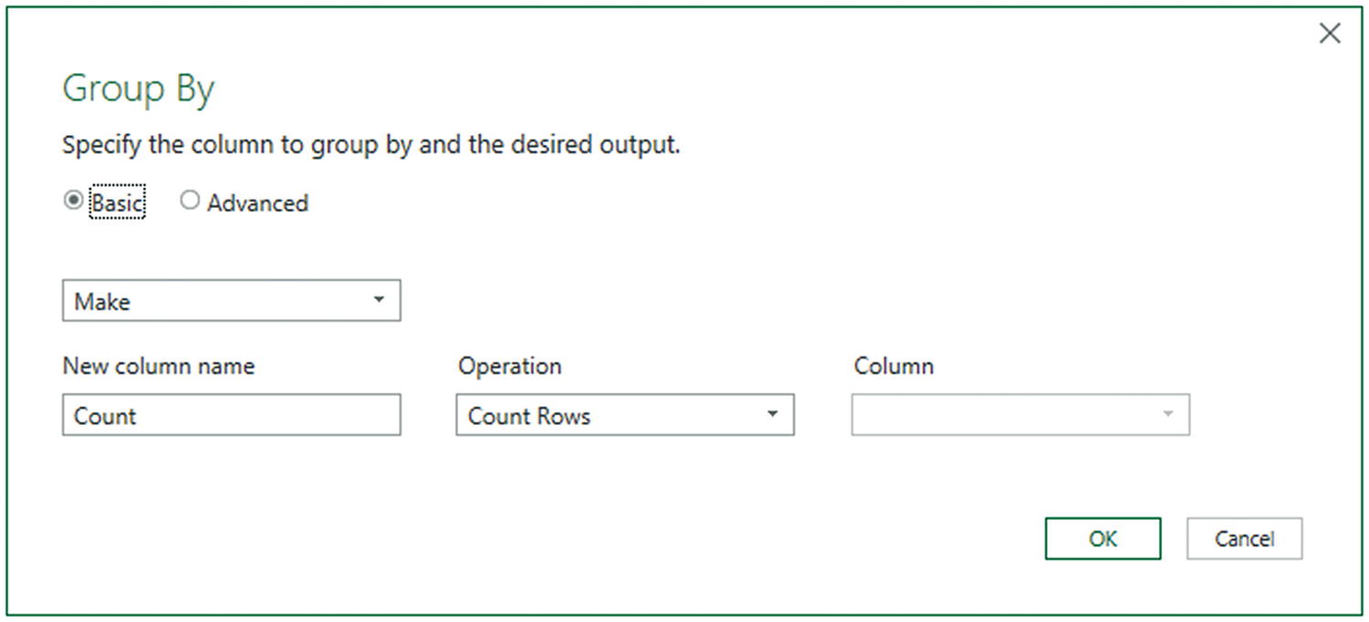
Simple grouping
- 3.
Click OK. The dataset will now only contain the list of makes of vehicle and the number of records for each make. You can see this in Figure 6-24.
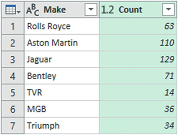
Simple grouping output
Power Query will add a step named Grouped Rows to the Applied Steps list when you apply grouping to a dataset.
The best way to cancel a grouping operation is to delete the Grouped Rows step in the Applied Steps list.
Aggregation Operations When Grouping
Aggregation Operation | Description |
|---|---|
Count Rows | Counts the number of records |
Count Distinct Rows | Counts the number of unique records |
Sum | Returns the total for a numeric column |
Average | Returns the average for a numeric column |
Median | Returns the median value of a numeric column |
Min | Returns the minimum value of a numeric column |
Max | Returns the maximum value of a numeric column |
All Rows | Creates a table of records for each grouped element |
Complex Groups
- 1.
Open the sample file C:DataMashupWithExcelSamplesChapter06Sample1.xlsx.
- 2.
Double-click the BaseData Connection to open the Query Editor.
- 3.Select the following columns (by Ctrl-clicking the column headers):
- a.
Make
- b.
Model
- a.
- 4.
In either the Home ribbon or Transform ribbon, click Group By.
- 5.
In the New Column Name box, enter TotalSales.
- 6.
Select Sum as the operation.
- 7.
Choose SalePrice as the source column in the Column popup list.
- 8.Click the Add Aggregation button and repeat the operation, only this time, use the following:
- a.
New Column Name: AverageCost
- b.
Operation: Average
- c.
Column: CostPrice
- a.

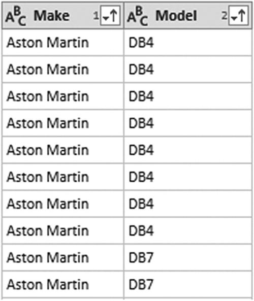
- 9.
Click OK. All columns, other than those that you specified in the Group By dialog, are removed, and the table is grouped and aggregated, as shown in Figure 6-26. Grouped Rows will be added to the Applied Steps list. I have also sorted the table by the Make and Model columns to make the grouping easier to comprehend.
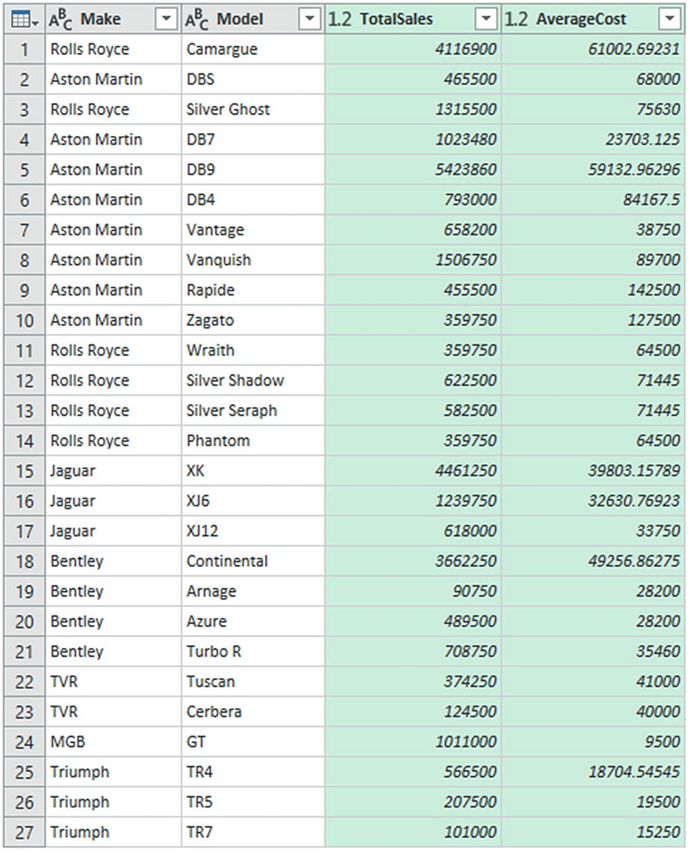
Grouping a dataset
If you have created a really complex group and then realized that you need to change the order of the columns, all is not lost. You can alter the order of the columns in the output by clicking the ellipses to the right of each column definition in the Group By dialog and selecting Move Up or Move Down. The order of the columns in the Group By dialog will be the order of the columns (left to right) in the resulting dataset.
You do not have to Ctrl-click to select the grouping columns. You can add them one by one to the Group By dialog by clicking the Add Aggregation button. Equally, you can remove grouping columns (or added and aggregated columns) by clicking the ellipses to the right of a column name and selecting Delete from the popup menu.
Count Rows
- 1.
In the Power Query Transform menu, click Count rows. The number of records will appear in the place of the existing dataset as shown in Figure 6-27.
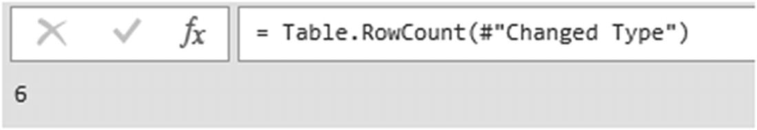
Returning the row count of a source dataset
Saving Changes in the Query Editor
Contrary to what you might expect, you cannot save any changes that you have made when using the Power Query Editor at any time. Instead you must first exit the Query Editor and then save the underlying Excel file as you would normally.
Exiting the Query Editor
In a similar vein to the Save options just described, you can choose how to exit the Query Editor and return to your reports in Excel. The default option (when you click the Close & Load button) is to apply all the changes that you have made to the data, update the data model with the new data (if this option has been selected), and return to Excel.
- 1.
In the Query Editor, click File.
- 2.
Select Discard & Close. You can see this option in Figure 6-28.
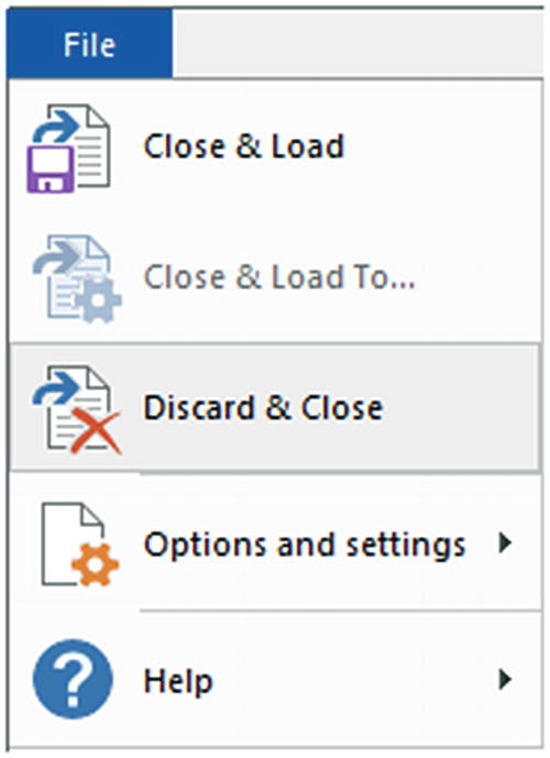
Discard modifications in Power Query
If you choose not to apply the changes that you have made, then you will return to the Excel workbook and lose any modifications you have made—without any confirmation.
Conclusion
This chapter started you on the road to transforming datasets with Power Query. You saw how to trim datasets by removing rows and columns. You also learned how to subset a sample of data from a data source by selecting alternating groups of rows.
You also saw how to choose the columns that you want to use in Excel, how to move columns around in the dataset, and how to rename columns so that your data is easily comprehensible when you use it later as the basis for your analysis. Then, you saw how to filter and sort data, as well as how to remove duplicates to ensure that your dataset only contains the precise rows that you need for your upcoming visualizations. Finally, you learned how to group and aggregate data.
It has to be admitted, nonetheless, that preparing raw data for use in analytics is not always easy and can take a while to get right. However, Power Query can make this task really easy with a little practice. So now that you have grasped the basics, it is time to move on and discover some further data transformation techniques. Specifically, you will see how to transform and potentially cleanse the data that you have imported. This is the subject of the next chapter.