- Running DAGs at regular intervals
- Constructing dynamic DAGs to process data incrementally
- Loading and reprocessing past data sets using backfilling
- Applying best practices for reliable tasks
In the previous chapter, we explored Airflow’s UI and showed you how to define a basic Airflow DAG and run it every day by defining a scheduled interval. In this chapter, we will dive a bit deeper into the concept of scheduling in Airflow and explore how this allows you to process data incrementally at regular intervals. First, we’ll introduce a small use case focused on analyzing user events from our website and explore how we can build a DAG to analyze these events at regular intervals. Next, we’ll explore ways to make this process more efficient by taking an incremental approach to analyzing our data and understanding how this ties into Airflow’s concept of execution dates. Finally, we’ll finish by showing how we can fill in past gaps in our data set using backfilling and discussing some important properties of proper Airflow tasks.
3.1 An example: Processing user events
To understand how Airflow’s scheduling works, we’ll first consider a small example. Imagine we have a service that tracks user behavior on our website and allows us to analyze which pages users (identified by an IP address) accessed. For marketing purposes, we would like to know how many different pages users access and how much time they spend during each visit. To get an idea of how this behavior changes over time, we want to calculate these statistics daily, as this allows us to compare changes across different days and larger time periods.
For practical reasons, the external tracking service does not store data for more than 30 days, so we need to store and accumulate this data ourselves, as we want to retain our history for longer periods of time. Normally, because the raw data might be quite large, it would make sense to store this data in a cloud storage service such as Amazon’s S3 or Google’s Cloud Storage, as they combine high durability with relatively low costs. However, for simplicity’s sake, we won’t worry about these things and will keep our data locally.
To simulate this example, we have created a simple (local) API that allows us to retrieve user events. For example, we can retrieve the full list of available events from the past 30 days using the following API call:
curl -o /tmp/events.json http://localhost:5000/events
This call returns a (JSON-encoded) list of user events we can analyze to calculate our user statistics.
Using this API, we can break our workflow into two separate tasks: one for fetching user events and another for calculating the statistics. The data itself can be downloaded using the BashOperator, as we saw in the previous chapter. For calculating the statistics, we can use a PythonOperator, which allows us to load the data into a Pandas DataFrame and calculate the number of events using a groupby and an aggregation. Altogether, this gives us the DAG shown in listing 3.1.
Listing 3.1 Initial (unscheduled) version of the event DAG (dags/01_unscheduled.py)
import datetime as dt
from pathlib import Path

import pandas as pd
from airflow import DAG
from airflow.operators.bash import BashOperator
from airflow.operators.python import PythonOperator

dag = DAG(
   dag_id="01_unscheduled",
   start_date=dt.datetime(2019, 1, 1),                            ❶
   schedule_interval=None,                                        ❷
)

fetch_events = BashOperator(
   task_id="fetch_events",
   bash_command=(
      "mkdir -p /data && "
      "curl -o /data/events.json "
      "http://localhost:5000/events"                            ❸
   ),
   dag=dag,
)


def _calculate_stats(input_path, output_path):
   """Calculates event statistics."""
   events = pd.read_json(input_path)                              ❹
   stats = events.groupby(["date", "user"]).size().reset_index()  ❹
   Path(output_path).parent.mkdir(exist_ok=True)                  ❺
   stats.to_csv(output_path, index=False)                         ❺


calculate_stats = PythonOperator(
   task_id="calculate_stats",
   python_callable=_calculate_stats,
   op_kwargs={
       "input_path": "/data/events.json",
       "output_path": "/data/stats.csv",
   },
   dag=dag,
)

fetch_events >> calculate_stats                                   ❻
❶ Define the start date for the DAG.
❷ Specify that this is an unscheduled DAG.
❸ Fetch and store the events from the API.
❹ Load the events and calculate the required statistics.
❺ Make sure the output directory exists and write results to CSV.
Now we have our basic DAG, but we still need to make sure it’s run regularly by Airflow. Let’s get it scheduled so that we have daily updates!
3.2 Running at regular intervals
As we saw in chapter 2, Airflow DAGs can be run at regular intervals by defining a scheduled interval for it using the schedule_interval argument when initializing the DAG. By default, the value of this argument is None, which means the DAG will not be scheduled and will be run only when triggered manually from the UI or the API.
3.2.1 Defining scheduling intervals
In our example of ingesting user events, we would like to calculate statistics daily, so it would make sense to schedule our DAG to run once every day. As this is a common use case, Airflow provides the convenient macro @daily for defining a daily scheduled interval, which runs our DAG once every day at midnight.
Listing 3.2 Defining a daily schedule interval (dags/02_daily_schedule.py)
dag = DAG(
    dag_id="02_daily_schedule",
    schedule_interval="@daily",             ❶
    start_date=dt.datetime(2019, 1, 1),     ❷
    ...
)
❶ Schedule the DAG to run every day at midnight.
❷ Date/time to start scheduling DAG runs
Airflow also needs to know when we want to start executing the DAG, specified by its start date. Based on this start date, Airflow will schedule the first execution of our DAG to run at the first schedule interval after the start date (start + interval). Subsequent runs will continue executing at schedule intervals following this first interval.
NOTE Pay attention to the fact that Airflow starts tasks in an interval at the end of the interval. If developing a DAG on January 1, 2019 at 13:00, with a start_date of 01-01-2019 and @daily interval, this means it first starts running at midnight. At first, nothing will happen if you run the DAG on January 1 at 13:00 until midnight is reached.
For example, say we define our DAG with a start date on the first of January, as previously shown in listing 3.2. Combined with a daily scheduling interval, this will result in Airflow running our DAG at midnight on every day following the first of January (figure 3.1). Note that our first execution takes place on the second of January (the first interval following the start date) and not the first. We’ll get into the reasoning behind this behavior later in this chapter (section 3.4).

Figure 3.1 Schedule intervals for a daily scheduled DAG with a specified start date (2019-01-01). Arrows indicate the time point at which a DAG is executed. Without a specified end date, the DAG will keep being executed every day until the DAG is switched off.
Without an end date, Airflow will (in principle) keep executing our DAG on this daily schedule until the end of time. However, if we already know that our project has a fixed duration, we can tell Airflow to stop running our DAG after a certain date using the end_date parameter.
Listing 3.3 Defining an end date for the DAG (dags/03_with_end_date.py)
dag = DAG(
    dag_id="03_with_end_date",
    schedule_interval="@daily",
    start_date=dt.datetime(year=2019, month=1, day=1),
    end_date=dt.datetime(year=2019, month=1, day=5),
)
This will result in the full set of schedule intervals shown in figure 3.2.

Figure 3.2 Schedule intervals for a daily scheduled DAG with specified start (2019-01-01) and end dates (2019-01-05), which prevents the DAG from executing beyond this date
3.2.2 Cron-based intervals
So far, all our examples have shown DAGs running at daily intervals. But what if we want to run our jobs on hourly or weekly intervals? And what about more complicated intervals in which we may want to run our DAG at 23:45 every Saturday?
To support more complicated scheduling intervals, Airflow allows us to define scheduling intervals using the same syntax as used by cron, a time-based job scheduler used by Unix-like computer operating systems such as macOS and Linux. This syntax consists of five components and is defined as follows:
# ┌─────── minute (0 - 59)
# │ ┌────── hour (0 - 23)
# │ │ ┌───── day of the month (1 - 31)
# │ │ │ ┌───── month (1 - 12)
# │ │ │ │ ┌──── day of the week (0 - 6) (Sunday to Saturday;
# │ │ │ │ │      7 is also Sunday on some systems)
# * * * * *
In this definition, a cron job is executed when the time/date specification fields match the current system time/date. Asterisks (*) can be used instead of numbers to define unrestricted fields, meaning we don’t care about the value of that field.
Although this cron-based representation may seem a bit convoluted, it provides us with considerable flexibility for defining time intervals. For example, we can define hourly, daily, and weekly intervals using the following cron expressions:
Besides this, we can also define more complicated expressions such as the following:
Additionally, cron expressions allow you to define collections of values using a comma (,) to define a list of values or a dash (-) to define a range of values. Using this syntax, we can build expressions that enable running jobs on multiple weekdays or multiple sets of hours during a day:
Airflow also provides support for several macros that represent shorthand for commonly used scheduling intervals. We have already seen one of these macros (@daily) for defining daily intervals. An overview of the other macros supported by Airflow is shown in table 3.1.
Table 3.1 Airflow presets for frequently used scheduling intervals
Although Cron expressions are extremely powerful, they can be difficult to work with. As such, it may be a good idea to test your expression before trying it out in Airflow. Fortunately, there are many tools1 available online that can help you define, verify, or explain your Cron expressions in plain English. It also doesn’t hurt to document the reasoning behind complicated cron expressions in your code. This may help others (including future you!) understand the expression when revisiting your code.
3.2.3 Frequency-based intervals
An important limitation of cron expressions is that they are unable to represent certain frequency-based schedules. For example, how would you define a cron expression that runs a DAG once every three days? It turns out that you could write an expression that runs on every first, fourth, seventh, and so on day of the month, but this approach would run into problems at the end of the month as the DAG would run consecutively on both the 31st and the first of the next month, violating the desired schedule.
This limitation of cron stems from the nature of cron expressions, as they define a pattern that is continuously matched against the current time to determine whether a job should be executed. This has the advantage of making the expressions stateless, meaning that you don’t have to remember when a previous job was run to calculate the next interval. However, as you can see, this comes at the price of some expressiveness.
What if we really want to run our DAG once every three days? To support this type of frequency-based schedule, Airflow also allows you to define scheduling intervals in terms of a relative time interval. To use such a frequency-based schedule, you can pass a timedelta instance (from the datetime module in the standard library) as a schedule interval.
Listing 3.4 Defining a frequency-based schedule interval (dags/04_time_delta.py)
dag = DAG(
    dag_id="04_time_delta",
    schedule_interval=dt.timedelta(days=3),              ❶
    start_date=dt.datetime(year=2019, month=1, day=1),
    end_date=dt.datetime(year=2019, month=1, day=5),
)
❶ timedelta gives the ability to use frequency-based schedules.
This would result in our DAG being run every three days following the start date (on the 4th, 7th, 10th, and so on of January 2019). Of course, you can also use this approach to run your DAG every 10 minutes (using timedelta(minutes=10)) or every two hours (using timedelta(hours=2)).
3.3 Processing data incrementally
Although we now have our DAG running at a daily interval (assuming we stuck with the @daily schedule), we haven’t quite achieved our goal. For one, our DAG is downloading and calculating statistics for the entire catalog of user events every day, which is hardly efficient. Moreover, this process is only downloading events for the past 30 days, which means we are not building any history for earlier dates.
3.3.1 Fetching events incrementally
One way to solve these issues is to change our DAG to load data incrementally, in which we only load events from the corresponding day in each schedule interval and only calculate statistics for the new events (figure 3.3).

Figure 3.3 Fetching and processing data incrementally
This incremental approach is much more efficient than fetching and processing the entire data set, as it significantly reduces the amount of data that has to be processed in each schedule interval. Additionally, because we are now storing our data in separate files per day, we also have the opportunity to start building a history of files over time, way past the 30-day limit of our API.
To implement incremental processing in our workflow, we need to modify our DAG to download data for a specific day. Fortunately, we can adjust our API call to fetch events for the current date by including start and end date parameters:
curl -O http://localhost:5000/events?start_date=2019-01-01&end_date=2019-01-02
Together, these date parameters indicate the time range for which we would like to fetch events. Note that in this example start_date is inclusive, while end_date is exclusive, meaning we are effectively fetching events that occur between 2019-01-01 00:00:00 and 2019-01-01 23:59:59.
We can implement this incremental data fetching in our DAG by changing our bash command to include the two dates.
Listing 3.5 Fetching events for a specific time interval (dags/05_query_with_dates.py)
fetch_events = BashOperator(
    task_id="fetch_events",
    bash_command=(
        "mkdir -p /data && "
        "curl -o /data/events.json "
        "http://localhost:5000/events?"
        "start_date=2019-01-01&"
        "end_date=2019-01-02"
    ),
    dag=dag,
)
However, to fetch data for any other date than 2019-01-01, we need to change the command to use start and end dates that reflect the day for which the DAG is being executed. Fortunately, Airflow provides us with several extra parameters for doing so, which we’ll explore in the next section.
3.3.2 Dynamic time references using execution dates
For many workflows involving time-based processes, it is important to know for which time interval a given task is being executed. For this reason, Airflow provides tasks with extra parameters that can be used to determine for which schedule interval a task is being executed (we’ll go into more detail on these parameters in the next chapter).
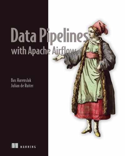
The most important of these parameters is called the execution_date, which represents the date and time for which our DAG is being executed. Contrary to what the name of the parameter suggests, the execution_date is not a date but a timestamp, which reflects the start time of the schedule interval for which the DAG is being executed. The end time of the schedule interval is indicated by another parameter called the next_execution_date. Together these dates define the entire length of a task’s schedule interval (figure 3.4).
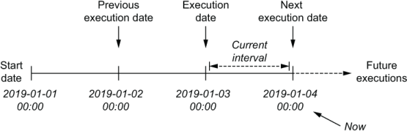
Figure 3.4 Execution dates in Airflow
Airflow also provides a previous_execution_date parameter, which describes the start of the previous schedule interval. Although we won’t be using this parameter here, it can be useful for performing analyses that contrast data from the current time interval with results from the previous interval.
In Airflow, we can use these execution dates by referencing them in our operators. For example, in the BashOperator, we can use Airflow’s templating functionality to include the execution dates dynamically in our Bash command. Templating is covered in detail in chapter 4.
Listing 3.6 Using templating for specifying dates (dags/06_templated_query.py)
fetch_events = BashOperator(
    task_id="fetch_events",
    bash_command=(
         "mkdir -p /data && "
         "curl -o /data/events.json "
         "http://localhost:5000/events?"
         "start_date={{execution_date.strftime('%Y-%m-%d')}}"        ❶
         "&end_date={{next_execution_date.strftime('%Y-%m-%d')}}"    ❷
    ),
    dag=dag,
)
❶ Formatted execution_date inserted with Jinja templating
❷ next_execution_date holds the execution date of the next interval.
In this example, the syntax {{variable_name}} is an example of using Airflow’s Jinja-based (http://jinja.pocoo.org) templating syntax for referencing one of Airflow’s specific parameters. Here, we use this syntax to reference the execution dates and format them to the expected string format using the datetime strftime method (as both execution dates are datetime objects).
Because the execution_date parameters are often used in this fashion to reference dates as formatted strings, Airflow also provides several shorthand parameters for common date formats. For example, the ds and ds_nodash parameters are different representations of the execution_date, formatted as YYYY-MM-DD and YYYYMMDD, respectively. Similarly, next_ds, next_ds_nodash, prev_ds, and prev_ds_nodash provide shorthand notations for the next and previous execution dates, respectively.2
Using these shorthand notations, we can also write our incremental fetch command as follows.
Listing 3.7 Using template shorthand (dags/07_templated_query_ds.py)
fetch_events = BashOperator(
   task_id="fetch_events",
   bash_command=(
     "mkdir -p /data && "
     "curl -o /data/events.json "
      "http://localhost:5000/events?"
      "start_date={{ds}}&"              ❶
      "end_date={{next_ds}}"            ❷
   ),
   dag=dag,
)
❶ ds provides YYYY-MM-DD formatted execution_date.
❷ next_ds provides the same for next_execution_date.
This shorter version is quite a bit easier to read. However, for more complicated date (or datetime) formats, you will likely still need to use the more flexible strftime method.
3.3.3 Partitioning your data
Although our new fetch_events task now fetches events incrementally for each new schedule interval, the astute reader may have noticed that each new task is simply overwriting the result of the previous day, meaning that we are effectively not building any history.
One way to solve this problem is to simply append new events to the events.json file, which would allow us to build our history in a single JSON file. However, a drawback of this approach is that it requires any downstream processing jobs to load the entire data set, even if we are only interested in calculating statistics for a given day. Additionally, it also makes this file a single point of failure, by which we may risk losing our entire data set should this file become lost or corrupted.
An alternative approach is to divide our data set into daily batches by writing the output of the task to a file bearing the name of the corresponding execution date.
Listing 3.8 Writing event data to separate files per date (dags/08_templated_path.py)
fetch_events = BashOperator(
    task_id="fetch_events",
    bash_command=(
        "mkdir -p /data/events && "
        "curl -o /data/events/{{ds}}.json "      ❶
        "http://localhost:5000/events?"
        "start_date={{ds}}&"
        "end_date={{next_ds}}",
    dag=dag,
)
❶ Response written to templated filename
This would result in any data being downloaded for an execution date of 2019-01-01 being written to the file /data/events/2019-01-01.json.
This practice of dividing a data set into smaller, more manageable pieces is a common strategy in data storage and processing systems and is commonly referred to as partitioning, with the smaller pieces of a data set the partitions. The advantage of partitioning our data set by execution date becomes evident when we consider the second task in our DAG (calculate_stats), in which we calculate statistics for each day’s worth of user events. In our previous implementation, we were loading the entire data set and calculating statistics for our entire event history, every day.
Listing 3.9 Previous implementation for event statistics (dags/01_scheduled.py)
def _calculate_stats(input_path, output_path):
    """Calculates event statistics."""
    Path(output_path).parent.mkdir(exist_ok=True)
    events = pd.read_json(input_path)
    stats = events.groupby(["date", "user"]).size().reset_index()
    stats.to_csv(output_path, index=False)


calculate_stats = PythonOperator(
    task_id="calculate_stats",
    python_callable=_calculate_stats,
    op_kwargs={
        "input_path": "/data/events.json",
        "output_path": "/data/stats.csv",
    },
    dag=dag,
)
However, using our partitioned data set, we can calculate these statistics more efficiently for each separate partition by changing the input and output paths of this task to point to the partitioned event data and a partitioned output file.
Listing 3.10 Calculating statistics per execution interval (dags/08_templated_path.py)
def _calculate_stats(**context):                             ❶
   """Calculates event statistics."""
   input_path = context["templates_dict"]["input_path"]      ❷
   output_path = context["templates_dict"]["output_path"]

   Path(output_path).parent.mkdir(exist_ok=True)

   events = pd.read_json(input_path)
   stats = events.groupby(["date", "user"]).size().reset_index()
   stats.to_csv(output_path, index=False)


calculate_stats = PythonOperator(
   task_id="calculate_stats",
   python_callable=_calculate_stats,
   templates_dict={
       "input_path": "/data/events/{{ds}}.json",             ❸
       "output_path": "/data/stats/{{ds}}.csv",
   },
   dag=dag,
)
❶ Receive all context variables in this dict.
❷ Retrieve the templated values from the templates_dict object.
❸ Pass the values that we want to be templated.
Although these changes may look somewhat complicated, they mostly involve boilerplate code for ensuring that our input and output paths are templated. To achieve this templating in the PythonOperator, we need to pass any arguments that should be templated using the operator’s templates_dict parameter. We then can retrieve the templated values inside our function from the context object that is passed to our _calculate_stats function by Airflow.3
If this all went a bit too quickly, don’t worry; we’ll dive into the task context in more detail in the next chapter. The important point to understand here is that these changes allow us to compute our statistics incrementally, by only processing a small subset of our data each day.
3.4 Understanding Airflow’s execution dates
Because execution dates are such an important part of Airflow, let’s take a minute to make sure we fully understand how these dates are defined.
3.4.1 Executing work in fixed-length intervals
As we’ve seen, we can control when Airflow runs a DAG with three parameters: a start date, a schedule interval, and an (optional) end date. To actually start scheduling our DAG, Airflow uses these three parameters to divide time into a series of schedule intervals, starting from the given start date and optionally ending at the end date (figure 3.5).
Figure 3.5 Time represented in terms of Airflow’s scheduling intervals. Assumes a daily interval with a start date of 2019-01-01.
In this interval-based representation of time, a DAG is executed for a given interval as soon as the time slot of that interval has passed. For example, the first interval in figure 3.5 would be executed as soon as possible after 2019-01-01 23:59:59, because by then the last time point in the interval has passed. Similarly, the DAG would execute for the second interval shortly after 2019-01-02 23:59:59, and so on, until we reach our optional end date.
An advantage of using this interval-based approach is that it is ideal for performing the type of incremental data processing we saw in the previous sections, as we know exactly for which interval of time a task is executing for—the start and end of the corresponding interval. This is in stark contrast to, for example, a time point–based scheduling system such as cron, where we only know the current time for which our task is being executed. This means that, for example in cron, we either have to calculate or guess where our previous execution left off by assuming that the task is executing for the previous day (figure 3.6).
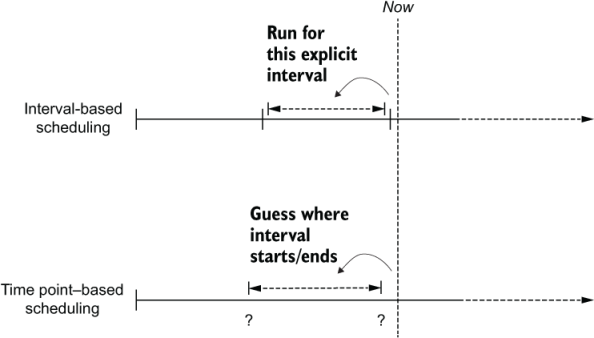
Figure 3.6 Incremental processing in interval-based scheduling windows (e.g., Airflow) versus windows derived from time point–based systems (e.g., cron). For incremental (data) processing, time is typically divided into discrete time intervals that are processed as soon as the corresponding interval has passed. Interval-based scheduling approaches (such as Airflow) explicitly schedule tasks to run for each interval while providing exact information to each task concerning the start and the end of the interval. In contrast, time point–based scheduling approaches only execute tasks at a given time, leaving it up to the task itself to determine for which incremental interval the task is executing.
Understanding that Airflow’s handling of time is built around schedule intervals also helps understand how execution dates are defined within Airflow. For example, say we have a DAG that follows a daily schedule interval, and then consider the corresponding interval that should process data for 2019-01-03. In Airflow, this interval will be run shortly after 2019-01-04 00:00:00, because at that point we know we will no longer be receiving any new data for 2019-01-03. Thinking back to our explanation of using execution dates in our tasks from the previous section, what do you think that the value of execution_date will be for this interval?
Many people expect that the execution date of this DAG run will be 2019-01-04, as this is the moment at which the DAG is actually run. However, if we look at the value of the execution_date variable when our tasks are executed, we will actually see an execution date of 2019-01-03. This is because Airflow defines the execution date of a DAG as the start of the corresponding interval. Conceptually, this makes sense if we consider that the execution date marks our schedule interval rather than the moment our DAG is actually executed. Unfortunately, the naming can be a bit confusing.
With Airflow execution dates being defined as the start of the corresponding schedule intervals, they can be used to derive the start and end of a specific interval (figure 3.7). For example, when executing a task, the start and end of the corresponding interval are defined by the execution_date (the start of the interval) and the next_execution date (the start of the next interval) parameters. Similarly, the previous schedule interval can be derived using the previous_execution_date and execution_date parameters.
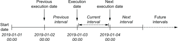
Figure 3.7 Execution dates in the context of schedule intervals. In Airflow, the execution date of a DAG is defined as the start time of the corresponding schedule interval rather than the time at which the DAG is executed (which is typically the end of the interval). As such, the value of execution_date points to the start of the current interval, while the previous_execution_date and next_execution_date parameters point to the start of the previous and next schedule intervals, respectively. The current interval can be derived from a combination of the execution_date and the next_execution_date, which signifies the start of the next interval and thus the end of the current one.
However, one caveat to keep in mind when using the previous_execution_date and next_execution_date parameters in your tasks is that these are only defined for DAG runs following the schedule interval. As such, the values of these parameters will be undefined for any runs that are triggered manually using Airflow UI or CLI because Airflow cannot provide information about next or previous schedule intervals if you are not following a schedule interval.
3.5 Using backfilling to fill in past gaps
As Airflow allows us to define schedule intervals from an arbitrary start date, we can also define past intervals from a start date in the past. We can use this property to perform historical runs of our DAG for loading or analyzing past data sets—a process typically referred to as backfilling.
3.5.1 Executing work back in time
By default, Airflow will schedule and run any past schedule intervals that have not been run. As such, specifying a past start date and activating the corresponding DAG will result in all intervals that have passed before the current time being executed. This behavior is controlled by the DAG catchup parameter and can be disabled by setting catchup to false.
Listing 3.11 Disabling catchup to avoid running past runs (dags/09_no_catchup.py)
dag = DAG(
   dag_id="09_no_catchup",
   schedule_interval="@daily",
   start_date=dt.datetime(year=2019, month=1, day=1),
   end_date=dt.datetime(year=2019, month=1, day=5),
   catchup=False,
)
With this setting, the DAG will only be run for the most recent schedule interval rather than executing all open past intervals (figure 3.8). The default value for catchup can be controlled from the Airflow configuration file by setting a value for the catchup_by_default configuration setting.

Figure 3.8 Backfilling in Airflow. By default, Airflow will run tasks for all past intervals up to the current time. This behavior can be disabled by setting the catchup parameter of a DAG to false, in which case Airflow will only start executing tasks from the current interval.
Although backfilling is a powerful concept, it is limited by the availability of data in source systems. For example, in our example use case we can load past events from our API by specifying a start date up to 30 days in the past. However, as the API only provides up to 30 days of history, we cannot use backfilling to load data from earlier days.
Backfilling can also be used to reprocess data after we have made changes in our code. For example, say we make a change to our calc_statistics function to add a new statistic. Using backfilling, we can clear past runs of our calc_statistics task to reanalyze our historical data using the new code. Note that in this case we aren’t limited by the 30-day limit of our data source, as we have already loaded these earlier data partitions as part of our past runs.
3.6 Best practices for designing tasks
Although Airflow does much of the heavy lifting when it comes to backfilling and rerunning tasks, we need to ensure our tasks fulfill certain key properties for proper results. In this section, we dive into two of the most important properties of proper Airflow tasks: atomicity and idempotency.
3.6.1 Atomicity
The term atomicity is frequently used in database systems, where an atomic transaction is considered an indivisible and irreducible series of database operations such that either all occur or nothing occurs. Similarly, in Airflow, tasks should be defined so that they either succeed and produce some proper result or fail in a manner that does not affect the state of the system (figure 3.9).

Figure 3.9 Atomicity ensures either everything or nothing completes. No half work is produced, and as a result, incorrect results are avoided down the line.
As an example, consider a simple extension to our user event DAG, in which we would like to add some functionality that sends an email of our top 10 users at the end of each run. One simple way to add this is to extend our previous function with an additional call to some function that sends an email containing our statistics.
Listing 3.12 Two jobs in one task, to break atomicity (dags/10_non_atomic_send.py)
def _calculate_stats(**context):
    """Calculates event statistics."""
    input_path = context["templates_dict"]["input_path"]
    output_path = context["templates_dict"]["output_path"]

    events = pd.read_json(input_path)
    stats = events.groupby(["date", "user"]).size().reset_index()
    stats.to_csv(output_path, index=False)

    email_stats(stats, email="[email protected]")      ❶
❶ Sending an email after writing to CSV creates two pieces of work in a single function, which breaks the atomicity of the task.
Unfortunately, a drawback of this approach is that the task is no longer atomic. Can you see why? If not, consider what happens if our _send_stats function fails (which is bound to happen if our email server is a bit flaky). In this case, we will already have written our statistics to the output file at output_path, making it seem as if our task succeeded even though it ended in failure.
To implement this functionality in an atomic fashion, we could simply split the email functionality into a separate task.
Listing 3.13 Splitting into multiple tasks to improve atomicity (dags/11_atomic_send.py)
def _send_stats(email, **context):
    stats = pd.read_csv(context["templates_dict"]["stats_path"])
    email_stats(stats, email=email)                                ❶


send_stats = PythonOperator(
    task_id="send_stats",
    python_callable=_send_stats,
    op_kwargs={"email": "[email protected]"},
    templates_dict={"stats_path": "/data/stats/{{ds}}.csv"},
    dag=dag,
)

calculate_stats >> send_stats
❶ Split off the email_stats statement into a separate task for atomicity.
This way, failing to send an email no longer affects the result of the calculate_stats task, but only fails send_stats, thus making both tasks atomic.
From this example, you might think that separating all operations into individual tasks is sufficient to make all our tasks atomic. However, this is not necessarily true. To understand why, think about if our event API had required us to log in before querying for events. This would generally require an extra API call to fetch some authentication token, after which we can start retrieving our events.
Following our previous reasoning of one operation = one task, we would have to split these operations into two separate tasks. However, doing so would create a strong dependency between them, as the second task (fetching the events) will fail without running the first shortly before. This strong dependency between means we are likely better off keeping both operations within a single task, allowing the task to form a single, coherent unit of work.
Most Airflow operators are already designed to be atomic, which is why many operators include options for performing tightly coupled operations such as authentication internally. However, more flexible operators such as the Python and Bash operators may require you to think carefully about your operations to make sure your tasks remain atomic.
3.6.2 Idempotency
Another important property to consider when writing Airflow tasks is idempotency. Tasks are said to be idempotent if calling the same task multiple times with the same inputs has no additional effect. This means that rerunning a task without changing the inputs should not change the overall output.
For example, consider our last implementation of the fetch_events task, which fetches the results for a single day and writes this to our partitioned data set.
Listing 3.14 Existing implementation for fetching events (dags/08_templated_paths.py)
fetch_events = BashOperator(
    task_id="fetch_events",
    bash_command=(
        "mkdir -p /data/events && "
        "curl -o /data/events/{{ds}}.json "       ❶
        "http://localhost:5000/events?"
        "start_date={{ds}}&"
        "end_date={{next_ds}}"
    ),
    dag=dag,
)
❶ Partitioning by setting templated filename
Rerunning this task for a given date would result in the task fetching the same set of events as its previous execution (assuming the date is within our 30-day window), and overwriting the existing JSON file in the /data/events folder, producing the same result. As such, this implementation of the fetch events task is clearly idempotent.
To show an example of a non-idempotent task, consider using a single JSON file (/data/events.json) and simply appending events to this file. In this case, rerunning a task would result in the events simply being appended to the existing data set, thus duplicating the day’s events (figure 3.10). As such, this implementation is not idempotent, as additional executions of the task change the overall result.

Figure 3.10 An idempotent task produces the same result, no matter how many times you run it. Idempotency ensures consistency and the ability to deal with failure.
In general, tasks that write data can be made idempotent by checking for existing results or making sure that previous results are overwritten by the task. In time-partitioned data sets, this is relatively straightforward, as we can simply overwrite the corresponding partition. Similarly, for database systems, we can use upsert operations to insert data, which allows us to overwrite existing rows that were written by previous task executions. However, in more general applications, you should carefully consider all side effects of your task and make sure they are performed in an idempotent fashion.
Summary
-
DAGs can run at regular intervals by setting the schedule interval.
-
The work for an interval is started at the end of the interval.
-
The schedule interval can be configured with cron and timedelta expressions.
-
Data can be processed incrementally by dynamically setting variables with templating.
-
The execution date refers to the start datetime of the interval, not to the actual time of execution.
-
Idempotency ensures tasks can be rerun while producing the same output results.
1.https://crontab.guru translates cron expressions to human-readable language.
2.See https://airflow.readthedocs.io/en/stable/macros-ref.html for an overview of all available shorthand options.
3.For Airflow 1.10.x, you’ll need to pass the extra argument provide_context=True to the PythonOperator; otherwise, the _calculate_stats function won’t receive the context values.