- Writing clean, understandable DAGs using style conventions
- Using consistent approaches for managing credentials and configuration options
- Generating repeated DAGs and tasks using factory functions
- Designing reproducible tasks by enforcing idempotency and determinism constraints
- Handling data efficiently by limiting the amount of data processed in your DAG
- Using efficient approaches for handling/storing (intermediate) data sets
- Managing managing concurrency using resource pools
In previous chapters, we have described most of the basic elements that go into building and designing data processes using Airflow DAGs. In this chapter, we dive a bit deeper into some best practices that can help you write well-architected DAGs that are both easy to understand and efficient in terms of how they handle your data and resources.
11.1 Writing clean DAGs
Writing DAGs can easily become a messy business. For example, DAG code can quickly become overly complicated or difficult to read—especially if DAGs are written by team members with very different styles of programming. In this section, we touch on some tips to help you structure and style your DAG code, hopefully providing some (often needed) clarity for your intricate data processes.
11.1.1 Use style conventions
As in all programming exercises, one of the first steps to writing clean and consistent DAGs is to adopt a common, clean programming style and apply this style consistently across all your DAGs. Although a thorough exploration of clean coding practices is well outside the scope of this book, we can provide several tips as starting points.
The easiest way to make your code cleaner and easier to understand is to use a commonly used style when writing your code. There are multiple style guides available in the community, including the widely known PEP8 style guide (https://www.python.org/dev/peps/pep-0008/) and guides from companies such as Google (https://google.github.io/styleguide/pyguide.html). These generally include recommendations for indentation, maximum line lengths, naming styles for variables/classes/functions, and so on. By following these guides, other programmers will be better able to read your code.
Listing 11.1 Examples of non-PEP8-compliant code
spam( ham[ 1 ], { eggs: 2 } )

i=i+1
submitted +=1

my_list = [
    1, 2, 3,
    4, 5, 6,
    ]
Listing 11.2 Making the examples in listing 11.1 PEP-8 compliant
spam(ham[1], {eggs: 2})   ❶

i = i + 1                 ❷
submitted += 1            ❷

my_list = [               ❸
    1, 2, 3,
    4, 5, 6,
]
❷ Consistent whitespace around operators
❸ More readable indenting around list brackets
Using static checkers to check code quality
The Python community has also produced a plethora of software tools that can be used to check whether your code follows proper coding conventions and/or styles. Two popular tools are Pylint and Flake8, which both function as static code checkers, meaning that you can run them over your code to get a report of how well (or not) your code adheres to their envisioned standards.
For example, to run Flake8 over your code, you can install it using pip and run it by pointing it at your codebase.
Listing 11.3 Installing and running Flake8
python -m pip install flake8
python -m flake8 dags/*.py
This command will run Flake8 on all of the Python files in the DAGs folder, giving you a report on the perceived code quality of these DAG files. The report will typically look something like this.
Listing 11.4 Example output from Flake8
$ python -m flake8 chapter08/dags/
chapter08/dags/04_sensor.py:2:1: F401
 ➥ 'airflow.operators.python.PythonOperator' imported but unused
chapter08/dags/03_operator.py:2:1: F401
 ➥ 'airflow.operators.python.PythonOperator' imported but unused
Both Flake8 and Pylint are used widely within the community, although Pylint is generally considered to have a more extensive set of checks in its default configuration.1 Of course, both tools can be configured to enable/disable certain checks, depending on your preferences, and can be combined to provide comprehensive feedback. For more details, we refer you to the respective websites of both tools.
Using code formatters to enforce common formatting
Although static checkers give you feedback on the quality of your code, tools such as Pylint or Flake8 do not impose overly strict requirements on how you format your code (e.g., when to start a new line, how to indent your function headers, etc.). As such, Python code written by different people can still follow very different formatting styles, depending on the preferences of the author.
One approach to reducing the heterogeneity of code formatting within teams is to use a code formatter to surrender control (and worry) to the formatting tool, which will ensure that your code is reformatted according to its guidelines. As such, applying a formatter consistently across your project will ensure all code follows one consistent formatting style: the style implemented by the formatter.
Two commonly used code Python formatters are YAPF (https://github.com/google/ yapf) and Black (https://github.com/psf/black). Both tools adopt a similar style of taking your Python code and reformatting it to their styles, with slight differences in the styles enforced by both. As such, the choice between Black and YAPF may depend on personal preference, although Black has gained much popularity within the Python community over the past few years.
To show a small example, consider the following (contrived) example of an ugly function.
Listing 11.5 Code example before Black formatting
def my_function(
    arg1, arg2,
    arg3):
    """Function to demonstrate black."""
    str_a = 'abc'
    str_b = "def"
    return str_a +
        str_b
Applying Black to this function will give you the following (cleaner) result.
Listing 11.6 The same code example after Black formatting
def my_function(arg1, arg2, arg3):         ❶
    """Function to demonstrate black."""
    str_a = "abc"                          ❷
    str_b = "def"                          ❷
    return str_a + str_b                   ❸
❶ More consistent indenting for arguments
❷ Consistent use of double quotes
❸ Unnecessary line break removed
To run Black yourself, install it using pip and apply it to your Python files using the following.
Listing 11.7 Installing and running black
python -m pip install black
python -m black dags/
This should give you something like the following output, indicating whether Black reformatted any Python files for you.
Listing 11.8 Example output from black
reformatted dags/example_dag.py
All done! ✨ ? ✨
1 file reformatted.
Note that you can also perform a dry run of Black using the --check flag, which will cause Black to indicate only whether it would reformat any files rather than doing any actual reformatting.
Many editors (such as Visual Studio Code, Pycharm) support integration with these tools, allowing you to reformat your code from within your editor. For details on how to configure this type of integration, see the documentation of the respective editor.
Airflow-specific style conventions
It’s also a good idea to agree on style conventions for your Airflow code, particularly in cases where Airflow provides multiple ways to achieve the same results. For example, Airflow provides two different styles for defining DAGs.
Listing 11.9 Two styles for defining DAGs
with DAG(...) as dag:                  ❶
    task1 = PythonOperator(...)
    task2 = PythonOperator(...)

dag = DAG(...)                         ❷
task1 = PythonOperator(..., dag=dag)
task2 = PythonOperator(..., dag=dag)
In principle, both these DAG definitions do the same thing, meaning that there is no real reason to choose one over the other, outside of style preferences. However, within your team it may be a good idea to choose one of the two styles and follow them throughout your codebase, keeping things more consistent and understandable.
This consistency is even more important when defining dependencies between tasks, as Airflow provides several different ways for defining the same task dependency.
Listing 11.10 Different styles for defining task dependencies
task1 >> task2
task1 << task2
[task1] >> task2
task1.set_downstream(task2)
task2.set_upstream(task1)
Although these different definitions have their own merits, combining different styles of dependency definitions within a single DAG can be confusing.
Listing 11.11 Mixing different task dependency notations
task1 >> task2
task2 << task3
task5.set_upstream(task3)
task3.set_downstream(task4)
As such, your code will generally be more readable if you stick to a single style for defining dependencies across tasks.
Listing 11.12 Using a consistent style for defining task dependencies
task1 >> task2 >> task3 >> [task4, task5]
As before, we don’t necessarily have a clear preference for any given style; just make sure that you pick one that you (and your team) like and apply it consistently.
11.1.2 Manage credentials centrally
In DAGs that interact with many different systems, you may find yourself juggling with many different types of credentials—databases, compute clusters, cloud storage, and so on. As we’ve seen in previous chapters, Airflow allows you to maintain these credentials in its connection store, which ensures your credentials are maintained securely2 in a central location.
Although the connection store is the easiest place to store credentials for built-in operators, it can be tempting to store secrets for your custom PythonOperator functions (and other functions) in less secure places for ease of accessibility. For example, we have seen quite a few DAG implementations with security keys hardcoded into the DAG itself or in external configuration files.
Fortunately, it is relatively easy to use the Airflow connections store to maintain credentials for your custom code too, by retrieving the connection details from the store in your custom code and using the obtained credentials to do your work.
Listing 11.13 Fetching credentials from the Airflow metastore
from airflow.hooks.base_hook import BaseHook

def _fetch_data(conn_id, **context)
    credentials = BaseHook.get_connection(conn_id)      ❶
    ...

fetch_data = PythonOperator(
    task_id="fetch_data",
    op_kwargs={"conn_id": "my_conn_id"},
    dag=dag
)
❶ Fetching credentials using the given ID
An advantage of this approach is that it uses the same method of storing credentials as all other Airflow operators, meaning that credentials are managed in one single place. As a consequence, you only have to worry about securing and maintaining credentials in this central database.
Of course, depending on your deployment you may want to maintain your secrets in other external systems (e.g., Kubernetes secrets, cloud secret stores) before passing them into Airflow. In this case, it is still a good idea to make sure these credentials are passed into Airflow (using environment variables, for example) and that your code accesses them using the Airflow connection store.
11.1.3 Specify configuration details consistently
You may have other parameters you need to pass in as configuration to your DAG, such as file paths, table names, and so on. Because they are written in Python, Airflow DAGs provide you with many different options for configuration options, including global variables (within the DAG), configuration files (e.g., YAML, INI, JSON), environment variables, Python-based configuration modules, and so on. Airflow also allows you to store configurations in the metastore using Variables (https://airflow.apache.org/docs/stable/concepts.html#variables).
For example, to load some configuration options from a YAML file3 you might use something like the following.
Listing 11.14 Loading configuration options from a YAML file
import yaml

with open("config.yaml") as config_file:
    config = yaml.load(config_file)         ❶
...
fetch_data = PythonOperator(
    task_id="fetch_data",
    op_kwargs={
        "input_path": config["input_path"],
        "output_path": config["output_path"],
    },
    ...
)
❶ Read config file using PyYAML.
Listing 11.15 Example YAML configuration file
input_path: /data
output_path: /output
Similarly, you could also load the config using Airflow Variables, which is essentially an Airflow feature for storing (global) variables in the metastore.4
Listing 11.16 Storing configuration options in Airflow Variables
from airflow.models import Variable

input_path = Variable.get("dag1_input_path")        ❶
output_path = Variable.get("dag1_output_path")

fetch_data = PythonOperator(
    task_id="fetch_data",
    op_kwargs={
        "input_path": input_path,
        "output_path": output_path,
    },
    ...
)
❶ Fetching global variables using Airflow’s Variable mechanism
Note that fetching Variables in the global scope like this can be a bad idea, as this means Airflow will refetch them from the database every time the scheduler reads your DAG definition.
In general, we don’t have any real preference for how you store your config, as long as you are consistent about it. For example, if you store your configuration for one DAG as a YAML file, it makes sense to follow the same convention for other DAGs as well.
For configuration that is shared across DAGs, it is highly recommended to specify the configuration values in a single location (e.g., a shared YAML file), following the DRY (don’t repeat yourself) principle. This way, you will be less likely to run into issues where you change a configuration parameter in one place and forget to change it in another.
Finally, it is good to realize that configuration options can be loaded in different contexts depending on where they are referenced within your DAG. For example, if you load a config file in the main part of your DAG, as follows.
Listing 11.17 Loading configuration options in the DAG definition (inefficient)
import yaml

with open("config.yaml") as config_file:
    config = yaml.load(config_file)         ❶

fetch_data = PythonOperator(...)
❶ In the global scope, this config will be loaded on the scheduler.
The config.yaml file is loaded from the local file system of the machine(s) running the Airflow webserver and/or scheduler. This means that both these machines should have access to the config file path. In contrast, you can also load the config file as part of a (Python) task.
Listing 11.18 Loading configuration options within a task (more efficient)
import yaml

def _fetch_data(config_path, **context):
    with open(config_path) as config_file:
        config = yaml.load(config_file)        ❶
    ...

fetch_data = PythonOperator(
    op_kwargs={"config_path": "config.yaml"},
    ...
)
❶ In task scope, this config will be loaded on the worker.
In this case, the config file won’t be loaded until your function is executed by an Airflow worker, meaning that the config is loaded in the context of the Airflow worker. Depending on how you set up your Airflow deployment, this may be an entirely different environment (with access to different file systems, etc.), leading to erroneous results or failures. Similar situations may occur with other configuration approaches as well.
You can avoid these types of situations by choosing one configuration approach that works well and sticking with it across DAGs. Also, be mindful of where different parts of your DAG are executed when loading configuration options and preferably use approaches that are accessible to all Airflow components (e.g., nonlocal file systems, etc.).
11.1.4 Avoid doing any computation in your DAG definition
Airflow DAGs are written in Python, which gives you a great deal of flexibility when writing them. However, a drawback of this approach is that Airflow needs to execute your Python DAG file to derive the corresponding DAG. Moreover, to pick up any changes you may have made to your DAG, Airflow has to reread the file at regular intervals and sync any changes to its internal state.
As you can imagine, this repeated parsing of your DAG files can lead to problems if any of them take a long time to load. This can happen, for example, if you do any long-running or heavy computations when defining your DAG.
Listing 11.19 Performing computations in the DAG definition (inefficient)
...
task1 = PythonOperator(...)
my_value = do_some_long_computation()           ❶
task2 = PythonOperator(op_kwargs={"my_value": my_value})
...
❶ This long computation will be computed every time the DAG is parsed.
This kind of implementation will cause Airflow to execute do_some_long_computation every time the DAG file is loaded, blocking the entire DAG parsing process until the computation has finished.
One way to avoid this issue to postpone the computation to the execution of the task that requires the computed value.
Listing 11.20 Performing computations within tasks (more efficient)
def _my_not_so_efficient_task(value, ...):
    ...

PythonOperator(
    task_id="my_not_so_efficient_task",
    ...
    op_kwargs={
        "value": calc_expensive_value()         ❶
    }
)

def _my_more_efficient_task(...):
    value = calc_expensive_value()              ❷
    ...

PythonOperator(
    task_id="my_more_efficient_task",
    python_callable=_my_more_efficient_task,    ❷
    ...
)
❶ Here, the value will be computed every time the DAG is parsed.
❷ By moving the computation into the task, the value will only be calculated when the task is executed.
Another approach would be to write our own hook/operator, which only fetches credentials when needed for execution, but this may require a bit more work.
Something similar may occur in more subtle cases, in which a configuration is loaded from an external data source or file system in your main DAG file. For example, we may want to load credentials from the Airflow metastore and share them across a few tasks by doing something like this.
Listing 11.21 Fetching credentials from the metastore in the DAG definition (inefficient)
from airflow.hooks.base_hook import BaseHook

api_config = BaseHook.get_connection("my_api_conn")      ❶
api_key = api_config.login
api_secret = api_config.password

task1 = PythonOperator(
    op_kwargs={"api_key": api_key, "api_secret": api_secret},
    ...
)
...
❶ This call will hit the database every time the DAG is parsed.
However, a drawback of this approach is that it fetches credentials from the database every time our DAG is parsed instead of only when the DAG is executed. As such, we will see repeated queries every 30 seconds or so (depending on the Airflow config) against our database, simply for retrieving these credentials.
These types of performance issues can generally be avoided by postponing the fetching of credentials to the execution of the task function.
Listing 11.22 Fetching credentials within a task (more efficient)
from airflow.hooks.base_hook import BaseHook

def _task1(conn_id, **context):
    api_config = BaseHook.get_connection(conn_id)      ❶
    api_key = api_config.login
    api_secret = api_config.password
    ...

task1 = PythonOperator(op_kwargs={"conn_id": "my_api_conn"})
❶ This call will only hit the database when the task is executed.
This way, credentials are only fetched when the task is actually executed, making our DAG much more efficient. This type of computation creep, in which you accidentally include computations in your DAG definitions, can be subtle and requires some vigilance to avoid. Also, some cases may be worse than others: you may not mind repeatedly loading a configuration file from a local file system, but repeatedly loading from a cloud storage or database may be less preferable.
11.1.5 Use factories to generate common patterns
In some cases, you may find yourself writing variations of the same DAG over and over again. This often occurs in situations where you are ingesting data from related data sources, with only small variations in source paths and any transformations applied to the data. Similarly, you may have common data processes within your company that require many of the same steps/transformations and as a result are repeated across many different DAGs.
One effective way to speed up the process of generating these common DAG structures is to write a factory function. The idea behind such a function is that it takes any required configuration for the respective steps and generates the corresponding DAG or set of tasks (thus producing it, like a factory). For example, if we have a common process that involves fetching some data from an external API and preprocessing this data using a given script, we could write a factory function that looks a bit like this.
Listing 11.23 Generating sets of tasks with a factory function (dags/01_task_factory.py)
def generate_tasks(dataset_name, raw_dir, processed_dir,
                   preprocess_script, output_dir, dag):                    ❶
    raw_path = os.path.join(raw_dir, dataset_name, "{ds_nodash}.json")     ❷
    processed_path = os.path.join(
        processed_dir, dataset_name, "{ds_nodash}.json"
    )
    output_path = os.path.join(output_dir, dataset_name, "{ds_nodash}.json")
   fetch_task = BashOperator(                                              ❸
       task_id=f"fetch_{dataset_name}",
       bash_command=f"echo 'curl http://example.com/{dataset_name}.json
         ➥ > {raw_path}.json'",
       dag=dag,
   )

   preprocess_task = BashOperator(
       task_id=f"preprocess_{dataset_name}",
       bash_command=f"echo '{preprocess_script} {raw_path}
         ➥ {processed_path}'",
       dag=dag,
   )

   export_task = BashOperator(
       task_id=f"export_{dataset_name}",
       bash_command=f"echo 'cp {processed_path} {output_path}'",
       dag=dag,
   )

fetch_task >> preprocess_task >> export_task                               ❹

return fetch_task, export_task                                             ❺
❶ Parameters that configure the tasks that will be created by the factory function
❷ File paths used by the different tasks
❸ Creating the individual tasks
❺ Return the first and last tasks in the chain so that we can connect them to other tasks in the larger graph (if needed).
We could then use this factory function to ingest multiple data sets like this.
Listing 11.24 Applying the task factory function (dags/01_task_factory.py)
import airflow.utils.dates
from airflow import DAG

with DAG(
    dag_id="01_task_factory",
    start_date=airflow.utils.dates.days_ago(5),
    schedule_interval="@daily",
) as dag:
    for dataset in ["sales", "customers"]:
        generate_tasks(                                     ❶
            dataset_name=dataset,
            raw_dir="/data/raw",
            processed_dir="/data/processed",
            output_dir="/data/output",
            preprocess_script=f"preprocess_{dataset}.py",
            dag=dag,                                        ❷
        )
❶ Creating sets of tasks with different configuration values
❷ Passing the DAG instance to connect the tasks to the DAG
This should give us a DAG similar to the one in figure 11.1. Of course, for independent data sets, it would probably not make sense to ingest the two in a single DAG. You can, however, easily split the tasks across multiple DAGs by calling the generate_tasks factory method from different DAG files.
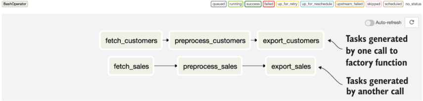
Figure 11.1 Generating repeated patterns of tasks using factory methods. This example DAG contains multiple sets of almost identical tasks, which were generated from a configuration object using a task factory method.
You can also write factory methods for generating entire DAGs, as shown in listing 11.25.
Listing 11.25 Generating DAGs with a factory function (dags/02_dag_factory.py)
def generate_dag(dataset_name, raw_dir, processed_dir, preprocess_script):
    with DAG(
        dag_id=f"02_dag_factory_{dataset_name}",
        start_date=airflow.utils.dates.days_ago(5),
        schedule_interval="@daily",
    ) as dag:                            ❶
        raw_file_path = ...
        processed_file_path = ...

        fetch_task = BashOperator(...)
        preprocess_task = BashOperator(...)

        fetch_task >> preprocess_task

    return dag
❶ Generating the DAG instance within the factory function
This would allow you to generate a DAG using the following, minimalistic DAG file.
Listing 11.26 Applying the DAG factory function
...

dag = generate_dag(           ❶
    dataset_name="sales",
        raw_dir="/data/raw",
        processed_dir="/data/processed",
        preprocess_script="preprocess_sales.py",
)
❶ Creating the DAG using the factory function
You can also use this kind of approach to generate multiple DAGs using a DAG file.
Listing 11.27 Generating multiple DAGs with a factory function (dags/02_dag_factory.py)
...

for dataset in ["sales", "customers"]:
    globals()[f"02_dag_factory_{dataset}"] = generate_dag(      ❶
        dataset_name=dataset,
        raw_dir="/data/raw",
        processed_dir="/data/processed",
        preprocess_script=f"preprocess_{dataset}.py",
    )
❶ Generating multiple DAGs with different configurations. Note we have to assign each DAG a unique name in the global namespace (using the globals trick) to make sure they don’t overwrite each other.
This loop effectively generates multiple DAG objects in the global scope of your DAG file, which Airflow picks up as separate DAGs (figure 11.2). Note that the objects need to have different variable names to prevent them from overwriting each other; otherwise, Airflow will only see a single DAG instance (the last one generated by the loop).

Figure 11.2 Multiple DAGs generated from a single file using a DAG factory function. (Screenshot taken from the Airflow UI, showing multiple DAGs that were generated from a single DAG file using a DAG factory function.)
We recommend some caution when generating multiple DAGs from a single DAG file, as it can be confusing if you’re not expecting it. (The more general pattern is to have one file for each DAG.) As such, this pattern is best used sparingly when it provides significant benefits.
Task or DAG factory methods can be particularly powerful when combined with configuration files or other forms of external configuration. This allows you to, for example, build a factory function that takes a YAML file as input and generates a DAG based on the configuration defined in that file. This way, you can configure repetitive ETL processes using a bunch of relatively simple configuration files, which can also be edited by users who have little knowledge of Airflow.
11.1.6 Group related tasks using task groups
Complex Airflow DAGs, particularly those generated using factory methods, can often become difficult to understand due to complex DAG structures or the sheer number of tasks involved. To help organize these complex structures, Airflow 2 has a new feature called task groups. Task groups effectively allow you to (visually) group sets of tasks into smaller groups, making your DAG structure easier to oversee and comprehend.
You can create task groups using the TaskGroup context manager. For example, taking our previous task factory example, we can group the tasks generated for each data set as follows.
Listing 11.28 Using TaskGroups to visually group tasks (dags/03_task_groups.py)
...
for dataset in ["sales", "customers"]:
    with TaskGroup(dataset, tooltip=f"Tasks for processing {dataset}"):
        generate_tasks(
            dataset_name=dataset,
            raw_dir="/data/raw",
            processed_dir="/data/processed",
            output_dir="/data/output",
            preprocess_script=f"preprocess_{dataset}.py",
            dag=dag,
    )
This effectively groups the set of tasks generated for the sales and customers data sets into two task groups, one for each data set. As a result, the grouped tasks are shown as a single condensed task group in the web interface, which can be expanded by clicking on the respective group (figure 11.3).

Figure 11.3 Task groups can help organize DAGs by grouping related tasks. Initially, task groups are depicted as single nodes in the DAG, as shown for the customers task group in this figure. By clicking on a task group you can expand it and view the tasks within the group, as shown here for the sales task group. Note that task groups can be nested, meaning that you can have task groups within task groups.
Although this is a relatively simple example, the task group feature can be quite effective in reducing the amount of visual noise in more complex cases. For example, in our DAG for training machine learning models in chapter 5, we created a considerable number of tasks for fetching and cleaning weather and sales data from different systems. Task groups allow us to reduce the apparent complexity of this DAG by grouping the sales- and weather-related tasks into their respective task groups. This allows us to hide the complexity of the data set fetching tasks by default but still zoom in on the individual tasks when needed (figure 11.4).

Figure 11.4 Using task groups to organize the umbrella DAG from chapter 5. Here, grouping the tasks for fetching and cleaning the weather and sales data sets helps greatly simplify the complex task structures involved in these processes. (Code example is given in dags/04_task_groups_umbrella.py.)
11.1.7 Create new DAGs for big changes
Once you’ve started running a DAG, the scheduler database contains instances of the runs of that DAG. Big changes to the DAG, such as to the start date and/or schedule interval, may confuse the scheduler, as the changes no longer fit with previous DAG runs. Similarly, removing or renaming tasks will prevent you from accessing the history of those tasks from the UI, as they will no longer match the current state of the DAG and will therefore no longer be displayed.
The best way to avoid these issues is to create a new version of the DAG whenever you decide to make big changes to existing ones, as Airflow does not support versioned DAGs at this time. You can do this by creating a new versioned copy of the DAG (i.e., dag_v1, dag_v2) before making the desired changes. This way, you can avoid confusing the scheduler while also keeping historical information about the old version available. Support for versioned DAGs may be added in the future, as there is a strong desire in the community to do so.
11.2 Designing reproducible tasks
Aside from your DAG code, one of the biggest challenges in writing a good Airflow DAG is designing your tasks to be reproducible, meaning that you can easily rerun a task and expect the same result—even if the task is run at different points in time. In this section, we revisit some key ideas and offer some advice on ensuring your tasks fit into this paradigm.
11.2.1 Always require tasks to be idempotent
As briefly discussed in chapter 3, one of the key requirements for a good Airflow task is that the task is idempotent, meaning that rerunning the same task multiple times gives the same overall result (assuming the task itself has not changed).
Idempotency is an important characteristic because there are many situations in which you or Airflow may rerun a task. For example, you may want to rerun some DAG runs after changing some code, leading to the re-execution of a given task. In other cases, Airflow itself may rerun a failed task using its retry mechanism, even though the given task did manage to write some results before failing. In both cases, you want to avoid introducing multiple copies of the same data in your environment or running into other undesirable side effects.
Idempotency can typically be enforced by requiring that any output data is overwritten when a task is rerun, as this ensures any data written by a previous run is overwritten by the new result. Similarly, you should carefully consider any other side effects of a task (such as sending notifications, etc.) and determine whether these violate the idempotency of your task in any detrimental way.
11.2.2 Task results should be deterministic
Tasks can only be reproducible if they are deterministic. This means that a task should always return the same output for a given input. In contrast, nondeterministic tasks prevent us from building reproducible DAGs, as every run of the task may give us a different result, even for the same input data.
Nondeterministic behavior can be introduced in various ways:
-
Relying on the implicit ordering of your data or data structures inside the function (e.g., the implicit ordering of a Python dict or the order of rows in which a data set is returned from a database, without any specific ordering)
-
Using external state within a function, including random values, global variables, external data stored on disk (not passed as input to the function), and so on
-
Performing data processing in parallel (across multiple processes/threads), without doing any explicit ordering on the result
In general, issues with nondeterministic functions can be avoided by carefully thinking about sources of nondeterminism that may occur within your function. For example, you can avoid nondeterminism in the ordering of your data set by applying an explicit sort to it. Similarly, any issues with algorithms that include randomness can be avoided by setting the random seed before performing the corresponding operation.
11.2.3 Design tasks using functional paradigms
One approach that may help in creating your tasks is to design them according to the paradigm of functional programming. Functional programming is an approach to building computer programs that essentially treats computation as the application of mathematical functions while avoiding changing state and mutable data. Additionally, functions in functional programming languages are typically required to be pure, meaning that they may return a result but otherwise do not have any side effects.
One of the advantages of this approach is that the result of a pure function in a functional programming language should always be the same for a given input. As such, pure functions are generally both idempotent and deterministic—exactly what we are trying to achieve for our tasks in Airflow functions. Therefore, proponents of the functional paradigm have argued that similar approaches can be applied to data-processing applications, introducing the functional data engineering paradigm.
Functional data engineering approaches essentially aim to apply the same concepts from functional programming languages to data engineering tasks. This includes requiring tasks to not have any side effects and to always have the same result when applied to the same input data set. The main advantage of enforcing these constraints is that they go a long way toward achieving our ideals of idempotent and deterministic tasks, thus making our DAGs and tasks reproducible.
For more details, refer to this blog post by Maxime Beauchemin (one of the key people behind Airflow), which provides an excellent introduction to the concept of functional data engineering for data pipelines in Airflow: http://mng.bz/2eqm.
11.3 Handling data efficiently
DAGs that are meant to handle large amounts of data should be carefully designed to do so in the most efficient manner possible. In this section, we’ll discuss a couple of tips on how to handle large data volumes efficiently.
11.3.1 Limit the amount of data being processed
Although this may sound a bit trivial, the best way to efficiently handle data is to limit your processing to the minimal data required to obtain the desired result. After all, processing data that is going to be discarded anyway is a waste of both time and resources.
In practice, this means carefully thinking about your data sources and determining if they are all required. For the data sets that are needed, you can try to see if you can reduce the size of them by discarding rows/columns that aren’t used. Performing aggregations early on can also substantially increase performance, as the right aggregation can greatly reduce the size of an intermediate data set—thus decreasing the amount of work that needs to be done downstream.
To give an example, imagine a data process in which we are interested in calculating the monthly sales volumes of our products among a particular customer base (figure 11.5). In this example, we can calculate the aggregate sales by first joining the two data sets, followed by an aggregation and filtering step in which we aggregate our sales to the required granularity then filtered for the required customers. A drawback of this approach is that we are joining two potentially large data sets to get our result, which may take considerable time and resources.

Figure 11.5 Example of an inefficient data process compared to a more efficient one. (A) One way to calculate the aggregate sales per customer is to first fully join both data sets and then aggregate sales to the required granularity and filter for the customers of interest. Although this may give the desired result, it is not very efficient due to the potentially large size of the joined table. (B) A more efficient approach is to first filter/aggregate the sales and customer tables down to the minimum required granularity, allowing us to join the two smaller data sets.
A more efficient approach is to push the filtering/aggregation steps forward, allowing us to reduce the size of the customer and sales data sets before joining them. This potentially allows us to greatly reduce the size of the joined data set, making our computation much more efficient.
Although this example may be a bit abstract, we have encountered many similar cases where smart aggregation or the filtering of data sets (both in terms of rows and columns) greatly increased the performance of the involved data processes. As such, it may be beneficial to carefully look at your DAGs and see if they are processing more data than needed.
11.3.2 Incremental loading/processing
In many cases, you may not be able to reduce the size of your data set using clever aggregation or filtering. However, especially for time series data sets, you can often also limit the amount of processing you need to do in each run of your processing by using incremental data processing.
The main idea behind incremental processing (which we touched on in chapter 3) is to split your data into (time-based) partitions and process them individually in each of your DAG runs. This way, you limit the amount of data being processed in each run to the size of the corresponding partition, which is usually much smaller than the size of the entire data set. However, by adding each run’s results as increments to the output data set, you’ll still build up the entire data set over time (figure 11.6).
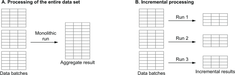
Figure 11.6 Illustration of monolithic processing (A), in which the entire data set is processed on every run, compared to incremental processing (B), in which the data set is analyzed in incremental batches as data comes in
An advantage of designing your process to be incremental is that any error in one of the runs won’t require you to redo your analysis for the entire data set; you can simply restart the run that failed. Of course, in some cases you may still have to do analyses on the entire data set. However, you can still benefit from incremental processing by performing filtering/aggregation steps in the incremental part of your process and doing the large-scale analysis on the reduced result.
11.3.3 Cache intermediate data
In most data-processing workflows, DAGs consist of multiple steps that each perform additional operations on data coming from preceding steps. An advantage of this approach (as described earlier in this chapter) is that it breaks our DAG down into clear, atomic steps, which are easy to rerun if we encounter any errors.
However, to be able to rerun any steps in such a DAG efficiently, we need to make sure that the data required for those steps is readily available (figure 11.7). Otherwise, we wouldn’t be able to rerun any individual step without also rerunning all its dependencies, which defeats part of the purpose of splitting our workflow into tasks in the first place.

Figure 11.7 Storing intermediate data from tasks ensures that each task can easily be rerun independently of other tasks. In this case, cloud storage (indicated by the bucket) is used to store intermediate results of the fetch/preprocess tasks.
A drawback of caching intermediate data is that this may require excessive amounts of storage if you have several intermediate versions of large data sets. In this case, you may consider making a trade-off in which you only keep intermediate data sets for a limited amount of time, providing you with some time to rerun individual tasks should you encounter problems in recent runs.
Regardless, we recommend always keeping the rawest version of your data available (e.g., the data you just ingested from an external API). This ensures you always have a copy of the data as it was at that point in time. This type of snapshot/versioning of data is often not available in source systems, such as databases (assuming no snapshots are made) or APIs. Keeping this raw copy of your data around ensures you can always reprocess it as needed, for example, whenever you make changes to your code or if any problems occurred during the initial processing.
11.3.4 Don’t store data on local file systems
When handling data within an Airflow job, it can be tempting to write intermediate data to a local file system. This is especially the case when using operators that run locally on the Airflow worker, such as the Bash and Python operators, as the local file system is easily accessible from within them.
However, a drawback of writing files to local systems is that downstream tasks may not be able to access them because Airflow runs its tasks across multiple workers, which allows it to run multiple tasks in parallel. Depending on your Airflow deployment, this can mean that two dependent tasks (i.e., one task expects data from the other) can run on two different workers, which do not have access to each other’s file systems and are therefore not able to access each other’s files.
The easiest way to avoid this issue is to use shared storage that can be accessed in the same manner from every Airflow worker. For example, a commonly used pattern is to write intermediate files to a shared cloud storage bucket, which can be accessed from each worker using the same file URLs and credentials. Similarly, shared databases or other storage systems can be used to store data, depending on the type of data involved.
11.3.5 Offload work to external/source systems
In general, Airflow really shines when it’s used as an orchestration tool rather than using the Airflow workers themselves to perform actual data processing. For example, with small data sets, you can typically get away with loading data directly on the workers using the PythonOperator. However, for larger data sets, this can become problematic, as they will require you to run Airflow workers on increasingly larger machines.
In these cases, you can get much more performance out of a small Airflow cluster by offloading your computations or queries to external systems that are best suited for that type of work. For example, when querying data from a database, you can make your work more efficient by pushing any required filtering/aggregation to the database system itself rather than fetching data locally and performing the computations in Python on your worker. Similarly, for big data applications, you can typically get better performance by using Airflow to run your computation on an external Spark cluster.
The key message here is that Airflow was primarily designed as an orchestration tool, so you’ll get the best results if you use it that way. Other tools are generally better suited for performing the actual data processing, so be sure to use them for doing so, allowing the different tools to each play to their strengths.
11.4 Managing your resources
When working with large volumes of data, it can be easy to overwhelm your Airflow cluster or other systems used for processing the data. In this section, we’ll dive into a few tips for managing your resources effectively, hopefully providing some ideas for managing these kinds of problems.
11.4.1 Managing concurrency using pools
When running many tasks in parallel, you may run into situations where multiple tasks need access to the same resource. This can quickly overwhelm said resource if it is not designed to handle this kind of concurrency. Examples can include shared resources like a database or GPU system, but can also include Spark clusters if, for example, you want to limit the number of jobs running on a given cluster.
Airflow allows you to control how many tasks have access to a given resource using resource pools, where each pool contains a fixed number of slots, which grant access to the corresponding resource. Individual tasks that need access to the resource can be assigned to the resource pool, effectively telling the Airflow scheduler that it needs to obtain a slot from the pool before it can schedule the corresponding task.
You can create a resource pool by going to the “Admin > Pools” section in the Airflow UI. This view will show you an overview of the pools that have been defined within Airflow (figure 11.8). To create a new resource pool, click Create. In the new screen (figure 11.9), you can enter a name and description for the new resource pool, together with the number of slots you want to assign to it. The number of slots defines the degree of concurrency for the resource pool. This means that a resource pool with 10 slots will allow 10 tasks to access the corresponding resource simultaneously.
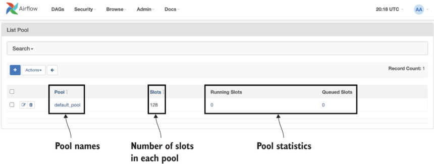
Figure 11.8 Overview of Airflow resource pools in the web UI

Figure 11.9 Creating a new resource pool in the Airflow web UI
To make your tasks use the new resource pool, you need to assign the resource pool when creating the task.
Listing 11.29 Assigning a specific resource pool to a task
PythonOperator(
    task_id="my_task",
    ...
    pool="my_resource_pool"
)
This way, Airflow will check to see if any slots are still available in my_resource_pool before scheduling the task in a given run. If the pool still contains free slots, the scheduler will claim an empty slot (decreasing the number of available slots by one) and schedule the task for execution. If the pool does not contain any free slots, the scheduler will postpone scheduling the task until a slot becomes available.
11.4.2 Detecting long-running tasks using SLAs and alerts
In some cases, your tasks or DAG runs may take longer than usual due to unforeseen issues in the data, limited resources, and so on. Airflow allows you to monitor the behavior of your tasks using its SLA (service-level agreement) mechanism. This SLA functionality effectively allows you to assign SLA timeouts to your DAGs or tasks, in which case Airflow will warn you if any of your tasks or DAGs misses its SLA (i.e., takes longer to run than the specified SLA timeout).
At the DAG level, you can assign an SLA by passing the sla argument to the default_args of the DAG.
Listing 11.30 Assigning an SLA to all tasks in the DAG (dags/05_sla_misses.py)
from datetime import timedelta

default_args = {
    "sla": timedelta(hours=2),
    ...
}

with DAG(
    dag_id="...",
    ...
    default_args=default_args,
) as dag:
    ...
By applying a DAG-level SLA, Airflow will examine the result of each task after its execution to determine whether the task’s start or end time exceeded the SLA (compared to the start time of the DAG). If the SLA was exceeded, Airflow will generate an SLA miss alert, notifying users it was missed. After generating the alert, Airflow will continue executing the rest of the DAG, generating similar alerts for other tasks that exceed the SLA.
By default, SLA misses are recorded in the Airflow metastore and can be viewed using the web UI under Browse > SLA misses. Alert emails are also sent to any email addresses defined on the DAG (using the email DAG argument), warning users that the SLA was exceeded for the corresponding task.
You can also define custom handlers for SLA misses by passing a handler function to the DAG using the sla_miss_callback parameter.
Listing 11.31 Custom callback for SLA misses (dags/05_sla_misses.py)
def sla_miss_callback(context):
    send_slack_message("Missed SLA!")

...

with DAG(
    ...
    sla_miss_callback=sla_miss_callback
) as dag:
    ...
It is also possible to specify task-level SLAs by passing an sla argument to a task’s operator.
Listing 11.32 Assigning an SLA to specific tasks
PythonOperator(
    ...
    sla=timedelta(hours=2)
)
This will only enforce the SLA for the corresponding tasks. However, it’s important to note that Airflow will still compare the end time of the task to the start time of the DAG when enforcing the SLA, rather than the start time of the task. This is because Airflow SLAs are always defined relative to the start time of the DAG, not to individual tasks.
Summary
-
Adopting common style conventions together with supporting linting/formatting tools can greatly increase the readability of your DAG code.
-
Factory methods allow you to efficiently generate recurring DAGs or task structures while capturing differences between instances in small configuration objects or files.
-
Idempotent and deterministic tasks are key to building reproducible tasks and DAGs, which are easy to rerun and backfill from within Airflow. Concepts from functional programming can help you design tasks with these characteristics.
-
Data processes can be implemented efficiently by carefully considering how data is handled (i.e., processing in the appropriate systems, limiting the amount of data that is loaded, and using incremental loading) and by caching intermediate data sets in available file systems that are available across workers.
-
You can manage/limit access to your resources in Airflow using resource pools.
-
Long-running tasks/DAGs can be detected and flagged using SLAs.
1.This can be considered to be a strength or weakness of pylint, depending on your preferences, as some people consider it overly pedantic.
2.Assuming Airflow has been configured securely. See chapters 12 and 13 for more information on configuring Airflow deployments and security in Airflow.
3.Note that you should be careful to not store any sensitive secrets in such configuration files, as these are typically stored in plain text. If you do store sensitive secrets in configuration files, make sure that only the correct people have permissions to access the file. Otherwise, consider storing secrets in more secure locations such as the Airflow metastore.
4.Note that fetching Variables like this in the global scope of your DAG is generally bad for the performance of your DAG. Read the next subsection to find out why.