This chapter covers

• Showing how data pipelines can be represented in workflows as graphs of tasks
• Understanding how Airflow fits into the ecosystem of workflow managers
• Determining if Airflow is a good fit for you

People and companies are continuously becoming more data-driven and are developing data pipelines as part of their daily business. Data volumes involved in these business processes have increased substantially over the years, from megabytes per day to gigabytes per minute. Though handling this data deluge may seem like a considerable challenge, these increasing data volumes can be managed with the appropriate tooling.

This book focuses on Apache Airflow, a batch-oriented framework for building data pipelines. Airflow’s key feature is that it enables you to easily build scheduled data pipelines using a flexible Python framework, while also providing many building blocks that allow you to stitch together the many different technologies encountered in modern technological landscapes.

Airflow is best thought of as a spider in a web: it sits in the middle of your data processes and coordinates work happening across the different (distributed) systems. As such, Airflow is not a data processing tool in itself but orchestrates the different components responsible for processing your data in data pipelines.

In this chapter, we’ll first give you a short introduction to data pipelines in Apache Airflow. Afterward, we’ll discuss several considerations to keep in mind when evaluating whether Airflow is right for you and demonstrate how to make your first steps with Airflow.

1.1 Introducing data pipelines

Data pipelines generally consist of several tasks or actions that need to be executed to achieve the desired result. For example, say we want to build a small weather dashboard that tells us what the weather will be like in the coming week (figure 1.1). To implement this live weather dashboard, we need to perform something like the following steps:

1. Fetch weather forecast data from a weather API.

2. Clean or otherwise transform the fetched data (e.g., converting temperatures from Fahrenheit to Celsius or vice versa), so that the data suits our purpose.

3. Push the transformed data to the weather dashboard.

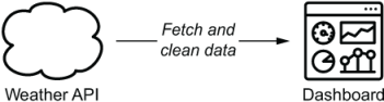
Figure 1.1 Overview of the weather dashboard use case, in which weather data is fetched from an external API and fed into a dynamic dashboard

As you can see, this relatively simple pipeline already consists of three different tasks that each perform part of the work. Moreover, these tasks need to be executed in a specific order, as it (for example) doesn’t make sense to try transforming the data before fetching it. Similarly, we can’t push any new data to the dashboard until it has undergone the required transformations. As such, we need to make sure that this implicit task order is also enforced when running this data process.

1.1.1 Data pipelines as graphs

One way to make dependencies between tasks more explicit is to draw the data pipeline as a graph. In this graph-based representation, tasks are represented as nodes in the graph, while dependencies between tasks are represented by directed edges between the task nodes. The direction of the edge indicates the direction of the dependency, with an edge pointing from task A to task B, indicating that task A needs to be completed before task B can start. Note that this type of graph is generally called a directed graph, due to the directions in the graph edges.

Applying this graph representation to our weather dashboard pipeline, we can see that the graph provides a relatively intuitive representation of the overall pipeline (figure 1.2). By just quickly glancing at the graph, we can see that our pipeline consists of three different tasks, each corresponding to one of the tasks outlined. Other than this, the direction of the edges clearly indicates the order in which the tasks need to be executed: we can simply follow the arrows to trace the execution.

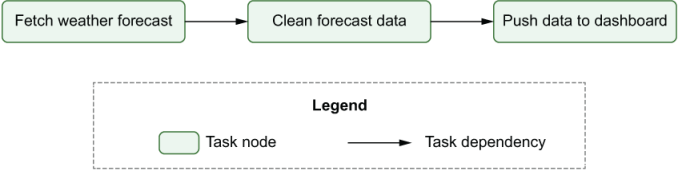
Figure 1.2 Graph representation of the data pipeline for the weather dashboard. Nodes represent tasks and directed edges represent dependencies between tasks (with an edge pointing from task A to task B, indicating that task A needs to be run before task B).

This type of graph is typically called a directed acyclic graph (DAG), as the graph contains directed edges and does not contain any loops or cycles (acyclic). This acyclic property is extremely important, as it prevents us from running into circular dependencies (figure 1.3) between tasks (where task A depends on task B and vice versa). These circular dependencies become problematic when trying to execute the graph, as we run into a situation where task 2 can only execute once task 3 has been completed, while task 3 can only execute once task 2 has been completed. This logical inconsistency leads to a deadlock type of situation, in which neither task 2 nor 3 can run, preventing us from executing the graph.

Figure 1.3 Cycles in graphs prevent task execution due to circular dependencies. In acyclic graphs (top), there is a clear path to execute the three different tasks. However, in cyclic graphs (bottom), there is no longer a clear execution path due to the interdependency between tasks 2 and 3.

Note that this representation is different from cyclic graph representations, which can contain cycles to illustrate iterative parts of algorithms (for example), as are common in many machine learning applications. However, the acyclic property of DAGs is used by Airflow (and many other workflow managers) to efficiently resolve and execute these graphs of tasks.

1.1.2 Executing a pipeline graph

A nice property of this DAG representation is that it provides a relatively straightforward algorithm that we can use for running the pipeline. Conceptually, this algorithm consists of the following steps:

1. For each open (= uncompleted) task in the graph, do the following:

   • For each edge pointing toward the task, check if the “upstream” task on the other end of the edge has been completed.
   • If all upstream tasks have been completed, add the task under consideration to a queue of tasks to be executed.

2. Execute the tasks in the execution queue, marking them completed once they finish performing their work.

3. Jump back to step 1 and repeat until all tasks in the graph have been completed.

To see how this works, let’s trace through a small execution of our dashboard pipeline (figure 1.4). On our first loop through the steps of our algorithm, we see that the clean and push tasks still depend on upstream tasks that have not yet been completed. As such, the dependencies of these tasks have not been satisfied, so at this point they can’t be added to the execution queue. However, the fetch task does not have any incoming edges, meaning that it does not have any unsatisfied upstream dependencies and can therefore be added to the execution queue.

Figure 1.4 Using the DAG structure to execute tasks in the data pipeline in the correct order: depicts each task’s state during each of the loops through the algorithm, demonstrating how this leads to the completed execution of the pipeline (end state)

After completing the fetch task, we can start the second loop by examining the dependencies of the clean and push tasks. Now we see that the clean task can be executed as its upstream dependency (the fetch task) has been completed. As such, we can add the task to the execution queue. The push task can’t be added to the queue, as it depends on the clean task, which we haven’t run yet.

In the third loop, after completing the clean task, the push task is finally ready for execution as its upstream dependency on the clean task has now been satisfied. As a result, we can add the task to the execution queue. After the push task has finished executing, we have no more tasks left to execute, thus finishing the execution of the overall pipeline.

1.1.3 Pipeline graphs vs. sequential scripts

Although the graph representation of a pipeline provides an intuitive overview of the tasks in the pipeline and their dependencies, you may find yourself wondering why we wouldn’t just use a simple script to run this linear chain of three steps. To illustrate some advantages of the graph-based approach, let’s jump to a slightly bigger example. In this new use case, we’ve been approached by the owner of an umbrella company, who was inspired by our weather dashboard and would like to try to use machine learning (ML) to increase the efficiency of their operation. To do so, the company owner would like us to implement a data pipeline that creates an ML model correlating umbrella sales with weather patterns. This model can then be used to predict how much demand there will be for the company’s umbrellas in the coming weeks, depending on the weather forecasts for those weeks (figure 1.5).

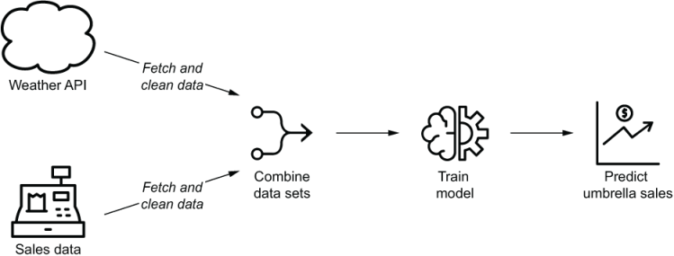
Figure 1.5 Overview of the umbrella demand use case, in which historical weather and sales data are used to train a model that predicts future sales demands depending on weather forecasts

To build a pipeline for training the ML model, we need to implement something like the following steps:

1. Prepare the sales data by doing the following:

   • Fetching the sales data from the source system
   • Cleaning/transforming the sales data to fit requirements

2. Prepare the weather data by doing the following:

   • Fetching the weather forecast data from an API
   • Cleaning/transforming the weather data to fit requirements

3. Combine the sales and weather data sets to create the combined data set that can be used as input for creating a predictive ML model.

4. Train the ML model using the combined data set.

5. Deploy the ML model so that it can be used by the business.

This pipeline can be represented using the same graph-based representation that we used before, by drawing tasks as nodes and data dependencies between tasks as edges.

One important difference from our previous example is that the first steps of this pipeline (fetching and clearing the weather/sales data) are in fact independent of each other, as they involve two separate data sets. This is clearly illustrated by the two separate branches in the graph representation of the pipeline (figure 1.6), which can be executed in parallel if we apply our graph execution algorithm, making better use of available resources and potentially decreasing the running time of a pipeline compared to executing the tasks sequentially.

Figure 1.6 Independence between sales and weather tasks in the graph representation of the data pipeline for the umbrella demand forecast model. The two sets of fetch/cleaning tasks are independent as they involve two different data sets (the weather and sales data sets). This independence is indicated by the lack of edges between the two sets of tasks.

Another useful property of the graph-based representation is that it clearly separates pipelines into small incremental tasks rather than having one monolithic script or process that does all the work. Although having a single monolithic script may not initially seem like that much of a problem, it can introduce some inefficiencies when tasks in the pipeline fail, as we would have to rerun the entire script. In contrast, in the graph representation, we need only to rerun any failing tasks (and any downstream dependencies).

1.1.4 Running pipeline using workflow managers

Of course, the challenge of running graphs of dependent tasks is hardly a new problem in computing. Over the years, many so-called “workflow management” solutions have been developed to tackle this problem, which generally allow you to define and execute graphs of tasks as workflows or pipelines.

Some well-known workflow managers you may have heard of include those listed in table 1.1.

Table 1.1 Overview of several well-known workflow managers and their key characteristics.

Name	Originated at1	Workflows defined in	Written in	Scheduling	Backfilling	User interface2	Installation platform	Horizontally scalable
Airflow	Airbnb	Python	Python	Yes	Yes	Yes	Anywhere	Yes
Argo	Applatix	YAML	Go	Third party3		Yes	Kubernetes	Yes
Azkaban	LinkedIn	YAML	Java	Yes	No	Yes	Anywhere
Conductor	Netflix	JSON	Java	No		Yes	Anywhere	Yes
Luigi	Spotify	Python	Python	No	Yes	Yes	Anywhere	Yes
Make		Custom DSL	C	No	No	No	Anywhere	No
Metaflow	Netflix	Python	Python	No		No	Anywhere	Yes
Nifi	NSA	UI	Java	Yes	No	Yes	Anywhere	Yes
Oozie		XML	Java	Yes	Yes	Yes	Hadoop	Yes

Although each of these workflow managers has its own strengths and weaknesses, they all provide similar core functionality that allows you to define and run pipelines containing multiple tasks with dependencies.

One of the key differences between these tools is how they define their workflows. For example, tools such as Oozie use static (XML) files to define workflows, which provides legible workflows but limited flexibility. Other solutions such as Luigi and Airflow allow you to define workflows as code, which provides greater flexibility but can be more challenging to read and test (depending on the coding skills of the person implementing the workflow).

Other key differences lie in the extent of features provided by the workflow manager. For example, tools such as Make and Luigi do not provide built-in support for scheduling workflows, meaning that you’ll need an extra tool like Cron if you want to run your workflow on a recurring schedule. Other tools may provide extra functionality such as scheduling, monitoring, user-friendly web interfaces, and so on built into the platform, meaning that you don’t have to stitch together multiple tools yourself to get these features.

All in all, picking the right workflow management solution for your needs will require some careful consideration of the key features of the different solutions and how they fit your requirements. In the next section, we’ll dive into Airflow—the focus of this book—and explore several key features that make it particularly suited for handling data-oriented workflows or pipelines.

1.2 Introducing Airflow

In this book, we focus on Airflow, an open source solution for developing and monitoring workflows. In this section, we’ll provide a helicopter view of what Airflow does, after which we’ll jump into a more detailed examination of whether it is a good fit for your use case.

1.2.1 Defining pipelines flexibly in (Python) code

Similar to other workflow managers, Airflow allows you to define pipelines or workflows as DAGs of tasks. These graphs are very similar to the examples sketched in the previous section, with tasks being defined as nodes in the graph and dependencies as directed edges between the tasks.

In Airflow, you define your DAGs using Python code in DAG files, which are essentially Python scripts that describe the structure of the corresponding DAG. As such, each DAG file typically describes the set of tasks for a given DAG and the dependencies between the tasks, which are then parsed by Airflow to identify the DAG structure (figure 1.7). Other than this, DAG files typically contain some additional metadata about the DAG telling Airflow how and when it should be executed, and so on. We’ll dive into this scheduling more in the next section.

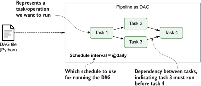
Figure 1.7 Airflow pipelines are defined as DAGs using Python code in DAG files. Each DAG file typically defines one DAG, which describes the different tasks and their dependencies. Besides this, the DAG also defines a schedule interval that determines when the DAG is executed by Airflow.

One advantage of defining Airflow DAGs in Python code is that this programmatic approach provides you with a lot of flexibility for building DAGs. For example, as we will see later in this book, you can use Python code to dynamically generate optional tasks depending on certain conditions or even generate entire DAGs based on external metadata or configuration files. This flexibility gives a great deal of customization in how you build your pipelines, allowing you to fit Airflow to your needs for building arbitrarily complex pipelines.

In addition to this flexibility, another advantage of Airflow’s Python foundation is that tasks can execute any operation that you can implement in Python. Over time, this has led to the development of many Airflow extensions that enable you to execute tasks across a wide variety of systems, including external databases, big data technologies, and various cloud services, allowing you to build complex data pipelines bringing together data processes across many different systems.

1.2.2 Scheduling and executing pipelines

Once you’ve defined the structure of your pipeline(s) as DAG(s), Airflow allows you to define a schedule interval for each DAG, which determines exactly when your pipeline is run by Airflow. This way, you can tell Airflow to execute your DAG every hour, every day, every week, and so on, or even use more complicated schedule intervals based on Cron-like expressions.

To see how Airflow executes your DAGs, let’s briefly look at the overall process involved in developing and running Airflow DAGs. At a high level, Airflow is organized into three main components (figure 1.8):

• The Airflow scheduler —Parses DAGs, checks their schedule interval, and (if the DAGs’ schedule has passed) starts scheduling the DAGs’ tasks for execution by passing them to the Airflow workers.

• The Airflow workers —Pick up tasks that are scheduled for execution and execute them. As such, the workers are responsible for actually “doing the work.”

• The Airflow webserver —Visualizes the DAGs parsed by the scheduler and provides the main interface for users to monitor DAG runs and their results.

Figure 1.8 Overview of the main components involved in Airflow (e.g., the Airflow webserver, scheduler, and workers)

The heart of Airflow is arguably the scheduler, as this is where most of the magic happens that determines when and how your pipelines are executed. At a high level, the scheduler runs through the following steps (figure 1.9):

1. Once users have written their workflows as DAGs, the files containing these DAGs are read by the scheduler to extract the corresponding tasks, dependencies, and schedule interval of each DAG.

2. For each DAG, the scheduler then checks whether the schedule interval for the DAG has passed since the last time it was read. If so, the tasks in the DAG are scheduled for execution.

3. For each scheduled task, the scheduler then checks whether the dependencies (= upstream tasks) of the task have been completed. If so, the task is added to the execution queue.

4. The scheduler waits for several moments before starting a new loop by jumping back to step 1.

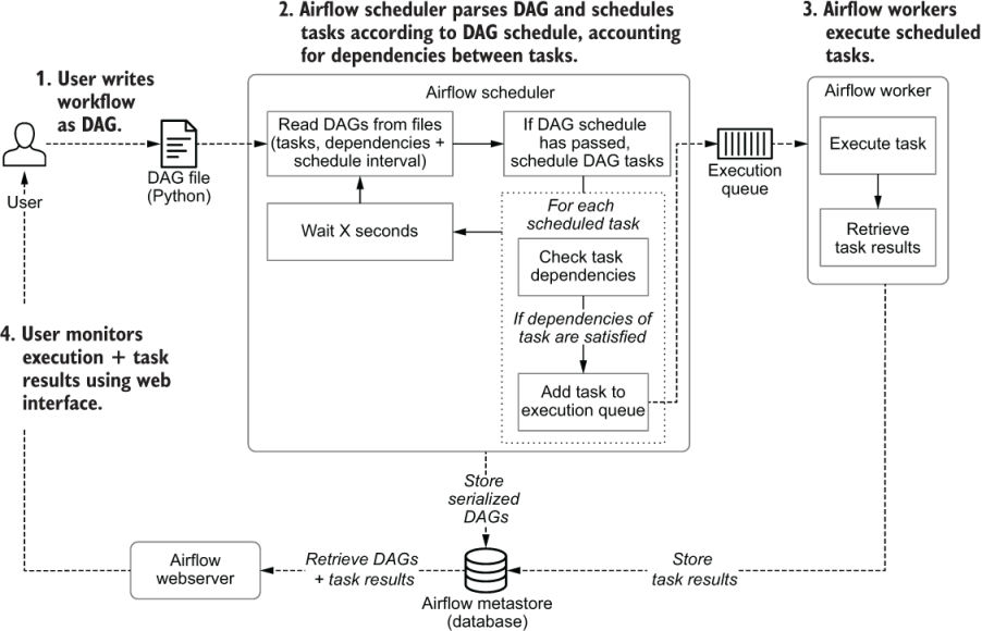
Figure 1.9 Schematic overview of the process involved in developing and executing pipelines as DAGs using Airflow

The astute reader might have noticed that the steps followed by the scheduler are, in fact, very similar to the algorithm introduced in section 1.1. This is not by accident, as Airflow is essentially following the same steps, adding some extra logic on top to handle its scheduling logic.

Once tasks have been queued for execution, they are picked up by a pool of Airflow workers that execute tasks in parallel and track their results. These results are communicated to Airflow’s metastore so that users can track the progress of tasks and view their logs using the Airflow web interface (provided by the Airflow webserver).

1.2.3 Monitoring and handling failures

In addition to scheduling and executing DAGs, Airflow also provides an extensive web interface that can be used for viewing DAGs and monitoring the results of DAG runs. After you log in (figure 1.10), the main page provides an extensive overview of the different DAGs with summary views of their recent results (figure 1.11).

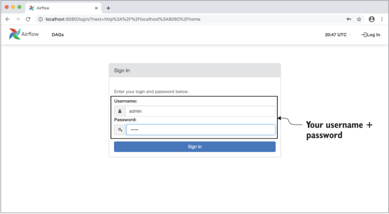
Figure 1.10 The login page for the Airflow web interface. In the code examples accompanying this book, a default user “admin” is provided with the password “admin.”

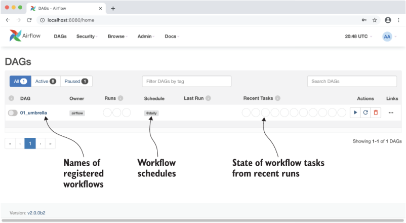
Figure 1.11 The main page of Airflow’s web interface, showing an overview of the available DAGs and their recent results

For example, the graph view of an individual DAG provides a clear overview of the DAG’s tasks and dependencies (figure 1.12), similar to the schematic overviews we’ve been drawing in this chapter. This view is particularly useful for viewing the structure of a DAG (providing detailed insight into dependencies between tasks), and for viewing the results of individual DAG runs.

Figure 1.12 The graph view in Airflow’s web interface, showing an overview of the tasks in an individual DAG and the dependencies between these tasks

Besides this graph view, Airflow also provides a detailed tree view that shows all running and historical runs for the corresponding DAG (figure 1.13). This is arguably the most powerful view provided by the web interface, as it gives you a quick overview of how a DAG has performed over time and allows you to dig into failing tasks to see what went wrong.

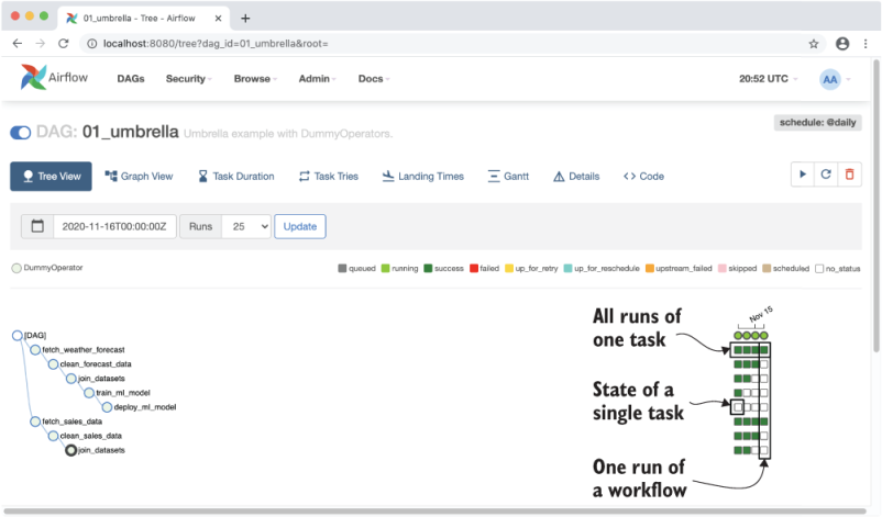
Figure 1.13 Airflow’s tree view, showing the results of multiple runs of the umbrella sales model DAG (most recent + historical runs). The columns show the status of one execution of the DAG and the rows show the status of all executions of a single task. Colors (which you can see in the e-book version) indicate the result of the corresponding task. Users can also click on the task “squares” for more details about a given task instance, or to reset the state of a task so that it can be rerun by Airflow, if desired.

By default, Airflow can handle failures in tasks by retrying them a couple of times (optionally with some wait time in between), which can help tasks recover from any intermittent failures. If retries don’t help, Airflow will record the task as being failed, optionally notifying you about the failure if configured to do so. Debugging task failures is pretty straightforward, as the tree view allows you to see which tasks failed and dig into their logs. The same view also enables you to clear the results of individual tasks to rerun them (together with any tasks that depend on that task), allowing you to easily rerun any tasks after you make changes to their code.

1.2.4 Incremental loading and backfilling

One powerful feature of Airflow’s scheduling semantics is that the schedule intervals not only trigger DAGs at specific time points (similar to, for example, Cron), but also provide details about the last and (expected) next schedule intervals. This essentially allows you to divide time into discrete intervals (e.g., every day, week, etc.), and run your DAG for each of these intervals.⁴

This property of Airflow’s schedule intervals is invaluable for implementing efficient data pipelines, as it allows you to build incremental data pipelines. In these incremental pipelines, each DAG run processes only data for the corresponding time slot (the data’s delta) instead of having to reprocess the entire data set every time. Especially for larger data sets, this can provide significant time and cost benefits by avoiding expensive recomputation of existing results.

Schedule intervals become even more powerful when combined with the concept of backfilling, which allows you to execute a new DAG for historical schedule intervals that occurred in the past. This feature allows you to easily create (or backfill ) new data sets with historical data simply by running your DAG for these past schedule intervals. Moreover, by clearing the results of past runs, you can also use this Airflow feature to easily rerun any historical tasks if you make changes to your task code, allowing you to easily reprocess an entire data set when needed.

1.3 When to use Airflow

After this brief introduction to Airflow, we hope you’re sufficiently enthusiastic about getting to know Airflow and learning more about its key features. However, before going any further, we’ll first explore several reasons you might want to choose to work with Airflow (as well as several reasons you might not), to ensure that Airflow is indeed the best fit for you.

1.3.1 Reasons to choose Airflow

In the past sections, we’ve already described several key features that make Airflow ideal for implementing batch-oriented data pipelines. In summary, these include the following:

• The ability to implement pipelines using Python code allows you to create arbitrarily complex pipelines using anything you can dream up in Python.

• The Python foundation of Airflow makes it easy to extend and add integrations with many different systems. In fact, the Airflow community has already developed a rich collection of extensions that allow Airflow to integrate with many different types of databases, cloud services, and so on.

• Rich scheduling semantics allow you to run your pipelines at regular intervals and build efficient pipelines that use incremental processing to avoid expensive recomputation of existing results.

• Features such as backfilling enable you to easily (re)process historical data, allowing you to recompute any derived data sets after making changes to your code.

• Airflow’s rich web interface provides an easy view for monitoring the results of your pipeline runs and debugging any failures that may have occurred.

An additional advantage of Airflow is that it is open source, which guarantees that you can build your work on Airflow without getting stuck with any vendor lock-in. Managed Airflow solutions are also available from several companies (should you desire some technical support), giving you a lot of flexibility in how you run and manage your Airflow installation.

1.3.2 Reasons not to choose Airflow

Although Airflow has many rich features, several of Airflow’s design choices may make it less suitable for certain cases. For example, some use cases that are not a good fit for Airflow include the following:

• Handling streaming pipelines, as Airflow is primarily designed to run recurring or batch-oriented tasks, rather than streaming workloads.

• Implementing highly dynamic pipelines, in which tasks are added/removed between every pipeline run. Although Airflow can implement this kind of dynamic behavior, the web interface will only show tasks that are still defined in the most recent version of the DAG. As such, Airflow favors pipelines that do not change in structure every time they run.

• Teams with little or no (Python) programming experience, as implementing DAGs in Python can be daunting with little Python experience. In such teams, using a workflow manager with a graphical interface (such as Azure Data Factory) or a static workflow definition may make more sense.

• Similarly, Python code in DAGs can quickly become complex for larger use cases. As such, implementing and maintaining Airflow DAGs require proper engineering rigor to keep things maintainable in the long run.

Also, Airflow is primarily a workflow/pipeline management platform and does not (currently) include more extensive features such as maintaining data lineages, data versioning, and so on. Should you require these features, you’ll probably need to look at combining Airflow with other specialized tools that provide those capabilities.

1.4 The rest of this book

By now you should (hopefully) have a good idea of what Airflow is and how its features can help you implement and run data pipelines. In the remainder of this book, we’ll begin by introducing the basic components of Airflow that you need to be familiar with to start building your own data pipelines. These first few chapters should be broadly applicable and appeal to a wide audience. For these chapters, we expect you to have intermediate experience with programming in Python (~one year of experience), meaning that you should be familiar with basic concepts such as string formatting, comprehensions, args/kwargs, and so on. You should also be familiar with the basics of the Linux terminal and have a basic working knowledge of databases (including SQL) and different data formats.

After this introduction, we’ll dive deeper into more advanced features of Airflow such as generating dynamic DAGs, implementing your own operators, running containerized tasks, and so on. These chapters will require some more understanding of the involved technologies, including writing your own Python classes, basic Docker concepts, file formats, and data partitioning. We expect this second part to be of special interest to the data engineers in the audience.

Finally, several chapters toward the end of the book focus on topics surrounding the deployment of Airflow, including deployment patterns, monitoring, security, and cloud architectures. We expect these chapters to be of special interest for people interested in rolling out and managing Airflow deployments, such as system administrators and DevOps engineers.

Summary

• Data pipelines can be represented as DAGs, which clearly define tasks and their dependencies. These graphs can be executed efficiently, taking advantage of any parallelism inherent in the dependency structure.

• Although many workflow managers have been developed over the years for executing graphs of tasks, Airflow has several key features that makes it uniquely suited for implementing efficient, batch-oriented data pipelines.

• Airflow consists of three core components: the webserver, the scheduler, and the worker processes, which work together to schedule tasks from your data pipelines and help you monitor their results.

---

^1. Some tools were originally created by (ex-)employees of a company; however, all tools are open sourced and not represented by one single company.

^2. The quality and features of user interfaces vary widely.

^3. https://github.com/bitphy/argo-cron.

^4.If this sounds a bit abstract to you now, don’t worry, as we provide more detail on these concepts later in the book.