9
Shrinkage

In this chapter we present a famous result due to Stein (1955) and further elaborated by James & Stein (1961). It concerns estimating several parameters as part of the same decision problem. Let x = (x₁, ..., x_p)′ be distributed according to a multivariate p-dimensional N(θ, I) distribution, and assume the multivariate quadratic loss function

The estimator δ(x) = x is the maximum likelihood estimator of θ, it is unbiased, and it has the smallest risk among all unbiased estimators. This would make it the almost perfect candidate from a frequentist angle. It is also the formal Bayes rule if one wishes to specify an improper flat prior on θ. However, Stein showed that such an estimator is not admissible. Oops.

Robert describes the aftermath as follows:

Efron adds:

The Stein effect occurs even though the dimensions are unrelated, and it can be explained primarily through the joint loss , which allows the dominating estimator to “borrow strength” across dimensions, and bring individual estimates closer together, trading off errors in one dimension with those in another. This is usually referred to as shrinkage.

Our goal here is to build some intuition for the main results, and convey a sense for which approaches weather the storm in reasonable shape. In the end these include Bayes, but also empirical Bayes and some varieties of minimax. We first present the James–Stein theorem, straight up, no chaser, in the simplest form we know. We then look at some of the most popular attempts at intuitive explanations, and finally turn to more general formulations, both Bayes and minimax.

Featured article:

Stein, C. (1955). Inadmissibility of the usual estimator for the mean of a multivariate normal distribution, Proceedings of the Third Berkeley Symposium on Mathematical Statistics and Probability 1: 197–206.

The literature on shrinkage, its justifications and ramifications, is vast. For a more detailed discussion we refer to Berger (1985), Brandwein and Strawderman (1990), Robert (1994), and Schervish (1995) and the references therein.

9.1 The Stein effect

Theorem 9.1 Suppose that a p-dimensional vector x = (x₁, x₂, ..., x_p)′ follows a multivariate normal distribution with mean vector θ = (θ₁, ..., θ_p)′ and the identity covariance matrix I. Let A = Θ = ℜ^p, and let the loss be . Then, for p > 2, the decision rule

dominates δ(x) = x.

Proof: The risk function of δ is

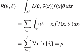
To compute the risk function of δ^JS we need two expressions:

where y follows a Poisson distribution with mean . We will prove these results later. First, let us see how these can be used to get us to the finish line:

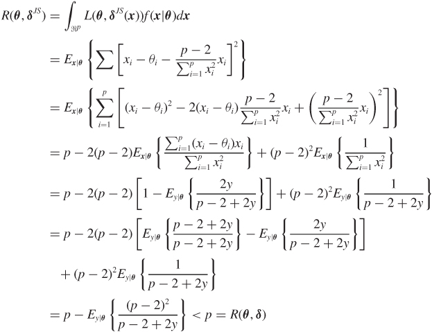
and the theorem is proved.

Now on to the two expectations in equations (9.2) and (9.3). See also James and Stein (1961), Baranchik (1973), Arnold (1981), or Schervish (1995, pp. 163–167). We will first prove equation (9.3). A random variable U with a noncentral chi-square distribution with k degrees of freedom and noncentrality parameter λ is a mixture with conditional distributions U|Y = y having a central chi-square distribution with k + 2y degrees of freedom and where the mixing variable Y has a Poisson distribution with mean λ. In our problem, has a noncentral chi-square distribution with p degrees of freedom and noncentrality parameter equal to . Using the mixture representation of the noncentral chi-square, with and , we get

The last equality is based on the expression for the mean of a central inverse chi-square distribution.

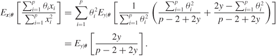
Next, to prove equation (9.2) we will use the following result:

The proof is left as an exercise (Problem 9.4). Now,

Note that

Thus,

The assumption of unit variance is convenient but not required—any known p-dimensional vector of variances would lead to the same result as we can standardize the observations. For the same reason, as long as the variance(s) are known, x itself could be a vector of sample means.

The estimator δ^JS in Theorem 9.1 is the James–Stein estimator. It is a shrinkage estimator in that, in general, the individual components of δ are closer to 0 than the corresponding components of x, so the p-dimensional vector of observations is said to be shrunk towards 0.

How does the James–Stein estimator itself behave under the admissibility criterion? It turns out that it too can be dominated. For example, the so-called truncated James–Stein estimator

is a variant that never switches the sign of an observation, and does dominate δ^JS. Here the subscript + denotes the positive part of the expression in the square brackets. Put more simply, when the stuff in these brackets is negative we replace it with 0. This estimator is itself inadmissible. One way to see this is to use a complete class result due to Sacks (1963), who showed that any admissible estimate can be represented as a formal Bayes rule of the form

These estimators are analytic in x while the positive part estimator is continuous but not differentiable. Baranchik (1970) also provided an estimator which dominates the James–Stein estimator. The James–Stein estimator is important for having revealed a weakness of standard approaches and for having pointed to shrinkage as an important direction for improvement. However, direct applications have not been numerous, perhaps because it is not difficult to find more intuitive, or better performing, implementations.

9.2 Geometric and empirical Bayes heuristics

9.2.1 Is x too big for θ?

An argument that is often heard as “intuitive” support for the need to shrink is captured by Figure 9.1. Stein would mention it in his lectures, and many have reported it since. The story goes more or less like this. In the setting of Theorem 9.1, because E_x|θ[(x–θ)′θ] = 0, we expect orthogonality between x–θ and θ. Moreover, because E_x|θ[x′x] = p + θ′θ, it may appear that x is too big as an estimator of θ and thus that it may help to shorten it. For example, the projection of θ on x might be closer. However, the projection (1 – a) x depends on θ through a. Therefore, we need to estimate a. Assuming that (i) the angle between θ and x – θ is right, (ii) x′x is close to its expected value, θ′θ + p, and (iii) (x – θ)′(x – θ) is close to its expected value p, then using Pythagoras’s theorem in the right subtriangles in Figure 9.1 we obtain

Figure 9.1 Geometric heuristic for the need to shrink. Vectors here live in p-dimensional spaces. Adapted with minor changes from Brandwein and Strawderman (1990).

and

By equating the above expressions, is an estimate of a. Thus, an estimator for θ would be

similar to the James–Stein estimator introduced in Section 9.1.

While this heuristic does not have any pretense of rigor, it is suggestive. However, a doubt remains about how much insight can be gleaned from the emphasis placed on the origin as the shrinkage point. For example, Efron (1978) points out that if one specifies an arbitrary origin x₀ and defines the estimator

to shrink towards the x₀ instead of 0, this estimator also dominates x. Berger (1985) has details and references for various implementations of this idea. For many choices of x₀ the heuristic we described breaks down, but the Stein effect still works.

One way in which the insight of Figure 9.1 is sometimes summarized is by saying that “θ is closer to 0 than x.” Is this reasonable? Maybe. But then shrinkage works for every x₀. It certainly seems harder to claim that “θ is closer to x₀ than x” irrespective of what x₀ is. Similarly, some skepticism is probably useful when considering heuristics based on the fact that the probability that x′x > θ′θ can be quite large even for relatively small p and large θ. Of course this is true, but it is less clear whether this is why shrinkage works. For more food for thought, observe that, overall, shrinkage is more pronounced when the data x are closer to the origin. Perhaps a more useful perspective is that of “borrowing strength” across dimensions, and shrinking when dimensions look similar. This is made formal in the Bayes and empirical Bayes approaches considered next.

9.2.2 Empirical Bayes shrinkage

The idea behind empirical Bayes approaches is to estimate the prior empirically. When one has a single estimation problem this is generally quite hard, but when a battery of problems are considered together, as is the case in this chapter, this is possible, and often quite useful. The earliest example is due to Robbins (1956) while Efron and Morris highlighted the relevance of this approach for shrinkage and for the so-called hierarchical models (Efron and Morris 1973b, Efron and Morris 1973a).

A relatively general formulation could go as follows. The p-dimensional observation vector x has distribution f(x|θ), while parameters θ have distribution π(θ|τ) with τ unknown and of dimension generally much lower than p. A classic example is one where x_i represents a noisy measurement of θ_i—say, the observed and real weight of a tree. The distribution π(θ|τ) describes the variation of the unobserved true measurements across the population. This model is an example of a multilevel model, with one level representing the noise in the measurements and the other the population variation. Depending on the study design, the θ may be called random effects. Multilevel models are now a mainstay of applied statistics and the primary venue for shrinkage in practical applications (Congdon 2001, Ferreira and Lee 2007).

If interest is in θ, an empirical Bayes estimator can be obtained by deriving the marginal likelihood

and using it to identify a reasonable estimator of τ, say . This estimator is then plugged back into π, so that a prior is now available for use, via the Bayes rule, to obtain the Bayes estimator for θ. Under squared error loss this is

An empirical Bayes analysis does not correspond to a coherent Bayesian updating, since the data are used twice, but it has nice properties that contributed to its wide use.

While we use the letter π for the distribution of θ given τ, this distribution is a somewhat intermediate creation between a prior and a likelihood: its interpretation can vary significantly with the context, and it can be empirically estimable in some problems. A Bayesian analysis of this model would also assign a prior to τ, and proceed with coherent updating and expected loss minimization as in Theorem 7.1. If p is large and the likelihood is more concentrated than the prior, that is the noise is small compared to the variation across the population, the Bayes and empirical Bayes estimators of θ will be close.

Returning to our p-dimensional vector x from a multivariate normal distribution with mean vector θ and covariance matrix I, we can derive easily an empirical Bayes estimator as follows. Assume that a priori . The Bayes estimator of θ, under a quadratic loss function, is the posterior mean, that is

assuming is fixed. The empirical Bayes estimator of θ is found as follows. First, we find the unconditional distribution of x which is, in this case, normal with mean 0 and variance . Second, we find a reasonable estimator for τ₀. Actually, in this case, it makes sense to aim directly at the shrinkage factor . Because

and

then is an unbiased estimator of . Plugging this directly into equation (9.8) gives the empirical Bayes estimator

This is the James–Stein estimator! We can reinterpret it as a weighted average between a prior mean of 0 and an observed measurement x, with weights that are learned completely from the data. The prior mean does not have to be zero: in fact versions of this where one shrinks towards the empirical average of x can also be shown to dominate the MLE, and to have an empirical Bayes justification.

Instead of using an unbiased estimator of the shrinkage factor, one could, alternatively, find an estimator for τ² using the maximum likelihood approach, which leads to

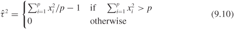
and the corresponding empirical Bayes estimator is

similar to the estimator of equation (9.5).

9.3 General shrinkage functions

9.3.1 Unbiased estimation of the risk of x + g(x)

Stein developed a beautiful way of providing insight into the subtle issues raised in this chapter, by setting very general conditions for estimators of the form δ_g(x) = x + g(x) to dominate δ(x) = x. We begin with two preparatory lemmas. All the results in this section are under the assumptions of Theorem 9.1.

Lemma 1 Let y be distributed as a N(θ,1). Let h be the indefinite integral of a measurable function h′ such that

Then

Proof: Starting from the left hand side,

Assumption (9.13) is used in the integration by parts.

Weaker versions of assumption (9.13) are used in Stein (1981). Incidentally, the converse of this lemma is also true, so if equation (9.14) holds for all reasonable h, then y must be normal.

The next lemma cranks this result up to p dimensions, and looks at the covariance between the error x – θ and the shrinkage function g(x). It requires a technical differentiability condition and some more notation: a function h : ℜ^p → ℜ is almost differentiable if there exists a function ∇h : ℜ^p → ℜ^p such that

where z is in ℜ^p and ∇ can also be thought of as the vector differential operator

A function g : ℜ^p → ℜ^p is almost differentiable if every coordinate is.

Lemma 2 If h is almost differentiable and E_x|θ[(∇h(x))′(∇h(x))] < ∞, then

Using these two lemmas, the next theorem provides a usable closed form for the risk of estimators of the form δ_g(x) = x + g(x). Look at Stein (1981) for proofs.

Theorem 9.2 (Unbiased estimation of risk) If g : ℜ^p → ℜ^p is almost differentiable and such that

then

The risk is decomposable into the risk of the estimator x plus a component that depends on the shrinkage function g. A corollary of this result, and the key of our exercise, is that if we can specify g so that

for all values of x (with at least a strict inequality somewhere), then δ_g(x) dominates δ(x) = x. This argument encapsulates the bias–variance trade-off in shrinkage estimators: shrinkage works when the negative covariance between errors x – θ and corrections g(x) more than offsets the bias induced by g(x). Because of the additivity of the losses across dimensions, we can trade off bias in one dimension for variance in another. This aspect more than any other sets the Stein estimation setting apart from problems with a single parameter of interest.

Before we move to discussing ways to choose g, note that the right hand side of equation (9.17) is the risk of δ_g, so the quantity

is an unbiased estimator of the unknown R(δ_g, θ). The technique of finding an unbiased estimator of the risk directly can be useful in general. Stein, for example, suggests that it could be used for choosing estimators that, after the data are observed, have small estimated risk. More discussion appears in Stein (1981).

9.3.2 Bayes and minimax shrinkage

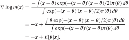
There is a solid connection between estimators like δ_g and Bayes rules. As usual, call m(x) the marginal density of x, that is m(x) = ∫f(x|θ)π(θ)dθ. Then it turns out that, using the gradient representation,

E[θ|x] = x + ∇ log m(x).

This is because

Thus setting g(x) = ∇ log m(x), for some prior π, is a very promising choice of g, as are, more generally, functions m from ℜ^p to the positive real line. When we restrict attention to these, the condition for dominance given in inequality (9.18) becomes, after a little calculus,

Thus, to produce an estimator that dominates x it is enough to find a function m with or ∇²m(x) ≤ 0—the latter are called superharmonic functions.

If we do not require that m(x) is a proper density, we can choose m(x) = |x|^−(p−2). For p > 2 this is a superharmonic function and ∇ log m(x) = −x(p – 2)/x′x, so it yields the James–Stein estimator of Theorem 9.1.

The estimator δ^M(x) = x is a minimax rule, but it is not the only minimax rule. Any rule whose risk is bounded by p will also be minimax, so it is not too difficult to concoct shrinkage approaches that are minimax. This has been a topic of great interest, and the literature is vast. Our brief discussion is based on a review by Brandwein and Strawderman (1990), which is also a perfect entry point if you are interested in more.

A good starting point is the James–Stein estimator δ^JS, which is minimax, because its risk is bounded by p. Can we use the form of δ^JS to motivate a broader class of minimax estimators? This result is an example:

Theorem 9.3 If h is a monotone increasing function such that 0 ≤ h ≤ 2(p – 2), then the estimator

is minimax.

Proof: In this proof we assume that h(x′x)/x′x follows the conditions stated in Lemma 1. Then, by applying Lemma 1,

The above inequality follows from the fact that h is positive and increasing, which implies h′ ≥ 0. Moreover, by assumption,

0 ≤ h(x′x) ≤ 2(p – 2),

which implies that for nonnull vectors x,

Therefore,

By combining inequalities (9.19) and (9.20) above we conclude that the risk of this estimator is

In Section 7.7 we proved that x is minimax and it has constant risk p. Since the risk of δ^M is at most p, it is minimax.

The above lemma gives us a class of shrinkage estimators. The Bayes and generalized Bayes estimators may be found in this class. Consider a hierarchical model defined as follows: conditional on λ, θ is distributed as N(0,(1 – λ)/λI). Also, λ ~ (1 – b)λ^−b for 0 ≤ b < 1. The Bayes estimator is the posterior mean of θ given by

The next theorem gives conditions under which the Bayes estimator given by (9.21) is minimax.

Theorem 9.4

1. For p ≥ 5, the proper Bayes estimator δ* from (9.21) is minimax as long as b ≥ (6 – p)/2.

2. For p ≥ 3, the generalized Bayes estimator δ* from (9.21) is minimax if (6 – p)/2 ≤ b < (p + 2)/2.

Proof: One can show that the posterior mean of λ is

where h(x′x) is the term in square brackets on the right side of expression (9.22).

Observe that h(^x′x) ≤ p + 2 – 2b. Moreover, it is monotone increasing because is increasing. Application of Theorem 9.3 completes the proof.

We saw earlier that the Bayes rules, under very general conditions, can be written as x + ∇ log m(x), and that a sufficient condition for these rules to dominate δ is that m be superharmonic. It is therefore no surprise that we have the following theorem.

Theorem 9.5 If π(θ) is superharmonic, then x + ∇ log m(x) is minimax.

This theorem provides a broader intersection of the Bayes and minimax shrinkage approaches.

9.4 Shrinkage with different likelihood and losses

A Stein effect can also be observed when considering different sampling distributions as well as different loss functions. Brown (1975) discusses inadmissibility of the mean under whole families of loss functions.

On the likelihood side an important generalization is to the case of unknown variance. Stein (1981) discusses an extension of the results presented in this chapter using the unbiased estimation of risk technique. More broadly, spherically symmetric distributions are distributions with density f((x – θ)′(x – θ)) in ℜ^p. When p > 2, δ(x) = x is inadmissible when estimating θ with any of these distributions. Formally we have:

Theorem 9.6 Let z = (x, y) in ℜ^p, with distribution

z ~ f((x – θ)′(x – θ) + y′y),

and x ∊ ℜ^q, y ∊ ℜ^p−q. The estimator

δ_h(z) = (1 – h(x′x, y′y))x

dominates δ(x) = x under quadratic loss if there exist α, β > 0 such that:

1. t^αh(t, u) is a nondecreasing function of t for every u;

2. u^−β h(t, u) is a nonincreasing function of u for every t; and

3. 0 ≤ (t/u)h(t, u) ≤ 2(q – 2)α/(p – q – 2 + 4β).

For details on the proof see Robert (1994, pp. 67–68). Moreover, the Stein effect is robust in the class of spherically symmetric distributions with finite quadratic risk since the conditions on h do not depend on f.

In discrete data problems, there are, however, significant exceptions. For example, Alam (1979) and Brown (1981) show that the maximum likelihood estimator is admissible for estimating several binomial parameters under squared error loss. Also, the MLE is admissible for a vector of multinomial probabilities and a variety of other discrete problems.

9.5 Exercises

Problem 9.1 Consider a sample

x = (x₁, 0, 6, 5, 9, 0, 13, 0, 26, 1, 3, 0, 0, 4, 0, 34, 21, 14, 1, 9)′

where each x_i ~ Poi(λ_i). Let δ^EB denote the 20-dimensional empirical Bayes decision rule for estimating the vector λ under squared error loss and let be the first coordinate, that is the estimate of λ₁.

Write a computer program to plot versus x₁ assuming the following prior distributions:

1. λ_i ~ Exp(1), i = 1, ..., 20

2. λ_i ~ Exp(γ), i = 1, ..., 20, γ > 0

3. λ_i ~ Exp(γ), i = 1, ..., 20, γ either 1 or 10

4. λ_i ~ (1 – α)I₀ + α Exp(γ), α ∊ (0, 1), γ > 0,

where Exp(γ) is an exponential with mean 1/γ.

Write a computer program to graph the risk functions corresponding to each of the choices above, as you vary λ₁ and fix the other coordinates λ_i = x_i, i ≥ 2.

Problem 9.2 If x is a p-dimensional normal with mean θ and identity covariance matrix, and g is a continuous piecewise continuously differentiable function from ℜ^p to ℜ^p satisfying

then

E_x|θ[(x + g(x) – θ)′(x + g(x) – θ)] = p + E_x|θ[g(x)′g(x) + 2∇′g(x)],

where ∇ is the vector differential operator with coordinates

You can take this result for granted.

Consider the estimator

δ(x) = x + g(x)

where

where z is the vector of order statistics of x, and

This estimator is discussed in Stein (1981).

Questions:

1. Why would anyone ever want to use this estimator?

2. Using the result above, show that the risk is

   

3. Find a vector θ for which this estimator has lower risk than the James–Stein estimator.

Problem 9.3 For p = 10, graph the risk of the two empirical Bayes estimators of Section 9.2.2 as a function of θ′θ.

Problem 9.4 Prove equation (9.4) using the assumptions of Theorem 9.1.

Problem 9.5 Construct an estimator with the following two properties:

1. δ is the limit of a sequence of Bayes rules as a hyperparamter gets closer to its extreme.

2. δ is not admissible.

You do not need to look very far.