7
Decision functions

This chapter reviews the architecture of statistical decision theory—a formal attempt at providing a rational foundation to the way we learn from data. Our overview is broad, and covers concepts developed over several decades and from different viewpoints. The seed of the ideas we present, as Ferguson (1976) points out, can be traced back to Bernoulli (1738), Laplace (1812), and Gauss (1821). During the late 1880s, an era when the utilitarianism of Bentham and Mill had a prominent role in economics and social sciences, Edgeworth commented:

This idea was made formal and general through the conceptual framework known today as statistical decision theory, due essentially to Abraham Wald (Wald 1945, Wald 1949). Historical and biographical details are in Weiss (1992). In his 1949 article on statistical decision functions, a prelude to a book of the same title to appear in 1950, Wald proposed a unifying framework for much of the existing statistical theory, based on treating statistical inference as a special case of game theory. A mathematical theory of games that provided the foundation for economic theory had been proposed by von Neumann and Morgenstern in the same 1944 book that contained the axiomatization of utility theory discussed in Chapter 3. Wald framed statistical inference as a two-person, zero-sum game. One of the players is Nature and the other player is the Statistician. Nature chooses the probability distribution for the experimental evidence that will be observed by the Statistician. The Statistician, on the other hand, observes experimental results and chooses a decision—for example, a hypothesis or a point estimate. In a zero-sum game losses to one player are gains to the other. This leads to statistical decisions based on the minimax principle which we will discuss in this chapter. The minimax principle tends to provide conservative statistical decision strategies, and is often justified this way. It is also appealing from a formal standpoint in that it allows us to borrow the machinery of game theory to prove an array of results on optimal decisions, and to devise approaches that do not require a priori distribution on the unknowns. However, the intrinsically pessimistic angle imposed by the zero-sum nature of the game has backlashes which we will begin to illustrate as well.

We find it useful to distinguish two aspects of Wald’s contributions: one is the formal architecture of the statistical decision problem, the other is the rationality principle invoked to solve it. The formal architecture lends itself to statistical decision making under the expected utility principle as well. We will define and contrast these two approaches in Sections 7.1 and 7.2. We then illustrate their application by covering common inferential problems: classification and hypothesis testing in Section 7.5, point and interval estimation in Section 7.6.1. Lastly, in Section 7.7, we explore the theoretical relationship between expected utility and minimax rules and show how, even when using a frequentist concept of optimality, expected utility rules are often preferable.

Featured article:

Wald, A. (1949). Statistical decision functions, Annals of Mathematical Statistics 20: 165–205.

There are numerous excellent references on this material, including Ferguson (1967), Berger (1985), Schervish (1995), and Robert (1994). In places, we will make use of concepts and tools from basic parametric Bayesian inference, which can be reviewed, for example, in Berger (1985) or Gelman et al. (1995).

7.1 Basic concepts

7.1.1 The loss function

Our decision maker, in this chapter the Statistician, has to choose among a set of actions, whose consequences depend on some unknown state of the world, or state of nature. As in previous chapters, the set of actions is called A, and its generic member is called a. The set of states of the world is called Θ, with generic element θ. The basis for choosing among actions is a quantitative assessment of their consequences. Because the consequences also depend on the unknown state of the world, this assessment will be a function of both a and θ. So far, we worked with utilities u(a(θ)), attached to the outcomes of the action. Beginning with Wald, statisticians are used to thinking about consequences in terms of the loss associated with each pair (θ, a) ∊ (Θ × A) and define a loss function L(θ, a).

In Wald’s theory, and in most of statistical decision theory, the loss incurred by choosing an action a when the true state of nature is θ is relative to the losses incurred with other actions. In one of the earliest instances in which Wald defined a loss function (then referred to as weight function), he writes:

The last comment refers to a decision formulation of confidence intervals, in which a is a subset of the parameter space (see also Section 7.6.2). If θ is contained in a, then the interval covers the parameter. However, the concept is general: if the “right” decision is made for a particular θ, the loss should be zero.

If a utility function is specified, we could restate utilities as losses by considering the negative utility, and by defining the loss function directly on the space (θ, a) ∊ (Θ × A), as in

Incidentally, if u is derived in the context of a set of axioms such as Savage’s or Anscombe and Aumann’s, a key role in this definition is played by state independence. In the loss function, there no longer is any explicit consideration for the outcome z = a(θ) that determined the loss. However, it is state independence that guarantees that losses occurring at different values of θ can be directly compared. See also Schervish, Seidenfeld et al. (1990) and Section 6.3.

However, if one starts from a given utility function, there is no guarantee that, for a given θ, there should be an action with zero loss. This condition requires a further transformation of the utility into what is referred to as a regret loss function L(θ, a). This is calculated from the utility-derived loss function L_u(θ, a) as

The regret loss function measures the inappropriateness of action a under state θ. Equivalently, following Savage, we can define the regret loss function directly from utilities as the conditional difference in utilities:

From now on we will assume, unless specifically stated, that the loss is in regret form. Before explaining the reasons for this we need to introduce the minimax principle and the expected utility principle in the next two sections.

7.1.2 Minimax

The minimax principle of choice in statistical decision theory is based on the analogy with game theory, and assumes that the loss function represents the reward structure for both the Statistician and opponent (Nature). Nature chooses first, and so the best strategy for the Statistician is to assume the worst and chose the action that minimizes the maximum loss. Formally:

Definition 7.1 (Minimax action) An action a^M is minimax if

When necessary, we will distinguish between the minimax action obtained from the loss function L_u(θ, a), called minimax loss action, and that obtained L(θ, a), called minimax regret action (Chernoff and Moses 1959, Berger 1985).

Taken literally, the minimax principle is a bit of a paranoid view of science, and even those of us who have been struggling for years with the most frustrating scientific problems, such as those of cancer biology, find it a poor metaphor for the scientific enterprise. However, it is probably not the metaphor itself that accounts for the emphasis on minimax. First, minimax does not require any knowledge about the chance that each of the states of the world will turn out to be true. This is appealing to statisticians seeking a rationality-based approach, but not willing to espouse subjectivist axioms. Second, minimax statistical decisions are in many cases reasonable, and tend to err on the conservative side.

Nonetheless, the intrinsic pessimism does create issues, some of which motivate Wald’s definition of the loss in regret form. In this regard, Savage notes:

While we have not yet introduced data-based decision, it is easy to see how this may happen. Consider the negative utility loss in Table 7.1. Nature, mean but not dumb, will always pick θ₃, irrespective of any amount of evidence (short of a revelation of the truth) that experimental data may provide in favor of θ₁ and θ₂. The regret loss function is an improvement on this pessimistic aspect of the minimax principle.

Table 7.1 Negative utility loss function and corresponding regret loss function. The regret loss is obtained by subtracting, column by column, the minimum value in the column.

Negative utility loss				Regret loss
	θ1	θ2	θ3		θ1	θ2	θ3
a1	1	0	6	a1	0	0	1
a2	3	4	5	a2	2	4	0

For example, after the regret transformation, shown on the right of Table 7.1, Nature has a more difficult choice to make between θ₂ and θ₃. We will revisit this discussion in Section 13.4 where we address systematically the task of quantifying the information provided by an experiment towards the solution of a particular decision problem.

Chernoff articulates very clearly some of the most important issues with the regret transformation:

Savage thought deeply about these issues, as his initial book plan was to develop a rational foundation of statistical inference using the minimax, not the expected utility principle. His initial motivation was that:

He later abandoned this plan but in the same section of his book—a short and very interesting one—he still reports some of his initial hunches as to why it may have worked:

7.1.3 Expected utility principle

In contrast, the expected utility principle applies to expected losses. It requires, or if you will, incorporates, information about how probable the various values of θ are considered to be, and weighs the losses against their probability of occurring. As before, these probabilities are denoted by π(θ). The action minimizing the resulting expectation is called the Bayes action.

Definition 7.2 (Bayes action) An action a* is Bayes if

where we define

as the prior expected loss.

Formally, the difference between (7.5) and (7.4) is simply that the expectation operator replaces the maximization operator. Both operators provide a way of handling the indeterminacy of the state of the world.

The Bayes action is the same whether we use the negative utility or the regret form of the loss. From expression (7.2), the two representations differ by the quantity inf_a∈A L_u(θ, a); after taking an expectation with respect to θ this is a constant shift in the prior expected loss, and has no effect on the location of the minimum. None of the issues Chernoff was concerned about in our previous section are relevant here.

It is interesting, on the other hand, to read what Wald’s perspective was on Bayes actions:

In Section 7.7 and later in Chapter 8 we will look further into what “certain theorems” are. For now it will suffice to note that Bayes actions have been studied extensively in decision theory from a frequentist standpoint as well, as they can be used as technical devices to produce decision rules with desirable minimax and frequentist properties.

7.1.4 Illustrations

In this section we illustrate the relationship between Bayes and minimax decision using two simple examples.

In the first example, a colleague is choosing a telephone company for international calls. Thankfully, this particular problem has become almost moot since the days we started working on this book, but you will get the point. Company A is cheaper, but it has the drawback of failing to complete an international call 100 θ% of the time. On the other hand, company B, which is a little bit more expensive, never fails. Actions are A and B, and the unknown is θ. Her loss function is as follows:

Here the value of 1 represents the difference between the subscription cost of company B and that of company A. To this your colleague adds a linear function of the number of missed calls, implying an additional loss of 0.02 units of utility for each percentage point of missed calls. So if she chooses company B her loss will be known. If she chooses company A her loss will depend on the proportion of times she will fail to make an international call. If θ was, say, 0.25 her loss would be 0.5, but if θ was 0.55 her loss would be 1.1. The minimax action can be calculated without any further input and is to choose company B, since

This seems a little conservative: company A would have to miss more than half the calls for this to be the right decision. Based on a survey of consumer reports, your colleague quantifies her prior mean for θ as 0.0476, and her prior standard deviation as 0.1487. To keep things simple, she decides that the beta distribution is a reasonable choice for the prior distribution on θ. By matching the first and second moments of a Beta(α₀, β₀) distribution the hyperparameters are α₀ = 0.05 and β₀ = 1.00. Thus, the prior probability density function is

π(θ) = 0.05 θ^–0.95I_[0,1](θ)

and the prior expected loss is

Since 2E_θ[θ] = 2×0.05/(1+0.05) ≈ 0.095 is less than 1, the Bayes action is to apply for company A. Bayes and minimax actions give different results in this example, reflecting different attitudes towards handling the fact that θ is not known. Interestingly, if instead of checking consumer reports, your colleague chose π(θ) = 1, a uniform prior that may represent lack of information about θ, the Bayes solution would be indifference between company A and company B.

The second example is from DeGroot (1970) and provides a useful geometric interpretation for Bayes and minimax actions when A and Θ are both finite. Take Θ = {θ₁, θ₂} and A = {a₁, ..., a₆} with the loss function specified in Table 7.2. For any action a, the possible losses can be represented by the two-dimensional vector

y_a = [L(θ₁, a), L(θ₂, a)]′.

Figure 7.1 visualizes the vectors y₁, ..., y₆ corresponding to the losses of each of the six actions. Say the prior is π(θ₁) = 1/3. In the space of Figure 7.1, actions that have the same expected loss with respect to this prior all lie on a line with equation

where k is the expected loss. Three of these are shown as dashed lines in Figure 7.1. Bayes actions minimize the expected loss; that is, minimize the value of k. Geometrically, to find a Bayes action we look for the minimum value of k such that the corresponding line intersects an available point. In our example this happens in correspondence of action a₃, for k = 8/3.

Table 7.2 Loss function.

	a1	a2	a3	a4	a5	a6
θ1	10	8	4	2	0	0
θ2	0	1	2	5	6	10

Figure 7.1 Losses and Bayes action. The Bayes action is a₃.

Consider now selecting a minimax action, and examine again the space of losses, now reproduced in Figure 7.2. Actions that have the same maximum loss k all lie on the indifference set made of the vertical line for which L(θ₁, a) = k and L(θ₂, a) < k and the horizontal line for which L(θ₁, a) < k and L(θ₂, a) = k. To find the minimax solution we look for the minimum value of k such that the corresponding set intersects an available point. In our example, the solution is again a₃, with a maximum loss of 4. The corresponding set is represented by dotted lines in the figure.

Figures 7.1 and 7.2 also show, in bold, some of the lines connecting the points representing actions. Points on these lines do not correspond to any available option. However, if one was to choose between two actions, say a₃ and a₅, at random, then the expected losses would lie on that line—here the expectation is with respect to the randomization. Rules in which one is allowed to randomly pick actions are called randomized rules; we will discuss them in more detail in Section 7.2. Sometimes using randomized rules it is possible to achieve a lower maximum loss than with any of the available ones, so they are interesting for a minimax agent. For example, in Figure 7.2, to find a minimax randomized action we move the wedge of the indifference set until it contacts the segment joining points a₃ and a₅. This corresponds to a randomized decision selecting action a₃ with probability 3/4 and action a₅ with probability 1/4. By contrast, suppose the prior is now π(θ₁) = 1/2. Then the dashed lines of Figure 7.1 would make contact with the entire segment between points y₃ and y₅ at once. Thus, actions a₃ and a₅, and any randomized decision between a₃ and a₅, would be Bayes actions. However, no gains could be obtained from choosing a randomized action. This is an instance of a much deeper result discussed in Section 7.2.

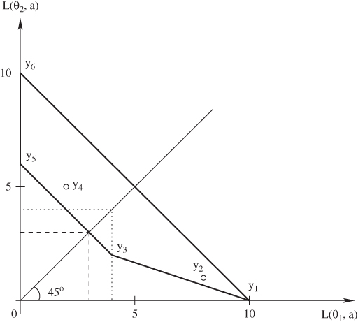
Figure 7.2 Losses and minimax action. The minimax action is a₃, represented by point y₃. The minimax randomized action is to select action a₃ with probability 3/4 and action a₅ with probability 1/4.

7.2 Data-based decisions

7.2.1 Risk

From a statistical viewpoint, the interesting questions arise when the outcome of an experiment whose distribution depends on the parameter θ is available. To establish notation, let x denote the experimental outcome with possible values in the set X, and f (x|θ) is the probability density function (or probability mass, for discrete random variables). This is also called the likelihood function when seen as a function of θ. The question is: how should one use the data to make an optimal decision? To explore this question, we define a decision function (or decision rule) to be any function δ(x) with domain X and range in A. A decision function is a recipe for turning data into actions. We denote the class of all decision rules by D. The minimax and Bayes principles provide alternative approaches to evaluating decision rules.

A comment about notation: we use x and θ to denote both the random variables and their realized values. To keep things straight when computing expectations, we use E_x[g(x, θ)] to denote the expectation of the function g with respect to the marginal distribution of x, E_x|θ[g(x, θ)] for the expectation of g with respect to f (x|θ), and E_θ[g(x, θ)] for the expectation of g with respect to the prior on θ.

Wald’s original theory is based on the expected performance of a decision rule prior to the observation of the experiment, measured by the so-called risk function.

Definition 7.3 (Risk function) The risk function of a decision rule δ is

The risk function was introduced by Wald to unify existing approaches for the evaluation statistical procedures from a frequentist standpoint. It focuses on the long-term performance of a decision rule in a series of repetitions of the decision problems. Some of the industrial applications that were motivating Wald have this flavor: the Statistician crafts rules that are applied routinely as part of the production process, and are evaluated based on average performance.

7.2.2 Optimality principles

To define the minimax and expected utility principles in terms of decision rules consider the parallel between the risk R(θ, δ) and the loss L(θ, a). Just as L can be used to choose among actions, R can be used to choose among decision functions. Definitions 7.1 and 7.2 can be restated in terms of risk. For minimax:

Definition 7.4 (Minimax decision rule) A decision rule δ^M is minimax if

To define the Bayes rule we first establish a notation for the Bayes risk:

Definition 7.5 (Bayes risk) The Bayes risk associated with prior distribution π and decision strategy δ is

The Bayes rules minimize the Bayes risk, that is:

Definition 7.6 (Bayes decision rule) A decision rule δ* is Bayes with respect to π if

What is the relationship between the Bayes rule and the expected utility principle? There is a simple and intuitive way to determine a Bayes strategy, which will also clarify this question. For every x, use the Bayes rule to determine the posterior distribution of the states of the world

where

This will summarize what is known about the state of the world given the experimental outcome. Then, just as in Definition 7.2, find the Bayes action by computing the expected loss. The difference now is that the relevant distribution for computing the expectation will not be the prior π(θ) but the posterior π(θ|x) and the function to be minimized will be the posterior expected loss

This is a legitimate step as long as we accept that static conditional probability also constrain one’s opinion dynamically, once the outcome is observed (see also Chapters 2 and 3). The action that minimizes the posterior expected loss will depend on x. So, in the end, this procedure implicitly defines a decision rule, called the formal Bayes rule.

Does the formal Bayes rule satisfy Definition 7.6? Consider the relationship between the posterior expected loss and the Bayes risk:

assuming we can reverse the order of the integrals. The quantity in square brackets is the posterior expected loss. Our intuitive recipe for finding a Bayes strategy was to minimize the posterior expected loss for every x. But in doing this we inevitably minimize r as well, and this satisfies Definition 7.6. Conversely, if we wish to minimize r with respect to the function δ, we must do so pointwise in x, by minimizing the integral in square brackets.

The conditions for interchangeability of integrals are not to be taken for granted. See Problem 8.7 for an example. Another important point is that the formal Bayes rule may not be unique, and there are examples of nonunique formal Bayes rules whose risk functions differ. More about this in Chapter 8—see for example worked Problem 8.1.

7.2.3 Rationality principles and the Likelihood Principle

The use of formal Bayes rules is backed directly by the axiomatic theory, and has profound implications for statistical inference. First, for a given experimental outcome x, a Bayes rule can be determined without any averaging over the set of all possible alternative experimental outcomes. Only the probabilities of the observed outcome under the various possible states of the world are relevant. Second, all features of the experiment that are not captured in f(x|θ) do not enter the calculation of the posterior expected loss, and thus are also irrelevant for the statistical decision. The result is actually stronger: f(x|θ) can be multiplied by an arbitrary nonzero function of x without altering the Bayes rule. Thus, for example, the data can be reduced by sufficiency, as can be seen by plugging the factorization theorem (details in Section 8.4.2) into the integrals above. This applies to both the execution of a decision once data are observed and the calculation of the criterion that is used for choosing between rules.

That all of the information in x about θ is contained in the likelihood function is a corollary of the expected utility paradigm, but is so compelling that it is taken by some as an independent principle of statistical inference, under the name of the Likelihood Principle. This is a controversial principle because the majority of frequentist measures of evidence, including highly prevalent ones such as coverage probabilities, and p-values, violate it. A monograph by Berger and Wolpert (1988) elaborates on this theme, and includes extensive and insightful discussions by several other authors as well. We will return to the Likelihood Principle in relation to optional stopping in Section 15.6.

Example 7.1 While decision rules derived from the expected utility principle satisfy the Likelihood Principle automatically, the same is not true of minimax rules. To illustrate this point in a simple example, return to the loss function in Table 7.1 and consider the regret form. In the absence of data, the minimax action is a₁. Now, suppose you can observe a binary variable x, and you can do so under two alternative experimental designs with sampling distributions f¹ and f², shown in Table 7.3. Because there are two possible outcomes and two possible actions, there are four possible decision functions:

In the sampling models of Table 7.3 we have f²(x = 1|θ) = 3f¹(x = 1|θ) for all θ ∊ Θ; that is, if x = 1 is observed, the two likelihood functions are proportional to each other. This implies that when x = 1 the expected utility rule will be the same under either sampling model. Does the same apply to minimax? Let us consider the risk functions for the four decision rules shown in Table 7.4. Under f¹ the minimax decision rule is . However, under f² the minimax decision rule is . Thus, if we observe x = 1 under f¹, the minimax decision is a₂, while under f² it is a₁. This is a violation of the Likelihood Principle.

Table 7.3 Probability functions for two alternative sampling models.

	θ1	θ2	θ3
f1(x = 1|θ)	0.20	0.10	0.25
f2(x = 1|θ)	0.60	0.30	0.75

For a concrete example, imagine measuring an ordinal outcome y with categories 0, 1/3, 2/3, 1, with likelihood as in Table 7.5. Rather than asking about y directly we can use two possible questionnaires giving dichotomous answers x. One, corresponding to f¹, dichotomizes y into 1 versus all else, while the other, corresponding to f², dichotomizes y into 0 versus all else. Because categories 1/3, 2/3, 1 have the same likelihood, f² is the better instrument overall. However, if the answer is x = 1, then it does not matter which instrument is used, because in both cases we know that the underlying latent variable must be either 1 or a value which is equivalent to it as far as learning about θ is concerned. The fact that in a different experiment the outcome could have been ambiguous about y in one dichotomization and not in the other is not relevant according to the Likelihood Principle. However, the risk function R, which depends on the whole sampling distribution, and is concerned about long-run average performance of the rule over repeated experiments, is affected. A couple of famous examples of standard inferential approaches that violate the Likelihood Principle in somewhat embarrassing ways are in Problems 7.12 and 8.5.

Table 7.4 Risk functions for the four decision rules, under the two alternative sampling models of Table 7.3.

	Under f1(.|θ)			Under f2(.|θ)
	θ1	θ2	θ3	θ1	θ2	θ3
δ1(x)	0.00	0.00	1.00	0.00	0.00	1.00
δ2(x)	2.00	4.00	0.00	2.00	4.00	0.00
δ3(x)	1.60	3.60	0.25	0.80	2.80	0.75
δ4(x)	0.40	0.40	0.75	1.20	1.20	0.25

Table 7.5 Probability functions for the unobserved outcome y underlying the two sampling models of Table 7.3.

	θ1	θ2	θ3
f(y = 1|θ)	0.20	0.10	0.25
f(y = 2/3|θ)	0.20	0.10	0.25
f(y = 1/3|θ)	0.20	0.10	0.25
f(y = 0|θ)	0.40	0.70	0.25

7.2.4 Nuisance parameters

The realistic specification of a sampling model often requires parameters other than those of primary interest. These additional parameters are called “nuisance parameters.” This is one of the very few reasonably named concepts in statistics, as it causes all kinds of trouble to frequentist and likelihood theories alike. Basu (1975) gives a critical discussion.

From a decision-theoretic standpoint, we can think of nuisance parameters as those which appear in the sampling distribution, but not in the loss function. We formalize this notion from a decision-theoretic viewpoint and establish a general result for dealing with nuisance parameters in statistics. The bottom line is that the expected utility principle justifies averaging the likelihood and the prior over the possible values of the nuisance parameter and taking things from there. In probabilistic terminology, nuisance parameters can be integrated out, and the original decision problem can be replaced by its marginal version. More specifically:

Theorem 7.1 If θ can be partitioned into (θ*, η) such that the loss L(θ, a) depends on θ only through θ*, then η is a nuisance parameter and the Bayes rule for the problem with likelihood f(x|θ) and prior π(θ) is the same as the Bayes rule for the problem with likelihood

and prior

where H is the domain of η.

Proof: We assume that all integrals involved are finite. Take any decision rule δ. The Bayes risk is

that is the Bayes risk for the problem with likelihood f*(x|θ*) and prior π(θ*). We used the independence of L on η, and the relation π(θ) = π(η, θ*) = π(η|θ*)π(θ*).

This theorem puts to rest the issue of nuisance parameters in every conceivable statistical problem, as long as one can specify reasonable priors, and compute integrals. Neither is easy, of course. Priors on high-dimensional nuisance parameters can be very difficult to assess based on expert knowledge and often include surprises in the form of difficult-to-anticipate implications when nuisance parameters are integrated out. Integration in high dimension has made much progress over the last 20 years, thanks mostly to Markov chain Monte Carlo (MCMC) methods (Robert & Casella 1999), but is still hard, in part because we tend to adapt to this progress and specify models that are at the limit of what is computable. Nonetheless, the elegance and generality of the solution are compelling.

Another way to interpret the Bayesian solution to the nuisance parameter problem is to look at posterior expected losses. An argument similar to that used in the proof of Theorem 7.1 would show that one can equivalently compute the posterior expected losses based on the marginal posterior distribution of θ* given by

This highlights the fact that the Bayes rule is potentially affected by any of the features of the posterior distribution π(η|x) of the nuisance parameter, including all aspects of the uncertainty that remains about them after observing the data. This is in contrast to approaches that eliminate nuisance parameters by “plugging in” best estimates either in the likelihood function or in the decision rule itself. The empirical Bayes approach of Section 9.2.2 is an example.

7.3 The travel insurance example

In this section we introduce a mildly realistic medical example that will hopefully afford the simplest possible illustration of the concepts introduced in this chapter and also give us the excuse to introduce some terminology and graphics from decision analysis. We will return to this example when we consider multistage decision problems in Chapters 12 and 13.

Suppose that you are from the United States and are about to take a trip overseas. You are not sure about the status of your vaccination against a certain mild disease that is common in the country you plan to visit, and need to decide whether to buy medical insurance for the trip. We will assume that you will be exposed to the disease, but you are uncertain about whether your present immunization will work. Based on aggregate data on western tourists, the chance of developing the disease during the trip is about 3% overall. Treatment and hospital abroad would normally cost you, say, 1000 dollars. There is also a definite loss in quality of life in going all the way to an exotic country and being grounded at a local hospital instead of making the most out of your experience, but we are going to ignore this aspect here. On the other hand, if you buy a travel insurance plan, which you can do for 50 dollars, all your expenses will be covered. This is a classical gamble versus sure outcome situation. Table 7.6 summarizes the loss function for this problem.

For later reference we are going to represent this simple case using a decision tree. In a decision tree, a square denotes a decision node or decision point. The decision maker has to decide among actions, represented by branches stemming out from the decision node. A circle represents a chance node or chance point. Each branch out of the circle represents, in this case, a state of nature, though circles could also be used for experimental results. On the right side of the decision tree we have the consequences. Figure 7.3 shows the decision tree for our problem.

In a Bayesian mode, you use the expected losses to evaluate the two actions, as follows:

No insurance:	Expected loss = 1000 × 0.03 + 0 × 0.97 = 30
Insurance:	Expected loss = 50 × 0.03 + 50 × 0.97 = 50.

Table 7.6 Monetary losses associated with buying and with not buying travel insurance for the trip.

Actions	Events
	θ1: ill	θ2: not ill
Insurance	50	50
No insurance	1000	0

Figure 7.3 Decision tree for the travel insurance example. This is a single-stage tree, because it includes only one decision node along any given path.

Figure 7.4 Solved decision tree for the medical insurance example. At the top of each chance node we have the expected loss, while at the top of the decision node we have the minimum expected loss. Alongside the branches stemming out from the chance node we have the probabilities of the states of nature. The action that is not optimal is crossed out by a double line.

The Bayes decision is the decision that minimizes the expected loss—in this case not to buy the insurance. However, if the chance of developing the disease was 5% or greater, the best decision would be to buy the insurance. The solution to this decision problem is represented in Figure 7.4.

You can improve your decision making by gathering data on how likely you are to get the disease. Imagine you have the option of undergoing a medical test that informs you about whether your immunization is likely to work. The test has only two possible verdicts. One indicates that you are prone to the disease and the other indicates that you are not. Sticking with the time-honored medical tradition of calling “positive” the results of tests that suggest the presence of the most devastating illnesses, we will call positive the outcome indicating that you are disease prone. Unfortunately, the test is not perfectly accurate. Let us assume that, after some clinical experiments, it was determined that the probability that the test is positive when you really are going to get the disease is 0.9, while the probability that the test is negative when you are not going to get the disease is 0.77. For a perfect test, these numbers would be both 1. In medical terminology, the first probability represents the sensitivity of the test, while the second one represents the specificity of the test. Call x the indicator variable for the event, “The test is positive.” In the notation of this chapter, the probabilities available so far are

π(θ1) =	0.03
f(x = 1|θ1) =	0.90
f(x = 0|θ2) =	0.77.

After the test, your individual chances of illness will be different from the overall 3%. The test could provide valuable information and potentially alter your chosen course of action. The question of this chapter is precisely how to use the results of the test to make a better decision. The test seems reliable enough that we may want to buy the insurance if the test is positive and not otherwise. Is this right?

To answer this question, we will consider decision rules. In our example there are two possible experimental outcomes and two possible actions so there are a total of four possible decisions rules. These are

Decision rules δ₀ and δ₃ choose the same action irrespective of the outcome of the test: they are constant functions. Decision rule δ₁ does what comes naturally: buy the insurance only if the test indicates that you are disease prone. Decision rule δ₂ does exactly the opposite. As you might expect, it will not turn out to be very competitive.

Let us now look at the losses associated with each decision rule ignoring, for now, any costs associated with testing. Of course, the loss for rules δ₁ and δ₂ now depends on the data. We can summarize the situation as shown in Table 7.7.

Two unknowns will affect how good our choice will turn out to be: the test result and whether you will be ill during the trip. As in equation (7.14) we can choose the Bayes rule by averaging out both, beginning with averaging losses by state, and then further averaging the results to obtain overall average losses. The results are shown in Table 7.8. To illustrate how entries are calculated, consider δ₁. The average risk if θ = θ₁ is

1000 f(x = 0|θ₁) + 50 f(x = 1|θ₁) = 1000 × 0.10 + 50 × 0.90 = 145.0

while the average risk if θ = θ₂ is

0 f(x = 0|θ₂) + 50 f(x = 1|θ₂) = 0 × 0.77 + 50 × 0.23 = 11.5,

Table 7.7 Loss table for the decision rules in the travel insurance example.

	θ1: ill		θ2: not ill
	x = 0	x = 1	x = 0	x = 1
δ0(x)	$1000	$1000	$0	$0
δ1(x)	$1000	$50	$0	$50
δ2(x)	$50	$1000	$50	$0
δ3(x)	$50	$50	$50	$50

Table 7.8 Average losses by state and overall for the decision rules in the travel insurance example.

	Average losses by state		Average losses overall
	θ1: ill	θ2: not ill
δ0(x)	$1000.0	$0.0	$30.0
δ1(x)	$145.0	$11.5	$15.5
δ2(x)	$905.0	$38.5	$64.5
δ3(x)	$50.0	$50.0	$50.0

so that the overall average is

145.0 × π(θ₁) + 11.5 × π(θ₂) = 15.5 = 145.0 × 0.03 + 11.5 × 0.97 = 15.5.

Strategy δ₁(x) is the Bayes strategy as it minimizes the overall expected loss. This calculation is effectively considering the losses in Table 7.7 and computing the expectation of each row with respect to the joint distribution of θ and x. In this sense it is consistent with preferences expressed prior to observing x. You are bound to stick to the optimal rule after you actually observe x only if you also agree with the before/after axiom of Section 5.2.3. Then, an alternative derivation of the Bayes rule could have been worked out directly by computing posterior expected losses given x = 1 and x = 0, as we know from Section 7.2.2 and equation (7.15).

So far, in solving the decision problem we utilized the Bayes principle. Alternatively, if you follow the minimax principle, your goal is avoiding the largest possible loss. Let us start with the case in which no data are available. In our example, the larges loss is 50 dollars if you buy the insurance and 1000 if you do not. By this principle you should buy the medical insurance. In fact, as we examine Table 7.6, we note that the greatest loss is associated with event θ₁ no matter what the action is. Therefore the maximization step in the minimax calculation will resolve the uncertainty about θ by assuming, pessimistically, that you will become ill, no matter how much evidence you may accumulate to the contrary. To alleviate this drastic pessimism, let us express the losses in “regret” form. The argument is as follows. If you condition on getting ill, the best you can do is a loss of $50, by buying the medical insurance. The alternative action entails a loss of $1000. When you assess the worthiness of this action, you should compare the loss to the best (smallest) loss that you could have obtained. You do indeed lose $1000, but your “regret” is only for the $950 that you could have avoided spending. Applying equation (7.2) to Table 7.6 gives Table 7.9.

When reformulating the decision problem in terms of regret, the expected losses are

No insurance:	Expected loss = 950 × 0.03 + 0 × 0.97 = 28.5
Insurance:	Expected loss = 0 × 0.03 + 50 × 0.97 = 48.5.

Table 7.9 Regret loss table for the actions in the travel insurance example.

		Event
		θ1	θ2
Decision:	insurance	$0	$50
	no insurance	$950	$0

Table 7.10 Risk table for the decision rules in the medical insurance example when using regret losses.

	Risk R(θ, δ) by state		Largest risk	Average risk r(π, δ)
	θ1	θ2
δ0(x)	$950	$0	$950	$28.5
δ1(x)	$95	$11.5	$95	$14.0
δ2(x)	$855	$38.5	$855	$63.0
δ3(x)	$0	$50	$50	$48.5

The Bayes action remains the same. The expected losses become smaller, but the expected loss of every action becomes smaller by the same amount. On the contrary, the minimax action may change, though in this example it does not. The minimax solution is still to buy the insurance.

Does the optimal minimax decision change depending on the test results? In Table 7.10 we derive the Bayes and minimax rules using the regret losses. Strategy δ₁ is the Bayes strategy as we had seen before. We also note that δ₂ is dominated by δ₁, that is it has a higher risk than δ₁ irrespective of the true state of the world. Using the minimax approach, the optimal decision is δ₃, that is it is still optimal to buy the insurance irrespective of the test result. This conclusion depends on the losses, sensitivity, and specificity, and different rules could be minimax if these parameters were changed.

This example will reappear in Chapters 12 and 13, when we will consider both the decision of whether to do the test and the decision of what to do with the information.

7.4 Randomized decision rules

In this section we briefly encounter randomized decision rules. From a frequentist viewpoint, the randomized decision rules are important because they guarantee, for example, specified error levels in the development of hypothesis testing procedures and confidence intervals. From a Bayesian viewpoint, we will see that randomized decision rules are not necessary, because they cannot improve the Bayes risk compared to nonrandomized decision rules.

Definition 7.7 (Randomized decision rule) A randomized decision rule δ^R(x,.) is, for each x, a probability distribution on A. In particular, δ^R(x, A) denotes the probability that an action in A (a subset of A) is chosen. The class of randomized decision rules is denoted by D^R.

Definition 7.8 (Loss function for a randomized decision rule) A randomized decision rule δ^R(x,.) has loss

We note that a nonrandomized decision rule is a special case of a randomized decision rule which assigns, for any given x, a specific action with probability one.

In the simple setting of Figure 7.1, no randomized decision rule in D^R can improve the Bayes risk attained with a nonrandomized Bayes decision rule in D. This turns out to be the case in general:

Theorem 7.2 For every prior distribution π on Θ, the Bayes risk on the set of randomized estimators is the same as the Bayes risk on the set of nonrandomized estimators, that is

For a proof see Robert (1994). This result continues to hold when the Bayes risk is not finite, but does not hold if r is replaced by R(θ, δ) unless additional conditions are imposed on the loss function (Berger 1985).

DeGroot comments on the use of randomized decision rules:

The next three sections illustrate these concepts in common statistical decision problems: classification, hypothesis testing, point and interval estimation.

7.5 Classification and hypothesis tests

7.5.1 Hypothesis testing

Contrasting their approach to Fisher’s significance testing, Neyman and Pearson write:

This insight was one of the foundations of Wald’s work, so hypothesis tests are a natural place to start visiting some examples. In statistical decision theory, hypothesis testing is typically modeled as the choice between actions a₀ and a₁, where a_i denotes accepting hypothesis H_i: θ ∊ Θ_i, with i either 0 or 1. Thus, A = {a₀, a₁} and Θ = Θ₀ ∪ Θ₁. A discussion of what it really means to accept a hypothesis could take us far astray, but is not a point to be taken lightly. An engaging reading on this subject is the debate between Fisher and Neyman about the meaning of hypothesis tests, which you can track down from Fienberg (1992).

If the hypothesis test is connected to a concrete problem, it may be possible to specify a loss function that quantifies how to penalize the consequences of choosing decision a₀ when H₁ is true, and decision a₁ when H₀ is true. In the simplest formulation it only matters whether the correct hypothesis is accepted, and errors are independent of the variation of the parameter θ within the two hypotheses. This is realistic, for example, when the practical consequences of the decision depend primarily on the direction of an effect. Formally,

Here L₀ and L₁ are positive numbers and I_A is the indicator of the event A. Table 7.11 restates the same assumption in a more familiar form.

Table 7.11 A simple loss function for the hypothesis testing problem.

	θ ∊ Θ0	θ ∊ Θ1
a0	0	L0
a1	L1	0

As the decision space is binary, any decision rule δ must split the set of possible experimental results into two sets: one associated with a₀ and the other with a₁. The risk function is

From the point of view of finding optima, losses can be rescaled arbitrarily, so any solution, minimax or Bayes, will only depend on L₁ and L₀ through their ratio.

If the sets Θ₀ and Θ₁ are singletons (the familiar simple versus simple hypotheses test) we can, similarly to Figures 7.1 and 7.2, represent any decision rule as a point in the space R(θ₀, δ), R(θ₁, δ), called the risk space. The Bayes and minimax optima can be derived using the same geometric intuition based on lines and wedges. If the data are from a continuous distribution, the lower solid line of Figures 7.1 and 7.2 will often be replaced by a smooth convex curve, and the solutions will be unique. With discrete data there may be a need to randomize to improve minimax solutions.

We will use the terms null hypothesis for H₀ and alternative hypothesis for H₁ even though the values of L₀ and L₁ are the only real element of differentiation here. In this terminology, α_δ and β_δ can be recognized as the probabilities of type I and II errors. In the classical Neyman–Pearson hypothesis testing framework, rather than specifying L₀ and L₁ one sets the value for sup_{θ∊Θ0} α_δ(θ) and minimizes β_δ(θ), θ ∊ Θ₁, with respect to δ. Because β_δ(θ) is one minus the power, a uniformly most powerful decision rule will have to dominate all others in the set Θ₁. For a comprehensive discussion on classical hypothesis testing see Lehmann (1997).

In the simple versus simple case, it is often possible to set L₁/L₀ so that the minimax approach and Neyman–Pearson approach for a fixed α lead to the same rule. The specification of α and that of L₁/L₀ can substitute for each other. In all fields of science, the use of α = 0.05 is often taken for granted, without any serious thought being given to the implicit balance of losses. This has far-reaching negative consequences in both science and policy.

Moving to the Bayesian approach, we begin by specifying a prior π on θ. Before making any observation, the expected losses are

Thus, the Bayes action is a₀ if

and otherwise it is a₁. In particular, if L₀ = L₁, the Bayes action is a₀ whenever π(θ ∊ Θ₀) > 1/2. By a similar argument, after data are available, the function

is the posterior expected loss and the formal Bayes rule is to choose a₀ if

and otherwise to choose a₁. The ratio of posterior probabilities on the right hand side can be written as

where

for i = 0, 1. The ratio of posterior probabilities can be further expanded as

that is, a product of the prior odds ratio and the so-called Bayes factor BF = f(x|θ ∊ Θ₀)/f(x|θ ∊ Θ₁). The decision depends on the data only through the Bayes factor. In the definition above we follow Jeffreys’ definition (Jeffreys 1961) and place the null hypothesis in the numerator, but you may find variation in the literature. Bernardo and Smith (1994) provide further details on the Bayes factors in decision theory.

The Bayes factor has also been proposed by Harold Jeffreys and others as a direct and intuitive measure of evidence to be used in alternative to, say, p-values for quantifying the evidence against a hypothesis. See Kass and Raftery (1995) and Goodman (1999) for recent discussions of this perspective. Jeffreys (1961, Appendix B) proposed the rule of thumb in Table 7.12 to help with the interpretation of the Bayes factor outside of a decision context. You can be the judge of whether this is fruitful — in any case, the contrast between this approach and the explicit consideration of consequences is striking.

Table 7.12 Interpretation of the Bayes factors for comparison between two hypotheses, according to Jeffreys.

Grade	2 log10 BF	Evidence
0	≥ 0	Null hypothesis supported
1	–1/2 to 0	Evidence against H0, but not worth more than a bare mention
2	–1 to –1/2	Evidence against H0 substantial
3	–3/2 to –1	Evidence against H0 strong
4	–2 to –3/2	Evidence against H0 very strong
5	<–2	Evidence against H0 decisive

The Bayes decision rule presented here is broadly applicable beyond a binary partition of the parameter space. For example, it extends easily to nuisance parameters, and can be applied to any pair of hypotheses selected from a discrete set, as we will see in the context of model choice in Section 11.1.2. One case that requires a separate and more complicated discussion is the comparison of a point null with a composite alternative (see Problem 7.3).

7.5.2 Multiple hypothesis testing

A trickier breed of decision problems appears when we wish to jointly test a battery of related hypotheses all at once. For example, in a clinical trial with four treatments, there are six pairwise comparisons we may be interested in. At the opposite extreme, a genome-wide scan for genetic variants associated with a disease may give us the opportunity to test millions of associations between genetic variables and a disease of interest (Hirschhorn and Daly 2005). In this section we illustrate a Bayesian decision-theoretic approach based on Müller et al. (2005). We will not venture here into the frequentist side of multiple testing. A good entry point is Hochberg and Tamhane (1987). Some considerations contrasting the two approaches are in Berry and Hochberg (1999), Genovese and Wasserman (2003), and Müller et al. (2007b).

The setting is this. We are interested in I null hypotheses θ_i = 0, with i = 1, ..., I, to be compared against the corresponding alternatives θ_i = 1. Available decisions for each i are a rejection of the null hypotheses (a_i = 1), or not (a_i = 0). In massive comparison problems, rejections are sometimes called discoveries, or selections. I-dimensional vectors θ and a line up all the hypotheses and corresponding decisions. The set of indexes such as a_i = 1 is a list of discoveries. In many applications, list making is a good way to think about the essence of the problem. To guide us in the selection of a list we observe data x with distribution f(x|θ, η), where η gathers any remaining model parameters. A key quantity is π_x(θ_i = 1), the marginal posterior probability that the ith null hypothesis is false. The nuisance parameters η can be removed by marginalization at the start, as we saw in Section 7.2.4.

The choice of a specific loss function is complicated by the fact that the experiment involves two competing goals, discovering as many as possible of the components that have θ_i = 1, while at the same time controlling the number of false discoveries. We discuss two alternative utility functions that combine the two goals. These capture, at least as a first approximation, the goals of massive multiple comparisons, are easy to evaluate, lead to simple decision rules, and can be interpreted as generalizations of frequentist error rates. Interestingly, all will lead to terminal decision rules of the same form. Other loss functions for multiple comparisons are discussed in the seminal work of Duncan (1965).

We start with the notation for the summaries that formalize the two competing goals of controlling false negative and false positive decisions. The realized counts of false discoveries and false negatives are

Writing D = ∑ a_i for the number of discoveries, the realized percentages of wrong decisions in each of the two lists, or false discovery rate and false negative rate, are, respectively

FD(·), FN(·), FDR(·), and FNR(·) are all unknown. The additional term ε avoids a zero denominator.

We consider two ways of combining the goals of minimizing false discoveries and false negatives. The first two specifications combine false negative and false discovery rates and numbers, leading to the following loss functions:

The loss function L_N is a natural extension of the loss function of Table 7.11 with k = L₁/L₀. From this perspective the combination of error rates in L_R seems less attractive, because the losses for a false discovery and a false negative depend on the total number of discoveries or negatives, respectively.

Alternatively, we can model the trade-offs between false negatives and false positives as a multicriteria decision. For the purpose of this discussion you can think of multicriteria decisions as decisions in which the loss function is multidimensional. We have not seen any axiomatic foundation for this approach, which you can learn about in Keeney et al. (1976). However, the standard approach to selecting an action in multicriteria decision problems is to minimize one dimension of the expected loss while enforcing a constraint on the remaining dimensions. The Neyman–Pearson approach to maximizing power subject to a fixed type I error, seen in Section 7.5.1, is an example. We will call L_2N and L_2R the multicriteria counterparts of L_N and L_R.

Conditioning on x and marginalizing with respect to θ, we obtain the posterior expected FD and FN

and the corresponding and . See also Genovese and Wasserman (2002). Using these quantities we can compute posterior expected losses for both loss formulations, and also define the optimal decisions under L_2N as minimization of subject to . Similarly, under L_2R we minimize subject to .

Under all four loss functions the optimal decision about the multiple comparison is to select the dimensions that have a sufficiently high posterior probability π(θ_i = 1|x), using the same threshold for all dimensions:

Theorem 7.3 Under all four loss functions the optimal decision takes the form

a(t*) defined as a_i = 1 if and only if π(θ_i = 1|x) ≥ t*.

The optimal choices of t* are

In the expression for , v_(i) is the ith order statistic of the vector {π(θ₁ = 1|x), ..., π(θ_n = 1|x)}, and D* is the optimal number of discoveries.

The proof is in the appendix of Müller et al. (2005).

Under L_R, L_2N, and L_2R the optimal threshold t* depends on the observed data. The nature of the terminal decision rule a_i is the same as in Genovese and Wasserman (2002), who discuss a more general rule, allowing the decision to be determined by cutoffs on any univariate summary statistic.

A very early incarnation of this result is in Pitman (1965) who considers, from a frequentist standpoint, the case where one wishes to test I simple hypotheses versus the corresponding simple alternatives. The experiments and the hypotheses have no connection with each other. If the goal is to maximize the average power, subject to a constraint on the average type I error, the optimal solution is a likelihood ratio test for each hypothesis, and the same cutoff point is used in each.

7.5.3 Classification

Binary classification problems (Duda et al. 2000) consider assigning cases to one of two classes, based on measuring a series of attributes of the cases. An example is medical diagnosis. In the simplest formulation, the action space has two elements: “diagnosis of disease” (a₁) and “diagnosis of no disease” (a₀). The states of “nature” (the patient, really) are disease or no disease. The loss function, shown in Table 7.13, is the same we used for hypothesis testing, with L₀ representing the loss of diagnosing a diseased patient as healthy, and L₁ representing the loss of diagnosing a healthy patient as diseased.

The main difference here is that we observe data on the attributes x and correct disease classification y of a sample of individuals, and wish to classify an additional individual, randomly drawn from the same population. The model specifies f(y_i|x_i, θ) for individual i. If are the observed features of the new individual to be classified, and is the unknown disease state, the ingredients for computing the posterior predicted probabilities are

where M is the marginal probability of (x,y). From steps similar to Section 7.5.1, the Bayes rule is to choose a diagnosis of no disease if

This classification rule incorporates inference on the population model, uncertainty about population parameters, and relative disutilities of misclassification errors.

Table 7.13 A loss function for the binary classification problem.

	No disease	Disease
a0	0	L0
a1	L1	0

7.6 Estimation

7.6.1 Point estimation

Statistical point estimation assigns a single best guess to an unknown parameter. This assignment can be viewed as a decision problem in which A = Θ. Decision functions map data into point estimates, and they are also called estimators. Even though point estimation is becoming a bit outdated because of the ease of looking at entire distributions of unknowns, it is an interesting simplified setting for examining the implications of various decision principles.

In this setting, the loss function measures the error from declaring that the estimate is a when the correct value is θ. Suppose that A = Θ = ℜ and that the loss function is quadratic, L(θ, a) = (θ – a)². This loss has been a long-time favorite because it leads to easily interpretable analytic results. In fact its use goes back at least as far as Gauss. With quadratic loss, the risk function can be broken down into two pieces as

The first term in the decomposition is the variance of the decision rule and the second term is its bias, squared.

Another interesting fact is that the Bayes rule is simply δ*(x) = E[θ|x], that is the posterior mean. This is because the posterior expected loss is

which is minimized by taking a* = E[θ|x]. Thus, the posterior expected loss associated with a* is the posterior variance of θ. If instead L(θ, a) = |θ – a|, then δ*(x) = median of π(θ|x).

A widely accepted estimation paradigm is that of maximum likelihood (Fisher 1925). The decision-theoretic framework is useful in bringing out the implicit value system of the maximum likelihood approach. To illustrate, take a discrete parameter space Θ = {θ₁, θ₂, ...} and imagine that the estimation problem is such that we gain something only if our estimate is exactly right. The corresponding loss function is

L(θ, a) = I_{a≠θ},

where, again, a represents a point estimate of θ. The posterior expected loss is maximized by a* = mode(θ|x) ≡ θ⁰ (use your favorite tie-breaking rule if there is more than one mode). If the prior is uniform on Θ (and in other cases as well), the mode of the posterior distribution will coincide with the value of θ that maximizes the likelihood.

Extending this correspondence to the continuous case is more challenging, because the posterior probability of getting the answer exactly right is zero. If we set

L(θ, a) = I_{{|a−θ|≥ε}},

then the Bayes rule is the value of a that has the largest posterior mass in a neighborhood of size ε. If the posterior is a density, and the prior is approximately flat, then this a will be close to the value maximizing the likelihood.

In the remainder of this section we present two simple illustrations.

Example 7.2 This example goes back to the “secret number” example of Section 1.1. You have to guess a secret number. You know it is an integer. You can perform an experiment that would yield either the number before it or the number after it, with equal probability. You know there is no ambiguity about the experimental result or about the experimental answer. You can perform the experiment twice. More formally, x₁ and x₂ are independent observations from

where Θ are the integers. We are interested in estimating θ using the loss function L(θ, a) = I_{{a ≠ θ}}. The estimator

is equal to θ if and only if x₁ ≠ x₂, which happens in one-half of the samples. Therefore R(θ, δ₀) = 1/2. Also the estimator

δ₁(x₁, x₂) = x₁ + 1

is equal to θ if x₁ < θ, which also happens in one-half of the samples. So R(θ, δ₁) = 1/2. These two estimators are indistinguishable from the point of view of frequentist risk.

What is the Bayes strategy? If x₁ ≠ x₂ then

and the optimal action is a* = (x₁ + x₂)/2. If x₁ = x₂, then

and similarly,

so that the optimal action is x₁ + 1if π(x₁ + 1) ≥ π(x₁ – 1) and x₁ – 1if π(x₁ + 1) ≤ π(x₁ – 1). If the prior is such that it is approximately Bayes to choose x₁ + 1 if x₁ = x₂, then the resulting Bayes rule has frequentist risk of 1/4.

Example 7.3 Suppose that x is drawn from a N(θ, σ²) distribution with σ² known. Let L(θ, a) = (θ – a)² be the loss function. We want to study properties of rules of the form δ(x) = cx, for c a real constant. The risk function is

R(θ, δ)	= Var[cx|θ] + [E[cx|θ] – θ]2
	= c2σ2 + (c – 1)2θ2.

First off we can rule out a whole bunch of rules in the family. For example, as illustrated in Figure 7.5, all the δ with c > 1 are dominated by the c = 1 rule, because R(θ, x) < R(θ, cx), ∀ θ. So it would be foolish to choose c > 1. In Chapter 8 we will introduce technical terminology for this kind of foolishness. The rule δ(x) = x is a bit special. It is unbiased and, unlike the others, has the same risk no matter what θ is. This makes it the unique minimax rule in the class, because all others have a maximum risk of infinity. Rules with 0 < c < 1, however, are not dominated by δ(x) = x, because they have a smaller variance, which may offset the higher bias when θ is indeed small.

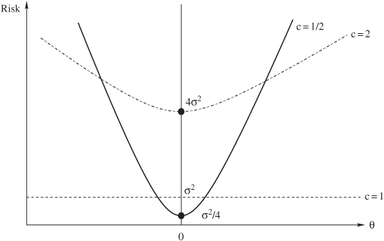
Figure 7.5 Risk functions for c = 1/2, 1, and 2. The c = 2 rule is dominated by the c = 1 rule, while no dominance relation exists between the c = 1/2 and c = 1 rules.

One way of understanding why one may want to use a c that is not 1 is to bring in prior information. For example, say , where μ₀ and are known. After x is observed, the posterior expected loss is the posterior variance and the Bayes action is the posterior mean. Thus, using the results from Chapter 16,

When μ₀ = 0 the decision rule belongs to the family we are studying for . To see what happens when μ₀ ≠ 0 study the class δ(x) = c₀ + cx.

7.6.2 Interval inference

A common practice in statistical analysis is to report interval estimates, to communicate succinctly both the likely magnitude of an unknown and the uncertainty remaining after analysis. Interval estimation can also be framed as a decision problem, in fact Wald was doing so as early as 1939. Rice et al. (2008) review decision-theoretic approaches to interval estimation and Schervish (1995) provides a through treatment. Rice et al. (2008) observe that loss functions for intervals should trade off two competing goals: intervals should be small and close to the true value. One of the illustrations they provide is this. If Θ is the parameter space, we need to choose an interval a = (a₁, a₂) within that space. A loss function capturing the two competing goals of size and closeness is a weighted combination of the half distance between the points and the “miss-distance,” that is zero if the parameter is in the interval, and is the distance between the parameter and the nearest extreme if the parameter is outside the interval:

Here the subscript + indicates the positive part of the corresponding function: g₊ is g when g is positive and 0 otherwise. If this loss function is used, then the optimal interval is to choose a₁ and a₂ to be the L₁/(2L₂) and 1 – L₁/(2L₂) quantiles of the posterior distribution of θ. This provides a decision-theoretic justification for the common practice of computing equal tail posterior probability regions. The tail probability is controlled by the parameters representing the relative importance of size versus closeness. Analogously to the hypothesis test case, the same result can be achieved by specifying L₁/L₂ or the probability α assigned to the two tails in total.

An alternative specification of the loss function leads to a solution based on moments. This loss is a weighted combination of the half distance between the points and the distance of the true parameter from the center of the interval. This is measured as squared error, standardized to the interval’s half size:

The Bayes interval in this case is

Finally, Carlin and Louis (2008) consider the loss function

L(θ, a) = I_θ∉a + c × volume(a).

Here c controls the trade-off between the volume of a and the posterior coverage probability. Under this loss function, the Bayes rule is the subset of Θ including values with highest posterior density, or HPD region(s).

7.7 Minimax–Bayes connections

When are the Bayes rules minimax? This question has been studied intensely, partly from a game–theoretic perspective in which the prior is nature’s randomized decision rule, and the Bayes venue allows a minimax solution to be found. From a statistical perspective, the bottom line is that often one can concoct a prior distribution that is sufficiently pessimistic that the Bayes solution ends up being minimax. Conceptually this is important, because it establishes intersection between the set of all possible Bayes rules, each with its own prior, and minimax rules (which are often not unique), despite the different premises of the two approaches. Technically, matters get tricky very quickly. Our discussion is a quick tour. Much more thorough accounts are given by Schervish (1995) and Robert (1994).

The first result establishes that if a rule δ has a risk R that can be bounded by the average risk r of a Bayes rule, then it is minimax. This also applies to limits of r over sequences of priors.

Theorem 7.4 Let be the Bayes rule with respect to π_k. Suppose that . If there is δ^M such that R(θ, δ^M) ≤ c for all θ, then δ^M is minimax.

Proof: Suppose by contradiction that δ^M is not minimax. Then, there is δ′ and > 0 such that

Take k* such that

Then, for k ≥ k*,

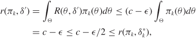
but this contradicts the hypothesis that is a Bayes rule with respect to π_k.

Example 7.4 Suppose that x₁, ..., x_p are independent and distributed as N(θ_i,1). Let x = (x₁, ..., x_p)′ and θ = (θ₁, ..., θ_p)′. We are interested in showing that the decision rule δ^M(x) = x is minimax if one uses an additive quadratic loss function

The risk function of δ^M is

To build our sequence of priors, we set prior π_k to be such that the θ are independent normals with mean 0 and variance k. With this prior and quadratic loss, the Bayes rule is given by the vector of posterior means, that is

Note that the θ_i, i = 1, ..., p, are independent a posteriori with variance k/(k + 1). Therefore, the Bayes risk of is

Taking the limit,

The assumptions of Theorem 7.4 are all met and therefore δ^M is minimax. This example will be developed in great detail in Chapter 9.

We now give a more formal definition of what it means for a prior to be pessimistic for the purpose of our discussion on minimax: it means that that prior implies the greatest possible Bayes risk.

Definition 7.9 A prior distribution π^M for θ is least favorable if

π^M is also called the maximin strategy for nature.

Theorem 7.5 Suppose that δ* is a Bayes rule with respect to π^M and such that

Then

1. δ* is a minimax rule.

2. If δ* is the unique Bayes rule with respect to π, then δ* is the unique minimax rule.

3. π^M is the least favorable prior.

Proof: To prove 1 and 2 note that

where the inequality is for any other decision rule δ, because δ* is a Bayes rule with respect to π^M. When δ^M is the unique Bayes rule a strict inequality holds. Moreover,

Thus,

and δ^M is a minimax rule. If δ* is the unique Bayes rule, the strict inequality noted above implies that δ* is the unique minimax rule.

To prove 3, take any other Bayes rule δ with respect to a prior distribution π. Then

that is π^M is the least favorable prior.

Example 7.5 Take x to be binomial with unknown θ, assume a quadratic loss function L(θ, a) = (θ – a)², and assume that θ has a priori Beta(α₀, β₀) distribution. Under quadratic loss, the Bayes rule, call it δ*, is the posterior mean

and its risk is

If , we have

This rule has constant risk

Since the risk is constant, R(θ, δ^M) = r(π^M, δ^M) for all θ, and π^M is a Beta(, ) distribution. By applying Theorem 7.5 we conclude that δ^M is minimax and π^M is least favorable.

The maximum likelihood estimator δ, under quadratic loss, has risk θ(1 – θ)/n which has a unique maximum at θ = 1/2. Figure 7.6 compares the risk of the maximum likelihood estimator δ to that of the minimax estimator δ^M for four choices of n. For small values of n, the minimax estimator is better for most values of the parameter. However, for larger values of n the improvement achieved by the minimax estimator is negligible and limited to a narrow range.

Example 7.6 We have seen how to determine minimax rules for normal and binomial data. Lehmann (1983) shows how to use these results to derive minimax estimators for the means of arbitrary distributions, under a much more general setting than the parametric assumptions considered so far. The general idea is captured in the following lemma.

Figure 7.6 Risk functions for n = 1, 10, 100, 1000 as a function of θ. In each panel, the solid line shows the risk function for the maximum likelihood estimator δ, while the dotted line shows the flat risk function for the minimax estimator δ^M.

Lemma 2 Let x be a random quantity with unknown distribution F, and let g(F) be a functional defined over a set F₁ of distributions F. Suppose that δ^M is a minimax estimator of g(F) when F is restricted to some subset F₀ of F₁. Then if

then δ^M is minimax also when F is permitted to vary over F₁.

See Lehmann (1983) for details. We will look at two examples where the functional g is the mean of F. Let x₁, ..., x_n be independent and identically distributed observations from F, and such that E[x_i|θ] = θ < ∞, for i = 1, ..., n. We consider the problem of estimating θ under quadratic loss L(θ, a) = (θ – a)².

For a real-valued observation, we impose the restriction of bounded variance of F, that is

Distributions with bounded variance will constitute our class F₁. Bounded variance will guarantee that the maximum risk of reasonable estimators of θ is finite. We choose F₀ to be the family of normal distributions for which restriction (7.25) also holds. Similarly to Example 7.4, assume that the prior distribution of θ is N(μ₀, k). Under quadratic loss the Bayes estimator is the posterior mean and the Bayes risk is the posterior variance. This gives

Now focus on . Since and R(θ, δ^M) = σ²/n, by applying Theorem 7.4 we conclude that is minimax for F₀. Using the lemma, δ^M is minimax for F₁.

Now take F₁ to be the class of distributions F such that F(1) – F(0) = 1. These distributions have bounded support, a condition which allow us to work with finite risk without bounding the variance. Let F₀ be the Bernoulli family of distributions. These are such that f(x_i = 1|θ) = θ and f(x_i = 0|θ) = 1 – θ, where 0 < θ < 1. Let us consider the estimator

As we saw in Example 7.5, δ^M is the minimax estimator of θ as F varies in F₀. To prove that δ^M is minimax with respect to F₁, by virtue of the lemma, it is enough to show that the risk R(θ, δ^M) takes on its maximum over F₀. Observe that the risk is

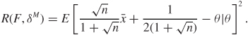
By adding and subtracting we obtain

Observe that 0 ≤ x ≤ 1. Then x² ≤ x and Var[x|θ] = E[x²|θ] – θ² ≤ E[x|θ] – θ². Therefore

As seen in Example 7.5, the quantity is the risk of δ^M over F₀. Since the risk function of δ^M takes its maximum over F₀, we can conclude that δ^M is minimax for the broader family F₁.

We close our discussion with a general sufficient condition under which minimax rules and least favorable distributions exist.

Theorem 7.6 (The minimax theorem) Suppose that the loss function L is bounded below and Θ is finite. Then

and there exists a least favorable distribution π^M. If R is closed from below, then there is a minimax rule that is a Bayes rule with respect to π^M.

See Schervish (1995) for a proof. Weiss (1992) elaborates on the significance of this result within Wald’s theory. The following example illustrates that the theorem does not necessarily hold if Θ is not finite.

Example 7.7 (Ferguson 1967) Suppose that θ = A = {1, 2, ...}, in a decision problem where no data are available and the loss function is

If we think of this as a game between the Statistician and Nature, both have to pick an integer, and whoever chooses the largest integer wins the game. Priors can formally be thought of as randomized strategies for Nature, so π(θ_i) is the probability of Nature choosing integer i. We have r(π, a) = E_θ[L(θ, a)] = P(θ > a) – P(θ < a). Therefore, sup_π inf_a r(π, a) = −1, which differs from inf_a sup_θ R(θ, a) = 1. Thus, we do not have an optimal minimax strategy for this game.

7.8 Exercises

Problem 7.1 Lindley reports this interesting gastronomical conundrum with regard to minimax:

Construct functions u, and L_u and L, that provide a numerical illustration of Lindley’s example. This paradox is induced by the transformation to regret, so you only need to go as far as illustrating the paradox for L.

Problem 7.2 You are collecting n normal observations with mean θ and standard deviation 1 because you are interested in testing θ = θ₀ = −1 versus θ = θ₁ = 1. Using the notation of Section 7.5.1:

1. Find the set of values of π, L₀, and L₁ that give you the same decision rule as the most powerful α level test, with α = 0.04.

2. Can you find values of π, L₀, and L₁ that give you the same decision rule as the most powerful α level test, with α = 0.04, for both a sample of size n and a sample of size 2n?

3. (Optional) If your answer to the second question is no, that means that using the same α irrespective of sample size violates some of the axioms of expected utility theory. Can you say which?

Problem 7.3 Testing problems are frequently cast in terms of comparisons between a point null hypothesis, that is a hypothesis made up of a single point in the parameter space, against a composite alternative, including multiple points. Formally, Θ₀ = θ₀ and Θ₁ ≠ θ₀. A standard Bayesian approach to this type of problem is to specify a mixture prior for θ that assigns a point mass π₀ to the event Θ = θ₀ and a continuous distribution π₁(θ|θ ∊ Θ₁). This is sometimes called “point and slab” prior and goes back to Jeffreys (1961). Given data x ~ f(x|θ), find the Bayes rule in this setting. Read more about this problem in Berger & Delampady (1987).

Problem 7.4 You are collecting normal data with mean θ and standard deviation 1 because you are interested in testing θ < 0 versus θ ≥ 0. Your loss is such that mistakes are penalized differently within the alternative compared to the null, that is

1. Assume a uniform prior on θ and use Bayes’ theorem to derive the posterior distribution.

2. Find the posterior expected losses of a₀ and a₁.

3. Find the Bayes decision rule for this problem.

Problem 7.5 Find the least favorable priors for the two sampling distributions in Example 7.1. Does it bother you that the prior depends on the sampling model?

Problem 7.6 In order to choose an action a based on the loss L(θ, a), you elicit the opinion of two experts about the probabilities of the various outcomes of θ (you can assume if you wish that θ is a discrete random variable). The two experts give you distributions π₁ and π₂. Suppose that the action a* is Bayes for both distributions π₁ and π₂. Is it true that a* must be Bayes for all weighted averages of π₁ and π₂; that is, for all the distributions of the form απ₁ + (1 – α)π₂, with 0 < α < 1?

Problem 7.7 Prove that the Bayes rule under absolute error loss is the posterior median. More precisely, suppose that E[|θ|] < ∞. Show that a number a* satisfies

if and only if a* is a median of the distribution of θ.

Problem 7.8 Let θ be a random variable with distribution π(θ) that is symmetric with respect to θ₀. Formally, π(θ + θ₀) = π(θ₀ – θ) for all θ ∊ R. Suppose that L is a nonnegative twice differentiable convex loss function on the real line that is symmetric around the value of 0. Also suppose that, for all values of a,

Prove that:

1. L is convex;

2. L is symmetric with respect to θ₀;

3. L is minimized at a = θ₀.

Problem 7.9 Derive an analogous equation to (7.17), using the same assumptions of Section 7.5.1, except now the sampling distribution is f(x|θ, ϕ), and the prior is π(θ, ϕ).

Problem 7.10 Consider a point estimation problem in which you observe x₁, ..., x_n as i.i.d. random variables from the Poisson distribution

Assume a squared error of estimation loss L(θ, a) = (a – θ)², and assume a prior distribution on θ given by the gamma density

1. Show that the Bayes decision rule with respect to the prior above is of the form

   

   where a > 0, b ∊ (0, 1), and . You may use the fact that the distribution of ∑_i x_i is Poisson with parameter nθ without proof.

2. Compute and graph the risk functions of δ*(x₁, ..., x_n) and that of the MLE .

3. Compute the Bayes risk of δ*(x₁, ..., x_n) and show that it is (a) decreasing in n and (b) it goes to 0 as n gets large.

4. Suppose an investigator wants to collect a sample that is large enough that the Bayes risk after the experiment is half of the Bayes risk before the experiment. Find that sample size.

Problem 7.11 Take x to be binomial with unknown θ and n = 2, and consider testing θ₀ = 1/3 versus θ₁ = 1/2. Draw the points corresponding to every possible decision rule in the risk space with coordinates R(θ₀, δ) and R(θ₁, δ). Identify minimax randomized and nonrandomized rules and the expected utility rule for prior π(θ₀) = 1/4. Identify the set of rules that are not dominated by any other rule (those are called admissible in Chapter 8).

Problem 7.12

State a probabilistic model for the situation described by Pratt, and specify a prior distribution and a loss function for the point estimation of the mean voltage. Writing code if necessary, compute the risk function R of the Bayes rule and that of your favorite frequentist rule in two scenarios: when the high-range voltmeter is available and when it is not. Does examining the risk function help you select a decision rule once the data are observed?