15
Stopping

In Chapter 14 we studied how to determine an optimal fixed sample size. In that discussion, the decision maker selects a sample size before seeing any of the data. Once the data are observed, the decision maker then makes a terminal decision, typically an inference. Here, we will consider the case in which the decision maker can make observations one at a time. At each time, the decision maker can either stop sampling (and choose a terminal decision), or continue sampling. The general technique for solving this sequential problem is dynamic programming, presented in general terms in Chapter 12.

In Section 15.1, we start with a little history of the origin of sequential sampling methods. Sequential designs were originally investigated because they can potentially reduce the expected sample size (Wald 1945). Our revisitation of Wald’s sequential stopping theory is almost entirely Bayesian and can be traced back to Arrow et al. (1949). In their paper, they address some limitations of Wald’s proof of the optimality of the sequential probability ratio test, derive a Bayesian solution, and also introduce a novel backward induction method that was the basis for dynamic programming. We illustrate the gains that can be achieved with sequential sampling using a simple example in Section 15.2. Next, we formalize the sequential framework for the optimal choice of the sample size in Sections 15.3.1, 15.3.2, and 15.3.3. In Section 15.4, we present an example of optimal stopping using the dynamic programming technique.

In Section 15.5, we discuss sequential sampling rules that do not require specifying the costs of experimentation, but rather continue experimenting until enough information about the parameters of interest is gained. An example is to sample until the posterior probability of a hypothesis of interest reaches a prespecified level. We examine the question of whether such a procedure could be used to design studies that always reach a foregone conclusion, and conclude that from a Bayesian standpoint, that is not the case. Finally, in Section 15.6 we discuss the role of stopping rules in the terminal decision, typically inferences, and connect our decision-theoretic approach to the Likelihood Principle.

Featured articles:

Wald, A. (1945). Sequential tests of statistical hypotheses, Annals of Mathematical Statistics 16: 117–186.

Arrow, K., Blackwell, D. and Girshick, M. (1949). Bayes and minimax solutions of sequential decision problems, Econometrica 17: 213–244.

Useful reference texts for this chapter are DeGroot (1970), Berger (1985), and Bernardo and Smith (2000).

15.1 Historical note

The earliest example of a sequential method in the statistical literature is, as far as we know, provided by Dodge and Romig (1929) who proposed a two-stage procedure in which the decision of whether or not to draw a second sample was based on the observations of the first sample. It was only years later that the idea of sequential analysis would be more broadly discussed. In 1943, US Navy Captain G. L. Schuyler approached the Statistical Research Group at Columbia University with the problem of determining the sample size needed for comparing two proportions. The sample size required was very large. In a letter addressed to Warren Weaver, W. Allen Wallis described Schuyler’s impressions:

W. Allen Wallis and Milton Friedman explored this idea and came up with the following conjecture:

They first approached Wolfowitz with this idea. Wolfowitz, however, did not show interest and was doubtful about the existence of a sequential procedure that would improve over the most powerful test. Next, Wallis and Friedman brought this problem to the attention of A. Wald who studied it and, in April of 1943, proposed the sequential probability ratio test. In the problem of testing a simple null versus a simple alternative Wald claimed that:

Wald’s finding was of immediate interest, as he explained:

It was only in 1945, after the reports of the Statistical Research Group were no longer classified, that Wald’s research was published. Wald followed his paper with a book published in 1947 (Wald 1947b).

In Chapter 7 we discussed Wald’s contribution to statistical decision theory. In our discussion, however, we only considered the situation in which the decision maker has a fixed number of observations. Extensions of the theory to sequential decision making are in Wald (1947a) and Wald (1950). Wald explores minimax and Bayes rules in the sequential setting. The paper by Arrow et al. (1949) is, however, the first example we know of utilizing backwards induction to derive the formal Bayesian optimal sequential procedure.

15.2 A motivating example

This example, based on DeGroot (1970), illustrates the insight of Wallis and Friedman, and shows how a sequential procedure improves over the fixed sample size design.

Suppose it is desired to test the null hypothesis H₀ : θ = θ₀ versus the alternative H₁ : θ = θ₁. Let a_i denote the decision of accepting hypothesis H_i, i = 0, 1. Assume that the utility function is

The decision maker can take observations x_i, i = 1, 2, .... Each observation costs c units and it has a probability α of providing an uninformative outcome, while in the remainder of the cases it provides an answer that reveals the value of θ without ambiguity. Formally x_i has the following probability distribution:

Let π = π(θ = θ₀) denote the prior probability of the hypothesis H₀, and assume that π ≤ 1/2. If no observations are made, the Bayes decision is a₁ and the associated expected utility is –π. Now, let us study the case in which observations are available. Let y_x count the number of observations with value x, with x = 1, 2, 3. Given a sequence of observations xⁿ = (x₁, ..., x_n), the posterior distribution is

There is no learning about θ if all the observed x are equal to 3, the uninformative case. However, in any other case, the value of θ is known with certainty. It is futile to continue experimenting after x = 1or x = 2 is observed. For sequences xⁿ that reveal the value of θ with certainty, the expected posterior utility, not including sampling costs, is 0. When π_xⁿ = π, the expected posterior utility is –π. Thus, the expected utility of taking n observations, accounting for sampling costs, is

Suppose that the values of c and α are such that U_π(1) > U_π(0), that is it is worthwhile to take at least one observation, and let n* denote the positive integer that maximizes equation (15.4). An approximate value is obtained by assuming continuity in n. Differentiating with respect to n, and setting the result to 0, gives

The decision maker can reduce costs of experimentation by taking the n* observations sequentially with the possibility of stopping as soon as he or she observes a value different from 3. Using this procedure, the sample size N is a random variable. Its expected value is

This is independent of θ, so E[N|θ₁] = E[N|θ₀]. Thus, E[N] = (1 – α^n*) / (1 – α).

This sequential sampling scheme imposes an upper bound of n* observations on the expected value of N. To illustrate the reduction on the number of observations when using the sequential sampling, let α = 1/4, c = 0.000 001, π = 1/4. We obtain n* = 10 and E[N] = 1.33; that is, on average, we have a great reduction in the sample size needed.

Figure 15.1 illustrates this further using a simulation. We chose values of θ from its prior distribution with π = 1/2. Given θ, we sequentially simulated observations using (15.2) with α = 1/4 until we obtained a value different from 3, or reached the maximum sample size n* and recorded the required sample size. We repeated this procedure 100 times. In the figure we show the resulting number of observations with the sequential procedure.

Figure 15.1 Sample size for 100 simulated sequential experiments in which π = 1/2 and α = 1/4.

15.3 Bayesian optimal stopping

15.3.1 Notation

As in Chapter 14, suppose that observations x₁, x₂, ... become available sequentially one at a time. After taking n observations, that is observing xⁿ = (x₁, ..., x_n), the joint probability density function (or joint probability mass function depending on the application) is f (xⁿ|θ). As usual, assuming that π is the prior distribution for θ, after n observations, the posterior density is π(θ|xⁿ) and the marginal distribution of xⁿ is

The terminal utility function associated with a decision a when the state of nature is θ is u(a(θ)). The experimental cost of taking n observations is denoted by C(n). The overall utility is, therefore,

u(θ, a, n) = u(a(θ)) – C(n).

The terminal decision rule after n observations (that is, after observing xⁿ) is denoted by δ_n(xⁿ). As in the nonsequential case, for every possible experimental outcome xⁿ, δ_n(xⁿ) tell us which action to choose if we stop sampling after xⁿ. In the sequential case, though, a decision rule requires the full sequence δ = {δ₁(x¹), δ₂(x²), ...} of terminal decision rules. Specifying δ tells us what to do if we stop sampling after 1, 2, ... observations have been made. But when should we stop sampling?

Let ζ_n(xⁿ) be the decision rule describing whether or not we stop sampling after n observations, that is

If ζ₀ ≡ 1 there is no experimentation. We can now define stopping rule, stopping time, and sequential decision rule.

Definition 15.1 The sequence ζ = {ζ₀, ζ₁(x¹), ζ₂(x²), ...} is called a stopping rule.

Definition 15.2 The number N of observations after which the decision maker decides to stop sampling and make the final decision is called stopping time.

The stopping time is a random variable whose distribution depends on ζ. Specifically,

N = min{n ≥ 0,

such that

ζn(xn) = 1}.

We will also use the notation {N = n} for the set of observations (x₁, x₂, ...) such that the sampling stops at n, that is for which

ζ₀ = 0, ζ₁(x¹) = 0, ..., ζ_n−1(xⁿ −1) = 0, ζ_n(xⁿ) = 1.

Definition 15.3 A sequential decision rule d consists of a stopping rule and a decision rule, that is d = (ζ, δ). If P_θ(N < ∞) = 1 for all values of θ, then we say that the sequential stopping rule ζ is proper.

From now on, in our discussion we will consider just the class of proper stopping rules.

15.3.2 Bayes sequential procedure

In this section we extend the definition of Bayes rule to the sequential framework. To do so, we first note that

The counterpart of the frequentist risk R in this context is the long-term average utility of the sequential procedure d for a given θ, that is

where

with δ_n(xⁿ)(θ) denoting that for each xⁿ the decision rule δ_n(xⁿ) produces an action, which in turn is a function from states to outcomes.

The counterpart of the Bayes risk is the expected utility of the sequential decision procedure d, given by

Definition 15.4 The Bayes sequential procedure d^π is the procedure which maximizes the expected utility U_π (d).

Theorem 15.1 If is a Bayes rule for the fixed sample size problem with observations x₁, ..., x_n and utility u(θ, a, n), then is a Bayes sequential decision rule.

Proof: Without loss of generality, we assume that P_θ(N = 0) = 0:

If we interchange the integrals on the right hand side of the above expression we obtain

Note that f (xⁿ|θ)π(θ) = π(θ|xⁿ)m(xⁿ). Using this fact, let

denote the posterior expected utility at stage n. Thus,

The maximum of U_π (d) is attained if, for each xⁿ, δ_n(xⁿ) is chosen to maximize the posterior expected utility U_πxn,N=n(δ_n(xⁿ)) which is done in the fixed sample size problem, proving the theorem.

This theorem tells us that, regardless of the stopping rule used, once the experiment is stopped, the optimal decision is the formal Bayes rule conditional on the observations collected. This result echoes closely our discussion of normal and extensive forms in Section 12.3.1. We will return to the implications of this result in Section 15.6.

15.3.3 Bayes truncated procedure

Next we discuss how to determine the optimal stopping time. We will consider bounded sequential decision procedures d (DeGroot 1970) for which there is a positive number k such that P(N ≤ k) = 1. The technique for solving the optimal stopping rule is backwards induction as we previously discussed in Chapter 12.

Say we carried out n steps and observed xⁿ. If we continue we face a new sequential decision problem with the same terminal decision as before, the possibility of observing x_n+1, x_n+2, ..., and utility function u(a(θ)) – C(j), where j is the number of additional observations. Now, though, our updated probability distribution on θ, that is π_xⁿ, will serve as the prior. Let Dⁿ be the class of all proper sequential decision rules for this problem. The expected utility of a rule d in Dⁿ is U_πxn (d), while the maximum achievable expected utility if we continue is

To decide whether or not to stop we compare the expected utility of the continuation problem to the expected utility of stopping immediately. At time n, the posterior expected utility of collecting an additional 0 observations is

Therefore, we would continue sampling if W(π_xⁿ, n) > W₀(π_xⁿ, n).

A catch here is that computing W(π_xⁿ, n) may not be easy. For example, dynamic programming tells us we should begin at the end, but here there is no end. An easy fix is to truncate the problem. Unless you plan to be immortal, you can do this with little loss of generality. So consider now the situation in which the decision maker can take no more than k overall observations. Formally, we will consider a subset of Dⁿ, consisting of rules that take a total of k observations. These rules are all such that ζ_k(x^k) = 1. Procedures d^k with this feature are called k-truncated procedures. We can define the k-truncated value of the experiment starting at stage n as

Given that we made it to n and saw xⁿ, the best we could possible do if we continue for at most k – n additional steps is W_k−n(π_xⁿ, n). Because is a subset of Dⁿ, the value of the k-truncated problem is non-decreasing in k.

The Bayes k-truncated procedure d^k is a procedure that lies in and for which

Also, you can think of W(π_xⁿ, n) as W_∞(π_xⁿ, n).

The relevant expected utilities for the stopping problem can be calculated by induction. We know the value is W₀(π_xⁿ, n) if we stop immediately. Then we can recursively evaluate the value of stopping at any intermediate stage between n and k by

Based on this recursion we can work out the following result.

Theorem 15.2 Assume that the Bayes rule exists for all n, and W_j(π_xⁿ, n) are finite for j ≤ k, n ≤ (k –j). The Bayes k-truncated procedure is given by d^k = (ζ ^k, δ*) where ζ ^k is the stopping rule which stops sampling at the first n such that

This theorem tell us that at the initial stage we compare W₀(π, 0), associated with an immediate Bayes decision, to the overall k-truncated W_k(π, 0). We continue sampling (observe x₁) only if W₀(π,0) < W_k(π, 0). Then, if this is the case, after x₁ has been observed, we compare W₀(π_x¹, 1) of an immediate decision to the (k – 1)-truncated problem W_k−1(π_x¹, 1) at stage 1. As before, we continue sampling only if W₀(π_x¹,1) < W_k−1(π_x¹, 1). We proceed until W₀(π_xⁿ, n) = W_k−n(π_xⁿ, n).

In particular, if the cost of each observation is constant and equal to c, we have C(n) = nc. Therefore,

It follows that

If we define, inductively,

then W_j(π_xⁿ, n) = V_j(π_xⁿ) – nc.

Corollary 2 If the cost of each observation is constant and equal to c, the Bayes k-truncated stopping rule, ζ ^k, is to stop sampling and make a decision for the first n ≤ k for which

V₀(π_xⁿ) = V_k−n(π_xⁿ).

We move next to applications.

15.4 Examples

15.4.1 Hypotheses testing

This is an example of optimal stopping in a simple hypothesis testing setting. It is discussed in Berger (1985) and DeGroot (1970). Another example in the context of estimation is Problem 15.1. Assume that x₁, x₂, ... is a sequential sample from a Bernoulli distribution with unknown probability of success θ. We wish to test H₀: θ= 1/3 versus H₁ : θ = 2/3. Let a_i denote accepting H_i. Assume u(θ, a, n) = u(a(θ)) – nc, with sampling cost c = 1 and with “0–20” terminal utility: that is, no loss for a correct decision, and a loss of 20 for an incorrect decision, as in Table 15.1. Finally, let π₀ denote the prior probability that H₀ is true, that is Pr(θ = 1/3) = π₀. We want to find d², the optimal procedure among all those taking at most two observations.

Table 15.1 Utility function for the sequential hypothesis testing problem.

	True value of θ
	θ = 1/3	θ = 2/3
a0	0	–20
a1	–20	0

We begin with some useful results. Let

1. The marginal distribution of xⁿ is

   

2. The posterior distribution of θ given x is

   

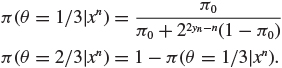
3. The predictive distribution of x_n+1 given xⁿ is

   

Before making any observation, the expected utility of immediately making a decision is

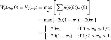
Therefore, the Bayes decision is a₀ if 1/2 ≤ π₀ ≤ 1 and a₁ if 0 ≤ π₀ ≤ 1/2. Figure 15.2 shows the V-shaped utility function V₀ highlighting that we expect to be better off at the extremes than at the center of the range of π₀ in addressing to choice of hypothesis.

Next, we calculate V₀(π_x¹), the value of taking an observation and then stopping. Suppose that x₁ has been observed. If x₁ = 0, the posterior expected utility is

Figure 15.2 Expected utility functions V₀ (solid), V₁ (dashed), and V₂ (dot–dashed) as functions of the prior probability π₀. Adapted from DeGroot (1970).

If x₁ = 1 the posterior expected utility is

Thus, the expected posterior utility is

Using the recursive relationship we derived in Section 15.3.3, we can derive the utility of the optimal procedure in which no more than one observation is taken. This is

If the prior is in the range 23/60 ≤ π₀ ≤ 37/60, the observation of x₁ will potentially move the posterior sufficiently to change the optimal decision, and to do so with sufficient confidence to offset the cost of observation.

The calculation of V₂ follows the same steps and works out so that

which leads to

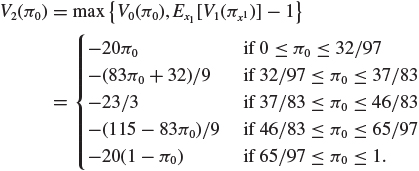
Because of the availability of the second observation, the range of priors for which it is optimal to start sampling is now broader, as shown in Figure 15.2.

To see how the solution works out in a specific case, suppose that π₀ = 0.48. With this prior, a decision with no data is a close call, so we expect the data to be useful. In fact, V₀(π₀) = − 9.60 < V₂(π₀) = − 7.67, so we should observe x₁. If x₁ = 0, we have V₀(π_x¹) = V₁(π_x¹) = − 7.03. Therefore, it is optimal to stop and choose a₀. If x₁ = 1, V₀(π_x¹) = V₁(π_x¹) = − 6.32 and, again, it is optimal to stop, but we choose a₁.

15.4.2 An example with equivalence between sequential and fixed sample size designs

This is another example from DeGroot (1970), and it shows that in some cases there is no gain from having the ability to accrue observations sequentially.

Suppose that x₁, x₂, ... is a sequential sample from a normal distribution with unknown mean θ and specified variance 1/ω. The parameter ω is called precision and is a more convenient way to handle this problem as we will see. Assume that θ is estimated under utility u(a(θ)) = −(θ – a)² and that there is a fixed cost c per observation. Also, suppose that the prior distribution π of θ is a normal distribution with mean μ and precision h. Then the posterior distribution of θ given xⁿ is normal with posterior precision h + nω. Therefore, there is no uncertainty about future utilities, as

and so V₀(π_xⁿ) = −1/(h+nω)for n = 0, 1, 2, .... This result shows that the expected utility depends only on the number of observations taken and not on their observed values. This implies that the optimal sequential decision procedure is a procedure in which a fixed number of observations is taken, because since the beginning we can predict exactly what our state of information will be at any stage in the process. Try Problem 15.3 for a more general version of this result.

Exploring this example a bit more, we discover that in this simple case we can solve the infinite horizon version of the dynamic programming solution to the optimal stopping rule. From our familiar recursion equation

Now

whenever

Using this fact, and an inductive argument (Problem 15.4), one can show that W_j(π, n) = − 1/(h + nω) – nc for β_n <ω ≤ β_n+1 where β_n is defined as β₀ = 0, β_n = c(h + (n – 1)ω)(h + nω) for n = 1, ..., j, and β_j+1 = ∞. This implies that the optimal sequential decision is to take exactly n^* observations, where n^* is an integer such that . If the decision maker is not allowed to take more than k observations, then if n^* > k, he or she should take k observations.

15.5 Sequential sampling to reduce uncertainty

In this section we discuss sampling rules that do not involve statements of costs of experimentation, following Lindley (1956) and DeGroot (1962). The decision maker’s goal is to obtain enough information about the parameters of interest. Experimentation stops when enough information is reached. Specifically, let V_x(E) denote the observed information provided by observing x in experiment E as defined in Chapter 13. Sampling would continue until V_xⁿ (E) ≥ 1/∊, with ∊ chosen before experimentation starts. In estimation under squared error loss, for example, this would mean sampling until Var[θ|xⁿ] < ∊ for some ∊.

Example 15.1 Suppose that Θ = {θ₀, θ₁} and let π = π(θ₀) and π_xn = π_xⁿ (θ₀). Consider the following sequential procedure: sampling continues until the Shannon information of π_xⁿ is at least ∊. In symbols, sampling continues until

For more details on Shannon information and entropy see Cover and Thomas (1991). One can show that Shannon’s information is convex in π_xⁿ. Thus, inequality (15.7) is equivalent to sampling as long as

with A′ and B′ satisfying the equality in (15.7). If π_xⁿ < A′, then we stop and accept H₁;if π_xⁿ > B′ we stop and accept H₀.

Rewriting the posterior in terms of the prior and likelihood,

This implies that inequality (15.8) is equivalent to

with

The procedure just derived is of the same form as Wald’s sequential probability ratio test (Wald 1947b), though in Wald the boundaries for stopping are determined using frequentist operating characteristics of the algorithm.

Example 15.2 Let x₁, x₂, ... be sequential observations from a Bernoulli distribution with unknown probability of success θ. We are interested in estimating θ under the quadratic loss function. Suppose that θ is a priori Beta(α₀, β₀), and let α_n and β_n denote the parameters of the beta posterior distribution. The optimal estimate of θ is the posterior mean, that is δ* = α_n/(α_n + β_n). The associated Bayes risk is the posterior variance Var[θ|xⁿ] = α_nβ_n/[(α_n + β_n)²(α_n + β_n + 1)].

Figure 15.3 shows the contour plot of the Bayes risk as a function of α_n and β_n. Say the sampling rule is to take observations as long as Var[θ|xⁿ] ≥ ∊ = 0.02. Starting with a uniform prior (α = β = 1), the prior variance is approximately equal to 0.08. The segments in Figure 15.3 show the trajectory of the Bayes risk after observing a particular sample. The first observation is a success and thus α_n = 2, β_n = 1, so our trajectory moves one step to the right. After n = 9 observations

Figure 15.3 Contour plot of the Bayes risk as a function of the beta posterior parameters α_n (labeled a) and β_n (labeled b).

with x = (1, 0, 0, 1, 1, 1, 0, 1, 1) the decision maker crosses the 0.02 curve, and stops experimentation.

For a more detailed discussion of this example, including the analysis of the problem using asymptotic approximations, see Lindley (1956) and Lindley (1957).

Example 15.3 Suppose that x₁, x₂, ... are sequentially drawn from a normal distribution with unknown mean θ and known variance σ ². Suppose that a priori θ has N(0, 1) distribution. The posterior variance Var[θ|xⁿ] = σ ²/(n + σ ²) is independent of xⁿ. Let 0 < ∊ < 1. Sampling until Var[θ|xⁿ] < is equivalent to taking a fixed sample size with n > σ ²(1 – ∊)/∊.

15.6 The stopping rule principle

15.6.1 Stopping rules and the Likelihood Principle

In this section we return to our discussion of foundation and elaborate on Theorem 15.1, which states that the Bayesian optimal decision is not affected by the stopping rule. The reason for this result is a general factorization of the likelihood: for any stopping rule ζ for sampling from a sequence of observations x₁, x₂, ... having fixed sample size parametric model f(xⁿ|n, θ) = f(xⁿ|θ), the likelihood function is

for all (n, xⁿ) such that f(n, xⁿ|θ) = 0.

Thus the likelihood function is the same irrespective of the stopping rule. The stopping time provides no additional information about θ to that already contained in the likelihood function f(xⁿ|θ) or in the prior π(θ), a fact referred to as the stopping rule principle (Raiffa and Schlaifer 1961). If one uses any statistical procedure satisfying the Likelihood Principle the stopping rule should have no effect on the final reported evidence about θ (Berger and Wolpert 1988):

Some of the difficulties faced by frequentist analysis will be illustrated with the next example (Berger and Wolpert 1988, pp. 74.1–74.2.). A scientist comes to the statistician’s office with 100 observations that are assumed to be independent and identically distributed N(θ, 1). The scientist wants to test the hypothesis H₀ : θ = 0 versus H₁ : θ = 0. The sample mean is , so that the test statistic is . At the level 0.05, a classical statistician could conclude that there is significant evidence against the null hypothesis.

With a more careful consultancy skill, suppose that the classical statistician asks the scientist the reason for stopping experimentation after 100 observations. If the scientist says that she decided to take only a batch of 100 observations, then the statistician could claim significance at the level 0.05. Is that right? From a classical perspective, another important question would be the scientist’s attitude towards a non-significant result. Suppose that the scientist says that she would take another batch of 100 observations thus, considering a rule of the form:

1. Take 100 observations.

2. If then stop and reject the null hypothesis.

3. If then take another 100 observations and reject the null hypothesis if .

This procedure would have level α = 0.05, with k = 2.18. Since , the scientist could not reject the null hypothesis and would have to take additional 100 observations.

This example shows that when using the frequentist approach, the interpretation of the results of an experiment depends not only on the data obtained and the way they were obtained, but also on the experimenter’s intentions. Berger and Wolpert comment on the problems faced by frequentist sequential methods:

15.6.2 Sampling to a foregone conclusion

One of the reasons for the reluctance of frequentist statisticians to accept the stopping rule principle is the concern that when the stopping rule is ignored, investigators using frequentist measures of evidence could be allowed to reach any conclusion they like by sampling until their favorite hypothesis receives enough evidence. To see how that happens, suppose that x₁, x₂, ... are sequentially drawn, normally distributed random variables with mean θ and unit variance. An investigator is interested in disproving the null hypothesis that θ = 0. She collects the data sequentially, by performing a fixed sample size test, and stopping when the departure from the null hypothesis is significant at some prespecified level α. In symbols, this means continue sampling until , where denotes the sample mean and k_α is chosen so that the level of the test is α. This stopping rule can be proved to be proper. Thus, almost surely she will reject the null hypothesis. This may take a long time, but it is guaranteed to happen. We refer to this as “sampling to a foregone conclusion.”

Kadane et al. (1996) examine the question of whether the expected utility theory, which leads to not using the stopping rule in reaching a terminal decision, is also prone to sampling to a foregone conclusion. They frame the question as follows: can we find, within the expected utility paradigm, a stopping rule such that, given the experimental data, the posterior probability of the hypothesis of interest is necessarily greater than its prior probability?

One thing they discover is that sampling to foregone conclusions is indeed possible when using improper priors that are finitely, but not countably, additive (Billingsley 1995). This means trouble for all the decision rules that, like minimax, are Bayes only when one takes limits of priors:

By contrast, though, if all distributions involved are countably additive, then, as you may remember from Chapter 10, the posterior distribution is a martingale, so a priori we expect it to be stable. Consider any real-valued function h. Assuming that the expectations involved exist, it follows from the law of total probability that

E_θ[h(θ)] = E_x[E_θ[h(θ)|x]].

So there can be no experiment designed to drive up or drive down for sure the conditional expectation of h, given x. Let h = I_{{θ∈ Θ0}} denote the indicator that θ belongs to Θ₀, the subspace defined by some hypothesis H₀, and let E_θ[h(θ)] = π(H₀) = π₀. Suppose that x₁, x₂, ... are sequentially observed. Consider a design with a minimum sample of size k ≥ 0 and define the stopping time N = inf{n ≥ k : π(H₀|xⁿ) ≥ q}, with N = ∞ if the set is empty. This means that sampling stops when the posterior probability is at least q. Assume that q > π₀. Then

where F(xⁿ|n) is the cumulative distribution of xⁿ given N = n. From the inequality above, P(N < ∞) ≤ π₀/q < 1. Then, with probability less than 1, a Bayesian stops the sequence of experiments and concludes that the posterior probability of hypothesis H₀ is at least q. Based on this result, a foregone conclusion cannot be reached for sure.

Now that we have reached the conclusion that our Bayesian journey could not be rigged to reach a foregone conclusion, we may stop.

15.7 Exercises

Problem 15.1 (Berger 1985) This is an application of optimal stopping in an estimation problem. Assume that x₁, x₂, ... is a sequential sample from a Bernoulli distribution with parameter θ. We want to estimate θ when the utility is u(θ, a, n) = −(θ – a)² – nc. Assume a priori that θ has a uniform distribution on (0,1). The cost of sampling is c = 0.01. Find the Bayes three-truncated procedure d³.

Solution

First, we will state without proof some basic results:

1. The posterior distribution of θ given xⁿ is a (, ).

2. Let . The marginal distribution of xⁿ is given by

   

3. The predictive distribution of x_n+1 given xⁿ is

   

Now, since the terminal utility is u(a(θ)) = −(θ – a)², the optimal action a* is the posterior mean, and the posterior expected utility is minus the posterior variance. Therefore,

Using this result,

Observe that

Note that

and, similarly,

Thus,

Proceeding similarly, we find,

We can now describe the optimal three-truncated Bayes procedure. Since at stage 0, W₀(π,0) = −0.083 < W₃(π,0) = −0.0617, x₁ should be observed. After observing x₁, as W₀(π_x¹,1) = − 0.0655 < W₂(π_x¹,1) = − 0.0617, we should observe x₂. After observing it, since we have W₀(π_x²,2) = W₁(π_x², 2), it is optimal to stop. The Bayes action is

Problem 15.2 Sequential problems get very hard very quickly. This is one of the simplest you can try, but it will take some time. Try to address the same question as the worked example in Problem 15.1, except with Poisson observations and a Gamma(1, 1) prior. Set c = 1/12.

Problem 15.3 (From DeGroot 1970) Let π be the prior distribution of θ in a sequential decision problem. (a) Prove by using an inductive argument that, in a sequential decision problem with fixed cost per observation, if V₀(π_xⁿ) is constant for all observed values xⁿ, then every function V_j for j = 1, 2, ... as well as V₀ has this property. (b) Conclude that the optimal sequential decision procedure is a procedure in which a fixed number of observations are taken.

Problem 15.4 (From DeGroot 1970) (a) In the context of Example 15.4.2, for n = 0, 1, ..., j, prove that

where β_n is defined as β₀ = 0, β_n = c(h + (n – 1)ω)(h + nω) for n = 1, ..., j and β_j+1 = ∞. (b) Conclude that if the decision maker is allowed to take no more than k observations, then the optimal procedure is to take n* ≤ k observations where n* is such that β_n* < ω ≤ β_n*+1.