

If s is even, then 2k+1 | n−1and![]() mod n. Otherwise, if s is odd, then 2k+1 ∤ n−1 and
mod n. Otherwise, if s is odd, then 2k+1 ∤ n−1 and ![]() mod n. Euler’s criterion and Zolotarev’s lemma yield
mod n. Euler’s criterion and Zolotarev’s lemma yield
Thus, ![]() We conclude
We conclude ![]() mod n, as desired.
mod n, as desired.
□
The proof of Theorem 3.12 is adapted from Carl Bernard Pomerance (born 1944), John Lewis Selfridge (1927–2010), and Samuel Standfield Wagstaff, Jr. (born 1945) [85].
3.5 Extracting roots in finite fields
Extracting roots in a group G is the following problem. Let an element a ∈ G be given, which is known to be a square, that is, an element b ∈ G with a = b2 exists. The goal is to determine such an element b satisfying a = b2. In general, the solution is not unique. It is often difficult to extract roots modulo n. In this section, we show that in finite fields, this problem is efficiently solvable using probabilistic algorithms. Let ![]() be a finite field. On input a ∈
be a finite field. On input a ∈ ![]() ,wewant to compute b ∈
,wewant to compute b ∈ ![]() with b2 = a. We call b a square root of a and say that a is a square or a quadratic residue. If b is a root of a, then so is −b. Since quadratic equations over fields have at most two solutions, we conclude that b and −b are the only roots of a. There are some special cases where extracting roots is particularly simple. Before we examine a general method, let us first consider two such special cases.
with b2 = a. We call b a square root of a and say that a is a square or a quadratic residue. If b is a root of a, then so is −b. Since quadratic equations over fields have at most two solutions, we conclude that b and −b are the only roots of a. There are some special cases where extracting roots is particularly simple. Before we examine a general method, let us first consider two such special cases.
Let G be a finite group of odd order and a ∈ G. We let b = a(|G|+1)/2. The crucial point here is that (|G| + 1)/2 is an integer. From Corollary 1.5, we have a|G| = 1. Thus, b2 = a|G|a = a. So b is a square root of a. This covers the case![]() =
= ![]() 2n because here the order of the multiplicative group
2n because here the order of the multiplicative group ![]() ∗ =
∗ = ![]() {0} is odd. In particular, each element in 2n is a square.
{0} is odd. In particular, each element in 2n is a square.
Before we proceed to the second special case, we want to remark that, in general, not every element of a field is a square. A simple example for that is ![]() 3 = {0, 1, −1}. In this field, −1 is not a square. We can use Euler’s criterion to check whether an element a of a field ' with an odd number of elements is a square: we have a(|
3 = {0, 1, −1}. In this field, −1 is not a square. We can use Euler’s criterion to check whether an element a of a field ' with an odd number of elements is a square: we have a(|![]() |−1)/2 = 1 if and only if a is a square. We now investigate the case || ≡ −1 mod 4 separately since, in this case, extracting roots is simple. The reason is that exactly one of the elements a and −a in
|−1)/2 = 1 if and only if a is a square. We now investigate the case || ≡ −1 mod 4 separately since, in this case, extracting roots is simple. The reason is that exactly one of the elements a and −a in ![]() ∗ is a square: since |
∗ is a square: since |![]() | + 1 is divisible by 4, the element b = a(|
| + 1 is divisible by 4, the element b = a(|![]() |+1)/4 is well defined and we have
|+1)/4 is well defined and we have

Thus, if a is a square, then b is one of its square roots. Next, we consider two algorithms to extract roots in arbitrary finite fields ' for which || is odd.
3.5.1 Tonelli’s algorithm
Let ![]() be a finite field with an odd number q = || of elements. We present the probabilistic method for extracting roots, as developed by Alberto Tonelli (1849–1921) in 1891. To this end, we write q − 1 = 2ℓu with u odd. Let
be a finite field with an odd number q = || of elements. We present the probabilistic method for extracting roots, as developed by Alberto Tonelli (1849–1921) in 1891. To this end, we write q − 1 = 2ℓu with u odd. Let
Each set Gi−1 is a subgroup of Gi, and Gℓ = ![]() ∗. Since ∗ is cyclic, all groups Gi are cyclic, too. Let x be a generator of
∗. Since ∗ is cyclic, all groups Gi are cyclic, too. Let x be a generator of ![]() ∗. Then, x2ℓ−i is a generator of Gi. In particular, we can see that the index of Gi−1 in Gi is 2.
∗. Then, x2ℓ−i is a generator of Gi. In particular, we can see that the index of Gi−1 in Gi is 2.
Let g ∈ ![]() ∗ be not a square. With Euler’s criterion, we obtain
∗ be not a square. With Euler’s criterion, we obtain ![]()
![]() Thus,
Thus, ![]() and, moreover, Gℓ−i−1 and g2i Gℓ−i−1 are the two cosets of Gℓ−i−1 in Gℓ−i; that is, you can alternate between these two cosets by multiplication with g2i. Each quotient Gi/Gi−1 is generated by a power of g. Thus, also
and, moreover, Gℓ−i−1 and g2i Gℓ−i−1 are the two cosets of Gℓ−i−1 in Gℓ−i; that is, you can alternate between these two cosets by multiplication with g2i. Each quotient Gi/Gi−1 is generated by a power of g. Thus, also ![]() ∗/ G0 is generated by g. In particular, each element a ∈
∗/ G0 is generated by g. In particular, each element a ∈ ![]() ∗ can be written as a = gkh with h ∈ G0. The idea now is to extract the roots of gk and h separately. For h, this is easy because G0 is of odd order. If a is a square, then k is even: Euler’s criterion yields
∗ can be written as a = gkh with h ∈ G0. The idea now is to extract the roots of gk and h separately. For h, this is easy because G0 is of odd order. If a is a square, then k is even: Euler’s criterion yields
and, because of ![]() we see that k must be even, showing that gk/2 is a root of gk. Therefore, it only remains to determine the exponent k. Let k = Σj≥0 kj2j be the binary representation of k. For the first i bits k0, . . . , ki−1 of k, using
we see that k must be even, showing that gk/2 is a root of gk. Therefore, it only remains to determine the exponent k. Let k = Σj≥0 kj2j be the binary representation of k. For the first i bits k0, . . . , ki−1 of k, using ![]() we obtain
we obtain
This shows that ![]() If k0, . . . , ki−2 are known already, then the bit ki−1 is uniquely determined, because
If k0, . . . , ki−2 are known already, then the bit ki−1 is uniquely determined, because ![]() Finally, this yields the following algorithm:
Finally, this yields the following algorithm:
(1)Choose a random element g ∈ ∗ until g is not a square.
(2)Determine k0, . . . , kℓ−1 successively such that ![]() for all i.
for all i.
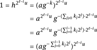
(3)Let ![]() and h = ag−k.
and h = ag−k.
(4)Return b = gk/2 h(u+1)/2 as a root of a.
In each iteration of the first step, g is not a square with probability 1/2. Therefore, a suitable g is found after only a few rounds with high probability. To check whether c ∈ Gℓ−i, we compute c2ℓ−iu. Using fast exponentiation, this takes O(log q) operations in . The test has to be carried out ℓ times, so ![]() (ℓ log q) operations in ' suffice for this part. Since ℓ ≤ log q, the worst case here is O(log2 q) operations. The remaining steps are in O(log q).
(ℓ log q) operations in ' suffice for this part. Since ℓ ≤ log q, the worst case here is O(log2 q) operations. The remaining steps are in O(log q).
This can be slightly improved using a trick of Daniel Shanks (1917–1996). For this purpose, we compute c = au. The element gu is not a square since
Replacing g by gu, after step (1) of Tonelli’s algorithm, we may assume that ![]() The condition
The condition ![]() now is equivalent to
now is equivalent to ![]() This can be checked using
This can be checked using ![]() (ℓ) field operations. Thus, the complexity of the algorithm is improved to
(ℓ) field operations. Thus, the complexity of the algorithm is improved to ![]() (ℓ2 + log q) operations in .
(ℓ2 + log q) operations in .
3.5.2 Cipolla’s algorithm
Let ![]() be a finite field with an odd number of elements. We now present and investigate the randomized algorithm of Michele Cipolla (1880–1947) for finding a square root. This algorithm works with polynomials in [X]. On input a ∈ , the idea is to construct a field extension in which it is easy to compute a square root of a. In the following, let the input a ∈
be a finite field with an odd number of elements. We now present and investigate the randomized algorithm of Michele Cipolla (1880–1947) for finding a square root. This algorithm works with polynomials in [X]. On input a ∈ , the idea is to construct a field extension in which it is easy to compute a square root of a. In the following, let the input a ∈ ![]() ∗ be a square:
∗ be a square:
(1)Repeatedly choose elements t ∈ ' at random until t2 − 4a is not a square.
(2)Let f = X2 − tX + a.
(3)Compute b = X(||+1)/2 mod f . This is the desired square root of a.
We first show that, with high probability, a suitable element t is chosen in the first step.
Theorem 3.13. Let a ∈ ![]() ∗ be a square. If t ∈ ' is randomly chosen, then t2 − 4a is not a square with probability (|
∗ be a square. If t ∈ ' is randomly chosen, then t2 − 4a is not a square with probability (|![]() | − 1)/(2|
| − 1)/(2|![]() |).
|).
Proof: By completing the square, we see that t2 − 4a is a square if and only if the polynomial X2 − tX + a splits into linear factors over . The number of polynomials X2 − tX + a with t ∈ ' that split into linear factors over ' is equal to the number of polynomials (X−α)(X−β) with αβ = a. If you choose α, then β is uniquely determined (since a ≠ 0). We have α = β if and only if α is one of the two square roots of a. There are |![]() |−3 different ways to choose α such that α ≠ β and αβ = a. Due to the symmetry in α and β, this yields (|
|−3 different ways to choose α such that α ≠ β and αβ = a. Due to the symmetry in α and β, this yields (|![]() | − 3)/2 polynomials. Additionally, there are the two possibilities for α = β being a square root of a. The remaining (|
| − 3)/2 polynomials. Additionally, there are the two possibilities for α = β being a square root of a. The remaining (|![]() | − 1)/2 polynomials do not split into linear factors. This proves the statement of the theorem.
| − 1)/2 polynomials do not split into linear factors. This proves the statement of the theorem.
□
If t2 − 4a is not a square, then the polynomial f = X2 − tX + a ∈ ![]() [X] is irreducible. Using Theorem 1.51, we see that
[X] is irreducible. Using Theorem 1.51, we see that ![]() =
= ![]() [X]/f is a field that contains . The field ' contains X as an element. An important property of the element X ∈ is provided by the following theorem.
[X]/f is a field that contains . The field ' contains X as an element. An important property of the element X ∈ is provided by the following theorem.
Theorem 3.14. In , we have X|![]() |+1 = a.
|+1 = a.
Proof: If |![]() | = pq for some prime p, then the mapping φ:
| = pq for some prime p, then the mapping φ: ![]() →
→ ![]() with φ(x) = x|
with φ(x) = x|![]() | is the q-fold application of the Frobenius homomorphism x ↦ xp; see Theorem 1.28. In particular, φ is a homomorphism. Since the roots of the polynomial Y|
| is the q-fold application of the Frobenius homomorphism x ↦ xp; see Theorem 1.28. In particular, φ is a homomorphism. Since the roots of the polynomial Y|![]() | − Y ∈
| − Y ∈ ![]() [Y] are exactly the elements of
[Y] are exactly the elements of ![]() , we see that φ(x) = x if and only if x ∈
, we see that φ(x) = x if and only if x ∈ ![]() .
.
Consider the polynomial h = Y2 − tY + a ∈ ![]() [Y]. The roots of this polynomial are X and t−X. Since the coefficients of h are in, the elements φ(X) and φ(t−X) are roots of h, too. For instance, we have 0 = φ(0) = φ(h(X)) = φ(X)2 − tφ(X) + a. We conclude {X, t − X} = {φ(X), φ(t − X)}. Now, X ∉
[Y]. The roots of this polynomial are X and t−X. Since the coefficients of h are in, the elements φ(X) and φ(t−X) are roots of h, too. For instance, we have 0 = φ(0) = φ(h(X)) = φ(X)2 − tφ(X) + a. We conclude {X, t − X} = {φ(X), φ(t − X)}. Now, X ∉ ![]() yields φ(X) ≠ X and thus X|
yields φ(X) ≠ X and thus X|![]() | = φ(X) = t − X. Finally, we obtain X|
| = φ(X) = t − X. Finally, we obtain X|![]() |+1 = XX|
|+1 = XX|![]() | = X(t − X) = a.
| = X(t − X) = a.
From Theorem3.13, it follows that, with high probability after a few runs, the algorithm will find a suitable element t ∈ ![]() . Therefore, Cipolla’s algorithm can be performed efficiently. Once t is found, the algorithm executes O(log |
. Therefore, Cipolla’s algorithm can be performed efficiently. Once t is found, the algorithm executes O(log |![]() |) field operations. From Theorem 3.14, we see that b ∈ is a square root of a. Now a, by assumption, has two square roots in . But since the equation Y2 = a has only two solutions, it follows that b ∈
|) field operations. From Theorem 3.14, we see that b ∈ is a square root of a. Now a, by assumption, has two square roots in . But since the equation Y2 = a has only two solutions, it follows that b ∈ ![]() . This shows the validity of Cipolla’s algorithm.
. This shows the validity of Cipolla’s algorithm.
□
If a ∈ ![]() ∗ is not a square, then Cipolla’s algorithm still computes a square root b of a, but in this case we have b ∈
∗ is not a square, then Cipolla’s algorithm still computes a square root b of a, but in this case we have b ∈ ![]() . Also, note that if a is not a square, then the success probability for finding an appropriate t is (|
. Also, note that if a is not a square, then the success probability for finding an appropriate t is (|![]() |+1)/(2|
|+1)/(2|![]() |); this is slightly better than in the case of a being a square.
|); this is slightly better than in the case of a being a square.
3.6 Integer factorization
The security of many cryptosystems is based on the assumption that it is impossible to factorize large numbers efficiently. In this chapter, we will introduce some methods to demonstrate that the factorization of certain numbers is easy; from that we immediately obtain criteria for poorly chosen keys in certain cryptosystems. To factorize a number n one needs to find a factor m of n with 1 < m < n. To completely decompose n into its prime factors, one can go on by factorizing m and n /m. Before starting to factorize a number n, one can use a primality test like the Miller–Rabin test to check whether n is composite at all.
3.6.1 Pollard’s p − 1 algorithm
An idea of John Michael Pollard for factorization is the following. Let p be a prime divisor of n. With Fermat’s little theorem, we obtain ak ≡ 1 mod p for all multiples k of p −1. If p −1 contains only prime factors of a set B, then we can use ![]() Frequently, B is chosen to be the set of all primes up to a certain size. If ak ≢ 1 mod n, we obtain a nontrivial divisor of n by computing gcd(ak − 1, n). This leads to the following algorithm to find a divisor of n:
Frequently, B is chosen to be the set of all primes up to a certain size. If ak ≢ 1 mod n, we obtain a nontrivial divisor of n by computing gcd(ak − 1, n). This leads to the following algorithm to find a divisor of n:
(1)Let ![]()
(2)Compute gcd(ak − 1, n) for a randomly chosen a ∈ {2, . . . , n − 1}.
(3)If this does not yield a proper divisor of n, then try a new value of a or a larger base B of prime numbers.
Of course, in step(2),we first compute b = ak mod n with fast modular exponentiation and then gcd(b−1, n). The problem with Pollard’s p −1 algorithm is that the structure of the group (ℤ/nℤ)∗ is fixed. If no prime divisor p of n has the property that p −1 has only small prime factors, then this method does not work. Using an overlarge base B makes k huge, and thus the algorithm becomes inefficient.
3.6.2 Pollard’s rho algorithm for factorization
Another idea of Pollard’s for integer factorization uses the birthday paradox. The basic idea behind so-called ρ algorithms is as follows. From the birthday paradox, there is a high probability that in a sequence of ![]() random elements from a finite set M two chosen elements are the same. Instead of a random sequence, you determine a pseudo-random sequence m0, m1, . . . with the property that mi+1 can be uniquely determined from mi. Then, if mi = mj, we obtain mi+k = m j+k for all k ≥ 0. Moreover, from the viewpoint of an observer m0, m1, . . . , should behave like a random sequence. In particular, the probability of finding two indices i < j with mi = m j after
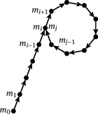
random elements from a finite set M two chosen elements are the same. Instead of a random sequence, you determine a pseudo-random sequence m0, m1, . . . with the property that mi+1 can be uniquely determined from mi. Then, if mi = mj, we obtain mi+k = m j+k for all k ≥ 0. Moreover, from the viewpoint of an observer m0, m1, . . . , should behave like a random sequence. In particular, the probability of finding two indices i < j with mi = m j after ![]() steps is high. The shape of the image below motivates the term “ρ algorithm.”
steps is high. The shape of the image below motivates the term “ρ algorithm.”
Assume that n has a prime divisor p, and let f : ℤ/pℤ → ℤ/pℤ be an arbitrary mapping. The target set of f being finite, there exist integers j > i ≥ 0 with f j(x0) = f i(x0). If f behaves sufficiently randomly, then, with high probability, this phenomenon will already occur after the first ![]() steps. The function f(x) = x2 + a mod p with a ∉ {−2, −1, 0} is often used; f(x) = x2 + 1 mod p is a typical example. As, unfortunately, we do not know p yet, we compute F (x) = x2 + a mod n instead of f. This yields
steps. The function f(x) = x2 + a mod p with a ∉ {−2, −1, 0} is often used; f(x) = x2 + 1 mod p is a typical example. As, unfortunately, we do not know p yet, we compute F (x) = x2 + a mod n instead of f. This yields
Now, we hope to find two elements that are the same in the f -sequence, but different in the F-sequence. For the corresponding indices i ≠ j, we have
Using this pair (i, j), we now obtain a nontrivial factor of n by computing gcd(Fj(x0)−F i(x0), n). The problem is that storing each of the F i(x0) is too expensive, as is the comparison of all F i(x0) with each other. The solution is to continually increase the distance which we suspect is between i and j. Let xi = Fi(x0) and yi = F2i(x0). If xi ≡ xi+k mod p, then we obtainxj ≡ xj+k mod p for all j ≥ i. In particular, for j = kℓ ≥ i we have xj ≡ x2j = yj mod p. This leads to the following algorithm:
(1)Choose x0 ∈ {0, . . . , n − 1} at random, and let y0 = x0.
(2)For all i ≥ 1, successively consider the pairs
and check whether gcd(yi − xi , n) yields a nontrivial divisor of n.
(3)Once gcd(yi − xi , n) = n holds, the procedure is stopped and restarted with a new initial value x0 or a different function F.
If gcd(yi−xi , n) = n holds, then we have found a cycle for the F-sequence. The problem is that the ρ algorithm for factorization is only efficient if n has a sufficiently small prime factor p. The expected number of arithmetic operations of the procedure to find a divisor of n is ![]() If the smallest prime divisor is of order
If the smallest prime divisor is of order ![]() then
then ![]() operations have to be carried out. This is not feasible for large integers.
operations have to be carried out. This is not feasible for large integers.
3.6.3 Quadratic sieve
The quadratic sieve is a factorization algorithm which does not require the input n to have some special structure. The basic idea is to find integers x and y such that x2 ≡ y2 mod n and x ≢ ±y mod n. In this case, both gcd(x − y, n) and gcd(x + y, n) yield a nontrivial factor of n.
We first fix a factor base B consisting of −1 together with a list of prime numbers. A typical choice is
for some bound b depending on n. An integer is B-smooth if it can be written as a product of elements in B. In the first phase, we compute a large set of numbers S such that r2 mod n is B-smooth for all r ∈ S. Then, in the second phase, we choose a subset T of S such that all prime exponents in Πr∈T(t2 mod n) are even. Finally, we set x = Πr∈T r and y is computed from Πr∈T(r2 mod n) by halving all prime exponents. By construction, we have x2 ≡ y2 mod n. However, if x ≡ ±y mod n, then we either have to try a different choice for T, compute an even larger set S, or start all over again with a bigger bound b.
Let us consider the first phase in more detail. Let ![]() and
and
for some bound c significantly smaller than m /2. We define f(r) = r2 −n for r ∈ R. Note that |f(r)| is in the order of magnitude of 2cm < n. We want to compute
For every element r ∈ S, there is a factorization
The computation of S starts with the vector (f(−c + m), . . . , f(c + m)). For every prime p ∈ B, if some entry in this vector is divisible by p, we divide it by p as often as possible. If we end up with an entry 1 or −1, then the initial integer at this position is B-smooth. Note that this computation also gives the prime exponents ep,s. It is too costly to check for every entry whether it is divisible by p. Here, the sieving comes into play. The entry f(r) is divisible by p if and only if f(r) = r2 − n ≡ 0 mod p. We compute solutions r1 and r2 of the quadratic equation r2 ≡ n mod p; this can be achieved with Tonelli’s or Cipolla’s algorithm from Section 3.5. We have ![]() mod p, and f(r) is divisible by p if and only if r ∈ {r1, r2} + pℕ. By construction of the vector, it suffices to consider c/p entries.
mod p, and f(r) is divisible by p if and only if r ∈ {r1, r2} + pℕ. By construction of the vector, it suffices to consider c/p entries.
In the second phase, we want to compute a subset T ⊆ S such that in the product
all exponents Σr∈T ep,r for p ∈ B are even (including the exponent of −1). To this end, we need to find a nontrivial solution of the following system of linear equations modulo 2 with variables Xr ∈ {1, 0}:
In particular, we want to have |S| ≥ |B|. The set T is given by
Finally, we set x = Πr∈T r and y = Πp∈B p(Σr∈T ep,r)/2.
If B is too small, we have to choose a huge c in order to have |S| ≥ |B|. On the other hand, if B is large, the sieving takes a lot of time and we have to solve a large system of linear equations. Typically, you start with rather “small” values of b and c in the order of magnitude of ![]() and then increases them if the algorithm does not succeed with the factorization of n.
and then increases them if the algorithm does not succeed with the factorization of n.
There are many optimizations of the quadratic sieve. For instance, it suffices to only consider primes p in the factor base such that n modulo p is a square; otherwise the quadratic equation r2 ≡ n mod p has no solution.
Example 3.15. Let n = 91. We consider the factor base B = {−1, 2, 3, 5}. With m = 9 and c = 2, we obtain R = {7, 8, 9, 10, 11}. For r ∈ R , we compute f(r) = r2 − 91. This yields the initial vector (f(7), . . . , f(11)) = (−42, −27, −10, 9, 30). The following table summarizes the sieving stage.

The B-smooth numbers are −27 = (−1) ⋅ 33 and −10 = (−1) ⋅ 2 ⋅ 5 and 9 = 32 and 30 = 2 ⋅ 3 ⋅ 5. Possible choices for T are T1 = {8, 9, 10, 11} and T2 = {8, 9, 11} and T3 = {10}. For T1, we obtain x1 = 8⋅9⋅10⋅11 = 7920 and y1 = 2⋅33 ⋅5 = 270; we can omit the sign of y1 since both +y1 and −y1 are considered. We have gcd(x1−y1, 91) = 1 and gcd(x1 + y1, 91) = 91. Therefore, T1 does not yield a factorization of 91. For T2, we obtain x2 = 8 ⋅ 9 ⋅ 11 = 792 and y2 = 2 ⋅ 32 ⋅ 5 = 90. This yields the factorization 91 = 13 ⋅ 7 since gcd(x2 − y2, 91) = 13 and gcd(x2 + y2, 91) = 7. Finally, for T3, we obtain x3 = 10 and y3 = 3. This immediately yields the factors x3 − y3 = 7 and x3 + y3 = 13.
◊
3.7 Discrete logarithm
Currently, no efficient methods for integer factorization are known, and it is widely believed that no such methods exist. The security of many cryptosystems depends heavily on this assumption. However, you cannot completely rule out the possibility that one day factorizing can be done sufficiently fast. Therefore, we are interested in cryptosystems whose security is based on the hardness of other computational problems. One such problem is the discrete logarithm.
Let G be a group and g ∈ G an element of order q. Let U be the subgroup of G generated by g, so |U| = q. Then, x ↦ gx defines an isomorphism ℤ/qℤ → U which can be computed using fast exponentiation in many applications. The discrete logarithm problem is the task of determining the element x mod q from the knowledge of the elements g and gx in G. If G is the additive group (ℤ/nℤ, +, 0), this is easy using the extended Euclidean algorithm. But what should be done when the Euclidean algorithm is not available? It seems that, then, the inverse mapping of x ↦ gx cannot be computed efficiently. In applications, it is therefore sufficient to work with the multiplicative group of a finite field or a finite group of points on an elliptic curve. With elliptic curves, you can apparently reach the same level of security with fewer bits, but since we have not yet dealt with elliptic curves, wewill restrict ourselves to the case ∗p for a prime number p.
We fix the prime number p and the element ![]() Let the order of g in
Let the order of g in ![]() be q. Then, in particular, q is a divisor of p − 1. Suppose we are given
be q. Then, in particular, q is a divisor of p − 1. Suppose we are given ![]() The task is to determine x' ≤ p − 1 with
The task is to determine x' ≤ p − 1 with ![]() The naive method is to exhaustively try out all possible values for x. The expected search time is approximately q/2. This is hopeless if q,written in binary, has a length of 80 bits or more. In typical applications, q and p have a bit size of about 160 to 1000 bits each. The computation of xy mod z is very efficient when using fast modular exponentiation, even for numbers x, y, z with more than 1000 bits. Therefore, the mapping ℤ/qℤ → U with x ↦ gx can, in fact, be computed efficiently. The currently known algorithms for the discrete logarithm problem on inputs of bit size log n achieve a runtime of
The naive method is to exhaustively try out all possible values for x. The expected search time is approximately q/2. This is hopeless if q,written in binary, has a length of 80 bits or more. In typical applications, q and p have a bit size of about 160 to 1000 bits each. The computation of xy mod z is very efficient when using fast modular exponentiation, even for numbers x, y, z with more than 1000 bits. Therefore, the mapping ℤ/qℤ → U with x ↦ gx can, in fact, be computed efficiently. The currently known algorithms for the discrete logarithm problem on inputs of bit size log n achieve a runtime of ![]() on elliptic curves. This is considered to be subexponential and is significantly better than
on elliptic curves. This is considered to be subexponential and is significantly better than ![]() (n), but still too slow to treat 160-digit numbers reasonably. Note that a 160-digit number has an order of magnitude of 2160.
(n), but still too slow to treat 160-digit numbers reasonably. Note that a 160-digit number has an order of magnitude of 2160.
3.7.1 Shanks’ baby-step giant-step algorithm
Let G be a finite group of order n, let g ∈ G be an element of order q, and let y be a power of g. We search for a number x with gx = y, the discrete logarithm of y to base g. A classical algorithm to compute the discrete logarithm is the baby-step giant-step algorithm by Shanks. Here, a number m ∈ ℕ is chosen, which should be of approximate size ![]() If q is unknown, you can instead choose m to have approximate size
If q is unknown, you can instead choose m to have approximate size ![]() and substitute q by n in the following. For all r ∈ {m−1, . . . ,0} in the baby steps, one computes the values g−r = gq−r ∈ G and stores the pairs (r, yg−r ) in a table B. In practical implementations, you should use hash tables for efficiency reasons.
and substitute q by n in the following. For all r ∈ {m−1, . . . ,0} in the baby steps, one computes the values g−r = gq−r ∈ G and stores the pairs (r, yg−r ) in a table B. In practical implementations, you should use hash tables for efficiency reasons.
Note that for exactly one r with 0 ≤ r < m there is a number s with x = sm + r. Substituting z = yg−r, the pair (r, z) is in the table and z = gsm. The giant steps are as follows. We compute h = gm, and then for all s with 0 ≤ s < ⌈q/m⌉, we check whether a table entry (r, hs) exists. If we find such numbers r and s, then x = sm + r is the desired value.
The running time is dominated by m, that is, approximately ![]() or
or ![]() respectively. This is not particularly pleasing, but no faster methods are known. A bigger problem with this method is the huge amount of memory needed to store the m pairs (r, z). Even if you can reduce the table size by hashing and other elaborate methods, an enormous amount of data still have to be maintained and stored. For realistic sizes like q ≥ 2100, the baby-step giant-step algorithm is not feasible.
respectively. This is not particularly pleasing, but no faster methods are known. A bigger problem with this method is the huge amount of memory needed to store the m pairs (r, z). Even if you can reduce the table size by hashing and other elaborate methods, an enormous amount of data still have to be maintained and stored. For realistic sizes like q ≥ 2100, the baby-step giant-step algorithm is not feasible.
3.7.2 Pollard’s rho algorithm for the discrete logarithm
As before, let G be a finite group of order n, let g ∈ G be an element of order q, and y a power of g. We search for a number x with gx = y. The runtime of Pollard’s ρ algorithm to compute x is similar to that of Shanks’ baby-step giant-step algorithm; however, it requires only a constant amount of storage space. The price for this advantage is that the ρ algorithm yields no worst-case time bound, but rather a bound that is based on the birthday paradox. It only provides an expected time complexity of ![]()
First, we decompose G into three disjoint sets, P1, P2 and P3. In ![]() for example, you could define the Pi by residues modulo 3. In principle, the exact decomposition is irrelevant, but it should be easy to compute and ensure that the following scheme yields something like a random walk through the subgroup of G generated by g. We think of a pair (r, s) ∈ ℤ/qℤ×ℤ/qℤ as a representation of grys ∈ G. The above partition defines a mapping f : ℤ/qℤ×ℤ/qℤ→ℤ/qℤ×ℤ/qℤ as follows:
for example, you could define the Pi by residues modulo 3. In principle, the exact decomposition is irrelevant, but it should be easy to compute and ensure that the following scheme yields something like a random walk through the subgroup of G generated by g. We think of a pair (r, s) ∈ ℤ/qℤ×ℤ/qℤ as a representation of grys ∈ G. The above partition defines a mapping f : ℤ/qℤ×ℤ/qℤ→ℤ/qℤ×ℤ/qℤ as follows:
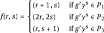
Let f(r, s) = (r' , s) and h = grys and ![]() then h' = gh for h ∈ P1, h' = h2 for h ∈ P2 and h' = hy for h ∈ P3. The ρ algorithm starts with a random pair (r1, s1) and iterates the computation by
then h' = gh for h ∈ P1, h' = h2 for h ∈ P2 and h' = hy for h ∈ P3. The ρ algorithm starts with a random pair (r1, s1) and iterates the computation by
for i ≥ 1. We define ![]() and observe that hi+1 can uniquely be determined from hi. Therefore, the sequence (h1, h2, . . . ) in G encounters a cycle after a finite initial segment and, therefore, it looks like the Greek letter ρ, again explaining the name of the algorithm.
and observe that hi+1 can uniquely be determined from hi. Therefore, the sequence (h1, h2, . . . ) in G encounters a cycle after a finite initial segment and, therefore, it looks like the Greek letter ρ, again explaining the name of the algorithm.
There exist t and r with ht = ht+r. Now hℓ = hℓ+r holds for all ℓ ≥ t. We use this fact to keep the required storage space bounded by a constant. We could proceed as we did in Section 3.6.2 to find different indices i, j with hi = hj. However, we want to use an alternative approach, which could also be used in the ρ algorithm for factorization. We work in phases: at the beginning of each phase, a value hℓ is stored. In the first phase, we let ℓ = 1. Then, for k ∈ {1, . . . , ℓ}, we successively compute the value hℓ+k and compare it with hℓ.We stop the procedure if ℓ is found such that hℓ = hℓ+k. Otherwise, we replace hℓ by h2ℓ and ℓ by 2ℓ and start a new phase. Note that, at the latest, we will stop if ℓ is greater than or equal to t + r because then, with k = r, we reach the situation hℓ = hℓ+k.
Thus, we stop with the pairs (r, s) = (rℓ , sℓ) and (r' , s) = (rℓ+k , sℓ+k), for which ![]() This implies
This implies ![]() and therefore r + xs ≡ r' + xs' mod q. Now, x(s−s) ≡ r−r mod q. The probability for s = s' is small and if q is prime, we can solve the congruence uniquely. This method, however, can also be applied to more general situations and we might possibly obtain different x to solve the last congruence. If possible, we check for all these solutions x whether gx = y holds. Otherwise, we restart the procedure, using another random pair (r1, s1).
and therefore r + xs ≡ r' + xs' mod q. Now, x(s−s) ≡ r−r mod q. The probability for s = s' is small and if q is prime, we can solve the congruence uniquely. This method, however, can also be applied to more general situations and we might possibly obtain different x to solve the last congruence. If possible, we check for all these solutions x whether gx = y holds. Otherwise, we restart the procedure, using another random pair (r1, s1).
The analysis of the running time depends on the expected minimal value t + r, yielding ht = ht+r. If the sequence (h1, h2, . . . ) behaves randomly, then we look for k such that the probability for the existence of ht = ht+r with 1 ≤ t < t + r ≤ k is greater than 1/2. The birthday paradox leads to an expected running time of ![]() for Pollard’s ρ algorithm.
for Pollard’s ρ algorithm.
3.7.3 Pohlig–Hellman algorithm for group order reduction
If the prime factorization of the order of a cyclic group G is known, then the discrete logarithm problem can be reduced to the prime divisors. The according method was published by Stephen Pohlig and Martin Hellman. Let |G| = n with
where the product runs over all prime divisors p of n. Let y, g ∈ G be given such that y is a power of g. We look for a number x with y = gx. We define
The elements Gp = {hnp | h ∈ G } form a subgroup of G. If h generates G, then hnp generates Gp. In particular, Gp contains exactly pe(p) elements. The following theorem shows that it is sufficient to solve the discrete logarithm problem in the groups Gp.
Theorem 3.16. For all primes p with p | n let xp ∈ ℕ be given such that ![]() If x ≡ xp mod pe(p) for all primes p | n, then y = gx.
If x ≡ xp mod pe(p) for all primes p | n, then y = gx.
Proof: We have ![]() Thus, the order of g−xy is a divisor of np for all p | n. The greatest common divisor of all np is 1, so the order of g−xy also must be 1. This shows y = gx.
Thus, the order of g−xy is a divisor of np for all p | n. The greatest common divisor of all np is 1, so the order of g−xy also must be 1. This shows y = gx.
□
With the Chinese remainder theorem from Theorem 3.16, we can compute a solution in G from the solutions in the groups Gp. We further simplify the problem for Gp by reducing the discrete logarithm to groups of order p. Without loss of generality let now |G| = pe for a prime number p. Since x < pe, there exists a unique representation
with 0 ≤ xi < p. We successively compute x0, . . . , xe−1 as follows. Let x0, . . . , xi−1 be known already for i ≥ 0. For ![]() we have
we have
Raising both sides to the pe−i−1th power yields
since ![]() for e' ≥ e. The element
for e' ≥ e. The element ![]() generates a group of order at most p, and the number xi is obtained by solving the discrete logarithm problem of equation (3.1) within this group. This can, for example, be done using Shanks’ baby-step giant-step
generates a group of order at most p, and the number xi is obtained by solving the discrete logarithm problem of equation (3.1) within this group. This can, for example, be done using Shanks’ baby-step giant-step
algorithm or Pollard’s ρ algorithm with ![]() group operations.
group operations.
For arbitrary cyclic groups G with |G| = n, we thus have a method for computing the discrete logarithm which requires
group operations. Here, the rough estimate e(p) ⋅ log n covers the computation of gp, yp, and zi.
3.7.4 Index calculus
Index calculus is an algorithm for computing discrete logarithms in (ℤ/qℤ)∗ for some prime q. Given g ∈ (ℤ/qℤ)∗ and a ∈ 〈g〉, we want to compute an integer x with a = gx. We choose some bound b and we let
be a factor base. Remember that an integer is B-smooth if and only if it can be written as a product of numbers in B. The index calculus algorithm consists of two stages. First, for every p ∈ B we compute yp with
Second, we try to find y such that agy mod q is B-smooth; this is done by randomly choosing y until this condition holds. Then, we can write agy mod q = Πp∈B pep and obtain
and thus x = −y + Σp∈B epyp mod q − 1 satisfies a ≡ gx mod q.
It remains to describe the computation of the yp. To this end, we randomly choose many different z such that gz mod q is B-smooth, that is, we can write gz mod q = Πp∈B pf(p,z). We stop if we have found a large set Z of such numbers z, at least |B| + 1. Then the yp’s are obtained as solutions of the system of linear equations
The expected running time of the index calculus algorithm is similar to that of the quadratic sieve. The main ingredient in the algorithm is the notion of B-smoothness. It is not easy to (efficiently) generalize this notion to groups other than (ℤ/qℤ)∗. This is one of the main reasons for considering elliptic curves over finite fields ![]() q with q odd; in this setting, it is widely believed that such a generalization does not exist. This is one of the main reasons for the popularity of cryptosystems based on elliptic curves: the same level of security can be achieved with smaller keys than for cryptosystems based on (ℤ/qℤ)∗.
q with q odd; in this setting, it is widely believed that such a generalization does not exist. This is one of the main reasons for the popularity of cryptosystems based on elliptic curves: the same level of security can be achieved with smaller keys than for cryptosystems based on (ℤ/qℤ)∗.