Preparing to Create MDX Queries

The purpose of an MDX query is to extract values from an OLAP cube into a report. As explained in Chapter 1, “A Data Analysis Foundation,” a cube has dimensions (up to 64, if you count Measures as a dimension). A report does not have dimensions; it has axes (typically, a row axis, a column axis, and a filter axis). An axis can include labels from more than one dimension. A cube contains all possible values for all members of all levels of all dimensions. A report contains only selected values from selected levels of selected dimensions. An MDX query statement consists of the instructions for extracting a report from a cube.

Use a PivotTable List to Understand MDX Terms

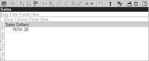
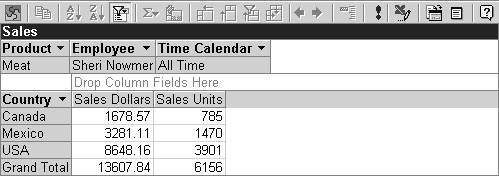
An MDX query statement uses several new terms. Seeing the terms in a familiar context will make them easier to learn and understand. Browsers such as the Office PivotTable list use MDX query statements to populate a report. You can use the Office PivotTable list to learn MDX terminology. The initial report in the Chapter 7 HTML file shows only a single cell showing the total value for the Sales Dollars measure. The grand total is a single value from the cube. To retrieve this value, Analysis Services used the default member for each dimension.

1.	In the Web browser, click the Field List toolbar button. Drag the Product, State, Employee, and Time Calendar dimensions from the PivotTable Field List window to the filter area of the report. Each dimension displays the default member in the filter area, and the total value never changes as you add the dimensions. (Since the Time Fiscal and Time Calendar dimensions are really hierarchies of the same dimension, you can include only one in the report at a time. The report still uses the default member of the unused dimension.) [View full size image] The default member allows a query to ignore some of the dimensions in a cube. If a dimension does not appear on the filter axis, it always uses the default member. If a dimension does appear on the filter axis, it can either use the default member or a different member. Putting a dimension on the filter area of a report overrides the default member for that dimension.
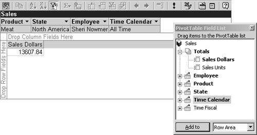
2.	Click the arrow next to the Product dimension list, select the Meat check box, and click OK to show only the total for meat. [View full size image] If you use nothing but the filter area, you create a report that displays only a single value, which is rarely useful. The row and column axes of a report allow you to display more than one member from a dimension. More than one member from a single dimension is called a set.
3.	Drag the State dimension to the row axis. The three countries—plus the total—appear. The row axis now displays a set that contains four positions. Each position in the set corresponds to a member from the State dimension. [View full size image]
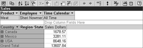
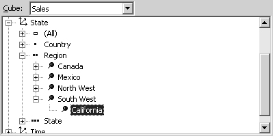
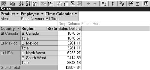
4.	Click the Country level label, and click the Expand toolbar button. [View full size image] The regions appear. The row axis now displays a set that contains eight positions. Even though the labels are split into two columns—to show the levels of the dimension—each position in the set still contains only a single member from the State dimension.
5.	Drag the Sales Units measure to the data area. The column axis now displays a set that contains two positions, each of which corresponds to a single member from the Measures dimension.
6.	For each cell value you see in the report, you can determine a complete tuple that includes one member from each dimension in the cube. For the cell in the Sales Dollars column with the value 6233.27, the Product dimension contributes Meat, the Employee Dimension contributes Sheri Nowmer, the Time Calendar dimension contributes All Time, and the State dimension contributes North West. Every value in an MDX report requires a single member from each dimension. The filter axis can include only a single member for any one dimension. The row and column axes can include only sets, which include multiple values from a single dimension. It’s not unusual for a cube to contain at least six or seven dimensions. Not counting the filter axis, a report based on an OLAP cube typically contains only two axes—columns and rows. Often, it’s useful to combine multiple dimensions from the cube onto a single axis of the report.
7.	In the PivotTable List document, drag the Region and State level headings away from the row area, leaving only the countries and Grand Total on the axis.
8.	Drag the Product level from the filter area to the row area, to the left of the State level. Drag the Subcategory and Product Name labels away from the report. Select the Category label, and click the Expand toolbar button. The report now shows both categories and countries on the row axis. The row axis still contains a set—a set with 13 positions. But each position within the set now contains a two-member tuple—a coordinate from more than one dimension. Note Technically, a set always contains tuples. Even when there is only one dimension on an axis, the set consists of single-member tuples.
9.	Drag the Time Calendar dimension from the filter area to the row area, to the left of the Category label. Drag the Calendar Quarter and Calendar Month labels away from the report. Then select the Calendar Year label, and click Expand. The report now shows years, categories, and countries on the row axis. The row axis still contains a set—now a set with 17 positions. But each position in the set now contains a three-member tuple. A tuple is a way to specify coordinates from more than one dimension on a single axis. The filter axis can contain only a single tuple. Row and column axes can each contain a set of tuples. The bottom line remains: for each value in the report, there’s a single member from each dimension that contributed to the complete coordinate for that cell in the cube. The member for a dimension can come from any of the axes—and more than one dimension can be represented on a single axis. Any dimension not found on the column, row, or filter axis uses the default member.

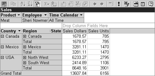
Use the MDX Sample Application

Analysis Services comes with the MDX Sample application. The application allows you to type an MDX statement, run it, and see the results in a grid. The MDX Sample application includes a metadata pane, which allows you to browse the hierarchies and members of a cube, inserting dimension, level, and member names into the MDX expression. The application also comes with complete source files for the Microsoft Visual Basic project used to create it. If you’re a programmer of Visual Basic, you can customize or add enhancements to the application. Some of the controls in the MDX Sample application are similar to those in the Calculated Member Builder. In this section, you’ll take a few minutes to explore the interface.

1.	Launch the MDX Sample application, which is on the Analysis Services menu along with Analysis Manager. Click OK to connect to the server. Click the New Query File toolbar button to create a new query file. A query file can contain multiple queries.
2.	In the toolbar, select Chapter 7 as the database name. Then, in the Cube drop-down list box, select Sales as the cube name. [View full size image] The MDX Sample application window is divided into three vertical panes. The top pane is the query pane, where you build an MDX query statement. The middle pane is the metadata pane, where you inspect information in a selected cube. The bottom pane is the results pane, which shows the output of an MDX query. Across the top of the application are a menu bar and a toolbar. Once you select a cube, the Metadata tree—the leftmost section of the metadata pane—displays the cube name as the top-level parent, plus the names of all the dimensions in the cube. The Metadata tree is equivalent to the Data tree in the Calculated Member Builder. The cube name has a cube icon to its left, and each dimension name has a triple-arrow icon to its left. Unlike the icons in Analysis Manager, the icons in the metadata view do not vary between different types of dimensions. The Metadata tree also displays members, but members often appear multiple times in the tree. Taking a close look at the metadata window can help you avoid confusion and get the most benefit from the MDX Sample application.
3.	Expand the State dimension. You see one entry for each level in the dimension, including the All level. The All level has a small rectangular icon to the left of the level name. Every other level has a dot-cluster icon. The number of dots represents the level’s depth in the hierarchy.
4.	Expand the State level. You see one entry for each member in the level. Each member name has a lollipop icon to its left. (It’s probably supposed to be a magnifying glass, but thinking of it as a lollipop is more vivid.)
5.	Collapse the State dimension, and then expand the Time dimension. You see two stair-step icons, one for the Calendar hierarchy and one for the Fiscal hierarchy. Then expand the Calendar hierarchy to see the level names. Note Each item in the Metadata tree is a cube, a dimension, a hierarchy, a level, or a member. These are all entities that exist within an OLAP database. That contrasts with sets and tuples, which exist only in an MDX expression. In other words, there are no sets or tuples in an OLAP database, just cubes, dimensions, hierarchies, levels, and members. For your convenience, the Metadata tree usually adds each member node to multiple locations in the tree. Specifically, in addition to adding a member node below the level at which it belongs—as with the State level—the Metadata tree also adds the same member as a child of its parent member. Some people find this redundancy confusing at first, but once you understand how the Metadata tree works, it really is convenient.
6.	In the State dimension, expand the Region level and the South West member. The California member appears below South West. California is the child—the only child—of the South West member. The California member appears both in the State level and also as a child of the South West member.
7.	Expand the Country level, the USA member, and the South West member. You see the California member once again—this time as a “grandchild” of USA. The California member is still on the State level. The highest member in an ancestry tree belongs to the level name just above it. For example, USA belongs to the Country level. For each degree of indentation, the members belong to a level one lower in the cube. For example, South West belongs to the Region level—even though the member node can appear under the Country level. Likewise, California belongs to the State level—even though the member node can appear under the Country or Region levels as well as the State level. You can double-click any node to have the fully qualified name of the item appear in the query pane. You can also drag a node to the query pane, in case you didn’t put the insertion point in the proper place.
8.	Double-click the California member. The full name of the member appears in the query pane. Double-clicking a leaf-level member in the tree view does not move the member into the query pane. You can, however, drag a leaf-level member into the query pane or select the level name and double-click a member from the member list.

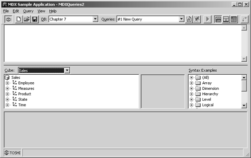
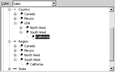
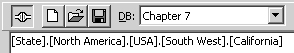
In the Metadata tree, when you select either a level or a member that has children, the members appear in the list to the right of the metadata pane. You can double-click or drag members from the member list to add them to the query pane.