

chapter 2
Basic Developments
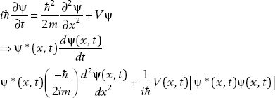
In quantum mechanics, information about the state of a particle is described by a wavefunction. This function is usually denoted by ψ(x, t). The equation that describes its time evolution is called the Schrödinger equation.
CHAPTER OBJECTIVES
In this chapter you will
• Learn about the Schrödinger equation and wavefunctions
• Explore energy states of particles
• Understand the probability interpretation of quantum mechanics
• Find out how to normalize wavefunctions
The Schrödinger Equation
The behavior of a particle of mass m subject to a potential V(x, t) is described by the following partial differential equation:
where ψ(x, t) is called the wavefunction. The wavefunction contains information about where the particle is located, since its square is a probability density. Specifically, the integral of the square of the wavefunction gives the probability of finding the particle at position x at time t—That is, if P is the probability of finding the particle between a and b, then
A wavefunction must be “well behaved.” In other words, it should be defined and continuous everywhere. In addition it must be square-integrable, meaning
SUMMARY: Properties of a Valid Wavefunction
A wavefunction ψ must be
• Single-valued
• Continuous
• Differentiable
• Square-integrable
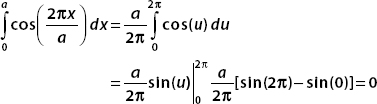
Let two functions ψ and Φ be defined for 0 ≤ x < ∞. Explain why ψ(x) = x cannot be a wavefunction but  could be a valid wavefunction.
Both functions are continuous and defined on the interval of interest. They are both single-valued and differentiable. However, consider the integral of x:
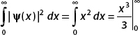
Given that ψ(x) = x is not square-integrable over this range, it cannot be a valid wavefunction. On the other hand,
Therefore, is square-integrable, so we can say it’s well behaved over the interval of interest. This makes it a valid candidate wavefunction. Figure 2-1 shows that this function is smooth and decays rather quickly.
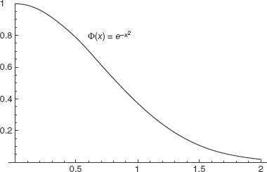
FIGURE 2-1
DEFINITION: The Probability Interpretation of the Wavefunction
At time t, the probability of finding the particle within the interval between x and x + dx is given by the square of the wavefunction. Calling this probability dP (x, t), we write
The square is given by |ψ(x,t)|2 because, in general, the wavefunction can be complex. In these dimensions, the Schrödinger equation is readily generalized to
where ∇2 is the Laplacian operator, which can be written as
in cartesian coordinates. The probability of finding the particle then becomes the probability of locating it within a volume d 3r = dx dy dz.
For the time being we will focus on one-dimensional situations. In most cases of interest, the potential V is a function of position only, and so we can write
The Schrödinger equation has two important properties:
1. The equation is linear and homogeneous.
2. The equation is first-order with respect to time, meaning that the state of a system at some initial time t0 determines its behavior for all future times.
An important consequence of the first property is that the superposition principle holds.
This means that if ψ1(x, t), ψ2(x, t), …, ψn(x, t) are solutions of the Schrödinger equation, then the linear combination of these functions
is also a solution. We will see that this superposition property is of critical importance in quantum theory.
Solutions to the Schrödinger equation when a particle is subject to a time-independent potential V(x) can be found by using separation of variables. This is done by writing the wavefunction in the form
Since the Schrödinger equation is first-order in the time derivative, this leads to a simple solution to the time-dependent part of the wavefunction.
where E is the energy.
Consider a particle trapped in a well with potential given by

Show that ψ(x, t) = A sin(kx) eiEt/ solves the Schrödinger equation provided that
The potential is infinite at x = 0 and a; therefore, the particle can never be found outside of this range. So we only need to consider the Schrödinger equation inside the well, where V = 0. With this condition the Schrödinger equation takes the form
Setting ψ(x, t) = A sin(kx) e−iEt/, we consider the left side of the Schrödinger equation first:
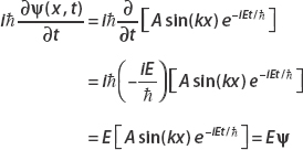
Now consider the derivative with respect to x:
Using
we equate both terms, finding that
And so we conclude that the Schrödinger equation is satisfied if
Solving the Schrödinger Equation
We have seen that when the potential is time-independent, the solution to the Schrödinger equation is given by
The spatial part of the wavefunction Φ(x) satisfies the time-independent Schrödinger equation.
DEFINITION: The Time-Independent Schrödinger Equation
Let 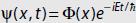 be a solution to the Schrödinger equation with time-independent potential V = V(x). The spatial part of the wavefunction Φ(x) satisfies
where E is the energy of the particle. This equation is known as the time-independent Schrödinger equation.
Solutions that can be written as  are called stationary.
DEFINITION: Stationary State
A solution to the Schrödinger equation is called stationary because the probability density does not depend on time:
We now consider an example where we are given the wavefunction. If we know the form of the wavefunction, it is easy to find the potential so that the Schrödinger equation is satisfied.
Suppose ψ(x,t) = A(x – x3)e−iEt/. Find V(x) such that the Schrödinger equation is satisfied.
The wavefunction is written as a product:
Therefore it is not necessary to work with the full Schrödinger equation. Recalling the time-independent Schrödinger equation
we set Φ(x) = A(x – x3) and solve to find V. The right-hand side is simply
To find the form of the left side of the equation, we begin by computing the first derivative:
Putting this in the left side of the time-independent Schrödinger equation and equating this to EA (x − x3) give
Now subtract (2/2m)6Ax from both sides:
Dividing both sides by A(x – x3) gives us the potential
Most of the time, we are given a specific potential and asked to find the form of the wavefunction. In many cases this involves solving a boundary value problem. A wavefunction must be continuous and defined everywhere, so the wavefunction must match up at boundaries. The process of applying boundary conditions to find a solution to a differential equation is no doubt familiar. We show how this is done in quantum mechanics with a problem we introduced earlier, the infinite square well.
Solve the Schrödinger equation for this potential.
Inside the box, the potential V is zero, and so the Schrödinger equation takes the form
We already showed that the solution to this problem is separable. Therefore, we take
The time-independent equation with zero potential is
Dividing through by − /2m and moving all terms to one side, we have
If we set k2 = 2mE/2, we obtain
The solution of this equation is
To determine the constants A and B, we apply the boundary conditions. Since the potential is infinite at x = 0 and x = a, the wavefunction is zero outside of the well. A wavefunction must be defined and continuous every-where. This tells us that any solution we find inside the well must match up to what is outside at the boundaries.
At x = 0, the solution becomes
The requirement that ψ(0) = 0 tells us that
The wavefunction must also vanish at the other end of the well. This means we must also enforce the condition ψ(a) = 0:
This can only be true if A = 0 or if sin(ka) = 0. The first possibility is not of any interest; a wavefunction that is zero everywhere is the same as saying there is no particle present. So we pursue the latter possibility. Now sin(ka) = 0 if
where n = 1, 2, … So we set k = nπ/a, and the wavefunction can be written as
The constant A is determined by normalizing the wavefunction, a technique we discuss in the next section. For now we will just carry it along.
Earlier, we defined the constant k in terms of the particle’s energy E. Let’s use this definition to write down the form of the energy in terms of nπ/a:
If n = 0, the wavefunction will vanish, indicating there is no particle in the well. Therefore the lowest possible energy a particle can have is found by setting n = 1:
The lowest energy is called the ground state energy.
DEFINITION: Ground State
The ground state is the state with the lowest energy a system can assume.
For the infinite square well, all other energies are given in terms of integer multiples of the ground state energy. Figures 2-2, 2-3, and 2-4 are sample plots of the first three wavefunctions with a = 3.
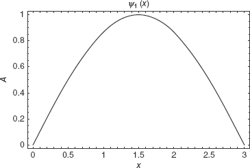
FIGURE 2-2
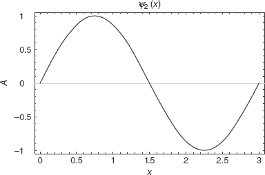
FIGURE 2-3
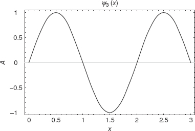
FIGURE 2-4
As you might have guessed, in general En = n2E1.
The square of the wavefunction gives the probability density. We can say that the intensity of the wave at a given point is proportional to the likelihood of finding the particle there. Figure 2-5 is a plot of |ψ3(x)|2.
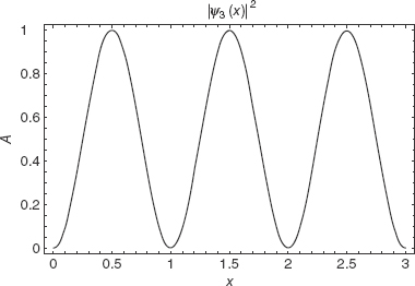
FIGURE 2-5
From the plot we can surmise that the particle is most likely to be found at x = 0.5, 1.5, and 2.5, but is not ever going to be found at x = 1, x = 2, or the boundaries.
The concept of energy levels is unfamiliar from our study of classical mechanics, where basically a particle can have any energy in a continuous fashion. In quantum mechanics, the ground state is the lowest possible energy, and often the lowest energy state is not zero energy.
The Probability Interpretation and Normalization
The probability interpretation tells us that |ψ(x, t)|2 dx gives the probability for finding the particle between x and x + dx. To find the probability that a particle is located within a given region, we integrate.
DEFINITION: Finding the Probability That a Particle Is Located in the Region a ≤ x ≤ b
The probability p that a particle is located within a ≤ x ≤ b is
It is common to denote a probability density |ψ(x, t)|2 as ρ(x, t).
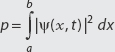
Suppose that a certain probability distribution is given by  for 1 ≤ x ≤ 3. Find the probability that 5/2 ≤ x ≤ 3.
If this were a wavefunction, there would be about a 5.5 percent chance of finding the particle between 5/2 ≤ x ≤ 3.
The total probability for any distribution must sum to unity. If the probability distribution is discrete with n individual probabilities pi, this means that
For a continuous probability distribution p(x), the fact that probabilities must sum to unity means that
In quantum mechanics, this condition means that the particle is located some-where in space with certainty.
As we saw in the solution to the square well, a wavefunction that solves the Schrödinger equation is determined up to an unknown constant. In that case, the constant is called the normalization constant, and we find the value of that constant by normalizing the wavefunction.
DEFINITION: Normalizing the Wavefunction
When a wavefunction that solves the Schrödinger equation is multiplied by an undetermined constant A, we normalize the wavefunction by solving:
The normalized wavefunction is then Aψ(x, t).
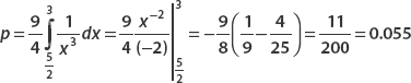
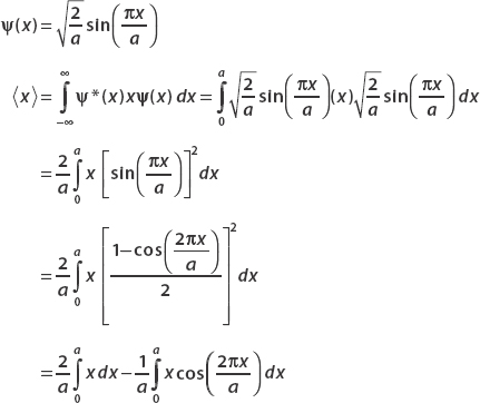
The wavefunction for a particle confined to 0 ≤ x ≤ a in the ground state was found to be
where A is the normalization constant. Find A and determine the probability that the particle is found in the interval  .
.
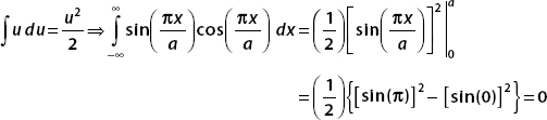
Normalization means that
The wavefunction is zero outside of the interval 0 ≤ x ≤ a; therefore we only need to consider
We use the trigometric identity sin2 u = (1 – cos 2u)/2 to rewrite the integrand:
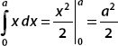
The first term can be integrated immediately:
For the second term, let
and
And so, only the first term contributes, and we have
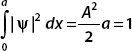
Solving for the normalization constant A, we find
and the normalized wavefunction is
The probability that the particle is found in the interval  is given by
Find A and B so that
is normalized.
Using 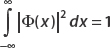 , we obtain
As long as 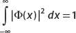 is satisfied, we are free to arbitrarily choose one of the constants as long as it’s not zero. So we set B = 1:
Normalize the wavefunction
We start by finding the square of the wavefunction:
To compute  , we will need two integrals, which can be found in integration tables:
We begin by using the second integral:
where the first term is to be evaluated at ±∞. Consider the limit as x → ∞:
where L’Hôpital’s rule was used. Similarly, for the lower limit we find
So we can discard the first term altogether. Now we can use 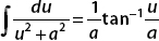 for the remaining piece.
Again we recall that the normalization condition is
Therefore, setting our result equal to 1, we find that
And so the normalized wavefunction is
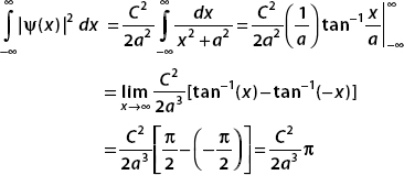
In the next examples, we consider the normalization of some gaussian functions. We will use three frequently seen integrals:
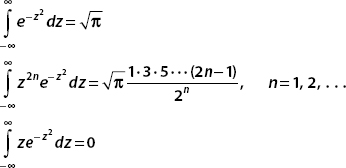
We also introduce the error function:
Find A such that ψ(x) is normalized. The constants λ and x0 are real.
For normalization, we set 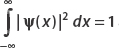 and then solve for A.
We can perform this integral by using the substitution  . Then
Using  , we find that
  .
.
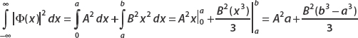
(a) Write the normalization condition for A1 and A2.
(b) Normalize ψ(x) for A1 = A2 and a = 32, b = 8.
(c) Find the probability that the particle is found in the region 0 < x < 32.
(a)
The normalization condition is  . Now since
  , the middle term vanishes, and we have
Looking at the first term, we use the substitution technique from calculus to get it in the form
Let z2 = (2x2)/a. Then  . Therefore we can write the integral as
Turning to the second term, we again use a substitution. This time we want the form
As before, let z2 = (2x2)/b; then 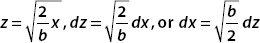 . Also
So we can rewrite the second integral in the following way:
Using  for n = 1, we obtain
Putting these results together, we obtain the normalization condition:
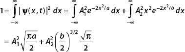
(b) Now let A1 = A2 and a = 32, b = 8. The normalization condition becomes
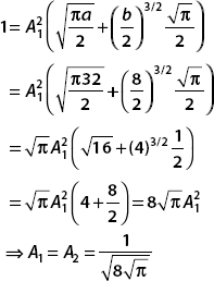
And so, the normalized wavefunction in this case is
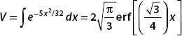
(c) The probability that the particle is found in the interval 0 < x < 32 is
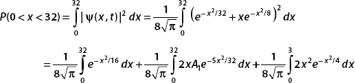
To perform these integrals, we consider the error function. This is given by
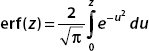
We use substitution techniques to put the integrals into this form. It turns out that erf(32) ≈ 1.
For the second integral, we use integration by parts. Let u = x, then du = dx. If dV = e−5x2/32, then
Now let a dummy variable  . This allows us to put this in the form of erf(32):
And so, with u = x, using integration by parts, 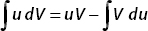 , we obtain
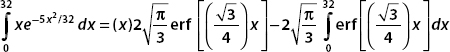
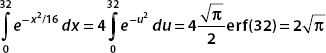
These terms can be evaluated numerically. The integration is between the limits x = 0 and x = 32. Now erf(0) = 0, and so the first term is
The second term is
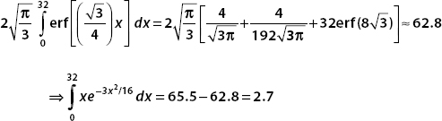
Now the final term, which we evaluate numerically, is
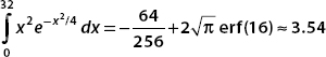
Pulling all these results together, we see the probability that the particle is found in the interval 0 < x < 32 is
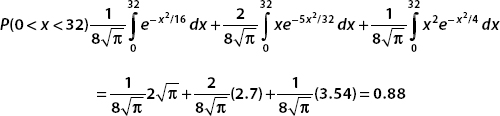
Conclusion: For 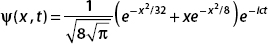 defined for −∞< x <∞, there is an 88% chance that we will find the particle in the interval 0 < x < 32.
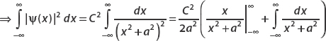
Let ψ(x) = Ae−|x|/2aei(x−x0). Find the constant A by normalizing the wavefunction.
First we compute
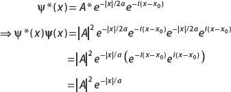
To integrate e−x/a, think about the fact that it’s defined in terms of the absolute value function. For |x| < 0, this term is ex/a, while for x > 0 it’s e−x/a. So we split the integral into two parts:
Let’s look at the first term (the second can be calculated in the same way modulo a minus sign). Let u = x/a, then du = dx/a. And so
Application of the same technique to the second term also gives a, and so
Using the normalization condition
we obtain
The normalized wavefunction is then
Expansion of the Wavefunction and Finding Coefficients
Earlier we noted that the superposition principle holds. Consider the superposition of stationary states ψ1(x, t), ψ2(x, t),…, ψn(x, t) which are solutions of the Schrödinger equation for a given potential V. Since these are stationary states, they can be written as
At t = 0, any wavefunction ψ can be written as a linear combination of these states:
If we set E = ω, the time evolution of this state is then
Since any function ψ can be expanded in terms of the Φn, we say that the Φn are a set of basis functions. This is analogous to the way a vector can be expanded in terms of the basis vectors {i, j, k}. Sometimes we say that the set Φn is complete—this is another way of saying that any wavefunction can be expressed as a linear combination of them.
To understand the mathematical behavior of wavefunctions, use your knowledge of freshman physics. Wavefunctions behave just as ordinary vectors in a mathematical sense. Normalization is akin to making a unit vector.
DEFINITION: State Collapse
Suppose that a state ψ is given by
A measurement of the energy is made and found to be Ei = ωi. The state of the system immediately after measurement is Φi (x), that is,
A second measurement of the energy conducted immediately after the first will find Ei = ωi with certainty. However, if the system is left alone, the wavefunction will “spread out” as dictated by the time evolution of the Schrödinger equation and will again become a superposition of states.
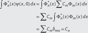
To find the constants Cn in the expansion of ψ, we use the inner product.
DEFINITION: Inner Product
The inner product of two wavefunctions ψ(x) and Φ(x) is defined by
The square of (Φ, ψ) tells us the probability that a measurement will find the system in state Φ(x), given that it is originally in the state ψ(x).
Basis states are orthogonal. That is,
A shorthand for this type of relationship is provided by the Kronecker delta function:
This allows us to write
The fact that basis states are orthogonal allows us to calculate the expansion coefficients using inner products.
DEFINITION: Calculating a Coefficient of Expansion
If a state ψ(x, 0) is written as a summation of basis functions Φn (x), we find the nth coefficient of the expansion Cn by computing the inner product of Φn (x) with ψ(x, 0). That is,
Notice that
DEFINITION: The Meaning of the Expansion Coefficient
If a state is written as 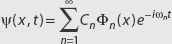 , the modulus squared of the expansion coefficient Cn is the probability of finding the system in state Φn (x), that is,
Probability system is in state Φn(x) = |Cn|2
In other words, if a state 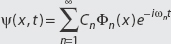 and we measure the energy,
what is the probability we find En = ωn? The answer is |Cn|2. Since the coefficients Cn define probabilities, it must be true that
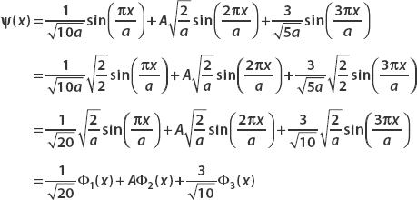
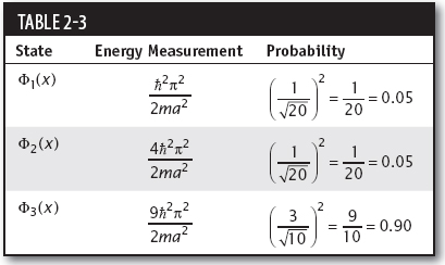
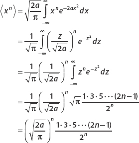
A particle of mass m is trapped in a one-dimensional box of width a. The wavefunction is known to be
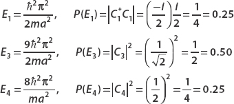
If the energy is measured, what are the possible results and what is the probability of obtaining each result? What is the most probable energy for this state?
We begin by recalling that the nth excited state of a particle in a one-dimensional box is described by the wavefunction
Table 2-1 gives the first few wavefunctions and their associated energies.
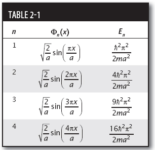
Noting that all the Φn multiplied by the constant  , we rewrite the wavefunction as given so that all three terms look this way:
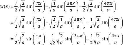
Now we compare each term to the table, allowing us to write this as
Since the wavefunction is written in the form 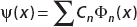 , we see that the coefficients of the expansion are as shown in Table 2-2.
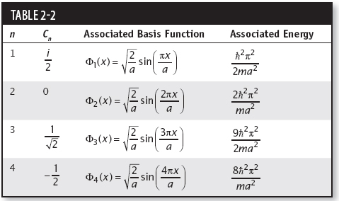
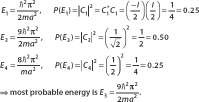
Since C2 is not present in the expansion, there is no chance of seeing the energy E = n22π2/2ma2. The square of the other coefficient terms gives the probability of measuring each energy. So the possible energies that can be measured with their respective probabilities are
A particle in a one-dimensional box 0 ≤ x ≤ a is in the state
(a) Find A so that ψ(x) is normalized.
(b) What are the possible results of measurements of the energy, and what are the respective probabilities of obtaining each result?
(c) The energy is measured and found to be (2π22)/(ma2). What is the state of the system immediately after measurement?
(a) The basis functions for a one-dimensional box are
First we manipulate ψ(x) so we can write each term with the coefficient  .
.
Now we compute the inner product (ψ(x),ψ(x)). We must have (ψ(x), ψ(x)) = 1 for the state to be normalized. Since Φm(x)Φn(x)dx = δmn, we can drop all terms where m ≠n:
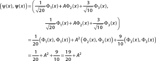
Setting this equal to 1 and subtracting 19/20 from both sides, we have
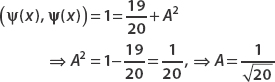
So the normalized wavefunction is
(b) In the one-dimensional box or infinite square well, the possible result of a measurement of energy for Φn(x) is
To determine the possible results of a measurement of the energy for a wavefunction expanded in basis states of the Hamiltonian, we look at each state in the expansion. If the wavefunction is normalized, the squared modulus of the coefficient multiplying each state gives the probability of obtaining the given measurement. Looking at ψ(x), we see that the possible results of a measurement of the energy and their probabilities are as shown in Table 2-3.
(c) If the energy is measured and found to be (2π22)/(ma2) = (4π22)/(2ma2), the state of the system immediately after measurement is
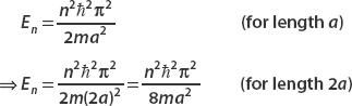
A particle of mass m is confined in a one-dimensional box with dimensions 0 ≤ x ≤ a and is known to be in the second excited state (n = 3). Suddenly the width of the box is doubled (a → 2a), without disturbing the state of the particle. If a measurement of the energy is found, find the probabilities that we find the system in the ground state and the first excited state.
The stationary state for a particle in a box of length a is
The second excited state wavefunction for a particle in a one-dimensional box is n = 3. So the wavefunction is
Now let’s consider a box of length 2a. Labeling these states by Φn(x), we just let a → 2a:
The energy of each state is also found by letting a → 2a:
Given that the system is in the state 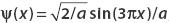 , we use the inner product (Φn, ψ) to find the probability that the particle is found in state Φn(x) when a measurement is made.
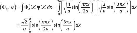
To perform this integral, we use the trig identity
Putting this result into the integral gives
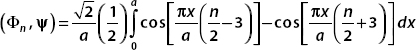
Each term is easily evaluated with a substitution. We set u = (πx/a)[(n/2) − 3] in the first integral and u = (πx/a)[(n/2) + 3] in the second. Therefore,
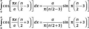
If n is even, then we get the sine of an integral multiple of π, and both terms are zero. Putting all these results together, we have
The first excited state has n = 2. Since
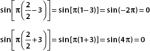
then (Φ2, ψ) = 0, and so the probability of finding the system in the first excited state vanishes. For the ground state n = 1, and we have
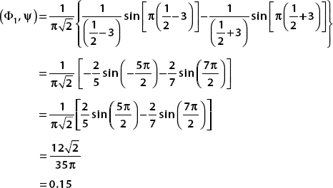
The probability is found by squaring this number. So the probability of finding the system in the ground state of the newly widened box is
P(n = 1) = (0.15)2 = 0.024
The Phase of a Wavefunction
A phase factor is some function of the form eiθ that multiplies a wavefunction. If the phase is an overall multiplicative factor, it is called a global phase. Suppose we have two wavefunctions:
Notice that
Since both states give the same physical predictions (i.e., they predict the same probabilities of measurement in terms of the modulus square of the wavefunction), we say they are physically equivalent. We can go so far as to say that they are the same state.
Now we consider a type of phase called relative phase. Suppose that we expand a wavefunction in terms of normalized basis states. For simplicity, we consider
Then
In this case,  , and therefore these wavefunctions do not represent the same physical state. Each wavefunction will give rise to different probabilities for the results of physical measurements. We summarize these results.
DEFINITION: Global Phase
A global phase factor in the form of some function eiθ that is an overall multiplicative constant for a wavefunction has no physical significance—ψ(x) and eiθψ(x) represent the same physical state.
DEFINITION: Local Phase
A relative phase factor in the form of a term eiθ that multiplies an expansion coefficient in  does change physical predictions.
and
do not represent the same state.
Operators in Quantum Mechanics
An operator is a mathematical instruction to do something to the function that follows. The result is a new function. A simple operator could be to just take the derivative of a function. Suppose we call this operator D. Then
Or in shorthand we just write
Consider another operator, which we call X; then multiply a function by x:
Operators are often represented by capital letters, sometimes using a caret, for example,  . If given scalars α and β and functions ψ(x) and x that an operator A satisfies
we say that operator A is linear. If the action of an operator on a function Φ(x) is to multiply that function by some constant
we say that the constant A is an eigenvalue of the operator A, and we call Φ(x) an eigenfunction of A.
Two operators are of fundamental importance in quantum mechanics. We have already seen one of them. The position operator acts on a wavefunction by multiplying it by the coordinate:
In three dimensions, we also have operators Y and Z:
In quantum mechanics, we also have a momentum operator. The momentum operator is given in terms of differentiation with respect to the position coordinate:
Therefore the momentum operator is  . If we are working in three dimensions, we also have momentum operators for the other coordinates:

The expectation value or mean of an operator A with respect to the wavefunction ψ(x) is
The mean value of an operator is not necessarily a value that can actually be measured. So it may not turn out to be equal to one of the eigenvalues of A.
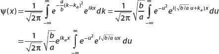
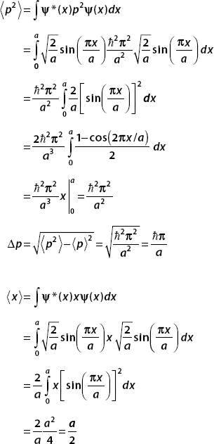
A particle of mass m in a one-dimensional box were 0 ≤ x ≤ a, is in the ground state. Find  and
and  .
.
The wavefunction is
Integrating the first term yields
To calculate , we write p as a derivative operator:
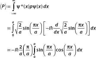
You may already know this integral is zero, but we can calculate it easily, so we proceed.
Let  , then
 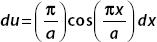 . this gives
And so, for the ground state of the particle in a box, we have found
Let
So the expectation value of x n is given by
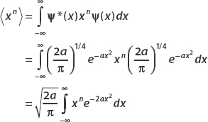
We can do this integral, recalling that
Looking at the integral for  , let
, let  ; then
  . For even n = 2, 4, 6, 8, … we obtain
Earlier we noted that
In fact,
for any odd m; therefore  if n is odd.
If a normalized wavefunction is expanded in a basis with known expansion coefficients, we can use this expansion to calculate mean values. Specifically, if a wavefunction has been expanded as
and the basis functions Φn(x) are eigenfunctions of operator A with eigenvalues an, then the mean of operator A can be found from
If the following relationship holds:
we say that the operator A is Hermitian. Hermitian operators, which have real eigenvalues, are fundamentally important in quantum mechanics. Quantities that can be measured experimentally, such as energy or momentum, are represented by Hermitian operators.
We can also calculate the mean of the square of an operator:
where A2 is the operator (A)(A). This leads us to a quantity known as the standard deviation or uncertainty in A:
This quantity measures the spread of values about the mean for A.
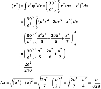
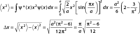
(a) Normalize the wavefunction.
(b) Find ,  , and Δx.
(a) The wavefunction is real. So ψ*ψ = ψ2 and we have
One very important operator that we will come across frequently is the Hamiltonian operator:
As you can see, this is just one side of the Schrödinger equation. Therefore H acting on a wavefunction gives
When the potential is time-independent and we have the time-independent Schrödinger equation, we arrive at an eigenvalue equation for H:
The eigenvalues E of the Hamiltonian are the energies of the system. Or you can say the allowed energies of the system are the eigenvalues of the Hamiltonian operator H. The average or mean energy of a system expanded in the basis states ϕn is found from
where pn is the probability that energy is measured.
Earlier we considered the following state for a particle trapped in a one-dimensional box:
What is the mean energy for this system?
The mean energy is
Note that the mean energy would never actually be measured for this system.
Is the momentum operator p Hermitian?
We need to show that
Using 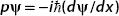 , we have
Recalling the formula for integration by parts,
We let
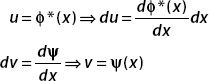
The wavefunction must vanish as x →±∞, and so the boundary term (uv = ϕ*(x)ψ(x)) vanishes. We are then left with
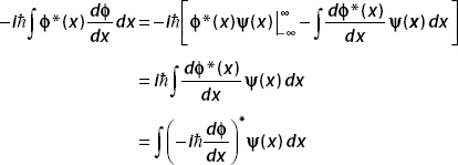
We have shown that 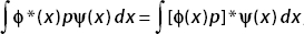 , therefore p is Hermitian.
Momentum and the Uncertainty Principle
The fact that momentum can be expressed as p = k allows us to define a “momentum space” wavefunction that is related to the position space wavefunction via the Fourier transform. A function f(x) and its Fourier transform F(k) are related via the relations
These relations can be expressed in terms of p with a position space wavefunction ψ(x) and momentum space wavefunction ϕ(p) as
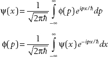
Parseval’s theorem tells us that
These relations tell us that ϕ(p), like ψ(x), represents a probability density. The function ϕ(p) gives us information about the probability of finding momentum in the interval a ≤ p ≤ b:
Parseval’s theorem tells us that if the wavefunction ψ(x) is normalized, then the momentum space wavefunction ϕ(p) is also normalized:
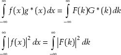
Suppose that
Find the momentum space wavefunction ϕ(p).
Figure 2-6, a plot, of the so-called sinc function, shows that the momentum space wavefunction, like the position space wavefunction in this case, is also localized.
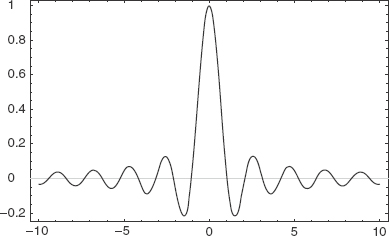
FIGURE 2-6
It is a fact of Fourier theory and wave mechanics that the spatial extension of the wave described by ψ(x) and the extension of the wavelength described by the Fourier transform ϕ(p) cannot be made arbitrarily small. This observation is described mathematically by the Heisenberg uncertainty principle:
Δx Δp ≥
Or, using p = k, Δx Δk ≥ 1.
Let
Use the Fourier transform to find ψ(x).
We can find the position space wavefunction from the relation
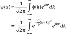
To perform this daunting integral, we resort to an integral table, where we find that
Examining the Fourier transform, we let
Then we have
This substitution gives us
Now we can make the following identifications with the result from the integral table:
And so the position space wavefunction is
A particle of mass m in a one-dimensional box is found to be in the ground state:
Find Δx Δp for this state.
Using p = id/dx, we have
and
We found in the example above that = 0 for this state.
Notice that  , and so Δx Δp > /2.
The Conservation of Probability
The probability density is defined as
We know that ψ(x,t) satisfies the Schrödinger equation. It is also true that ψ*(x,t) satisfies the Schrödinger equation. Let’s take the time derivative of the product:
Recalling the Schrödinger equation,
(2.1)
Taking the complex conjugate of the Schrödinger equation, we find the equation satisfied by ψ* (x, t):
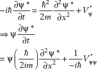
(2.2)
Now we add Eqs. (2.1) and (2.2). On the left side, we obtain
On the right side, we get
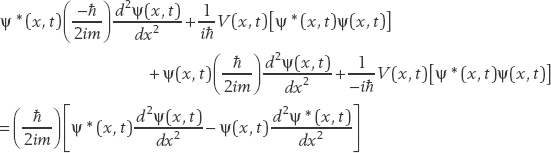
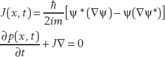
We use this result as the basis for a new function called the probability current j(x, t), which is defined as
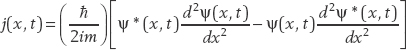
We see that the result on the right side is −∂j/∂x. Setting this equal to the result on the left-hand side, we obtain the continuity equation for probability:
In three dimensions, this generalizes to
Suppose that a particle of mass m in a one-dinensional box is described by the wavefunction
Find the probability current for this wavefunction.
By definition,
Now
and
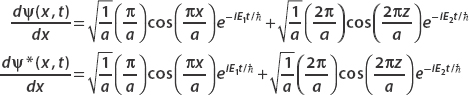
Algebra shows that
Using
we find that for this wavefunction
Summary
In this chapter we learned the basic fundamentals of quantum mechanics:
• Particle behavior is described by the Schrödinger equation.
• Wavefunctions that solve the Schrödinger equation obey the superposition principle.
• The probability interpretation tells us that the wavefunction represents the probability that a particle will have a given energy or be found in a certain location.
• A consequence of the probability interpretation is that wavefunctions must be normalized.
QUIZ
1. A. Set ψ(x, t) = ϕ(x)f (t) and then apply the Schrödinger equation to show that this leads to a solution of f(t) = e−iEt/.
B. For the equation  verify that the solution is
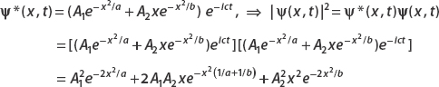
2. Let  defined for −∞ < x < ∞.
A. Show that 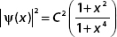 .
.
B. Normalize ψ and show that  .
.
C. Show that the probability that the particle is found in the interval 0 ≤ x ≤ 1 is 0.52.
3. Let a wavefunction be given by
A. Show that if ψ(x,t) is normalized, then  .
.
B. Show that the probability of finding the particle in the interval  .
.
4. For the wavefunction
Defined for −∞ < x < ∞, show that = 0 and = 9.
5. Suppose that a wavefunction is given by
Find Δx and Δp for this wavefunction.
6. Determine whether the operator X is Hermitian. What about iX? If it is not, why not?
7. Let  .
.
Find the probability current and check to see if the continuity equation is satisfied.
8. A particle in an infinite square well of dimensions 0 ≤ x ≤ a is in a state described by
A. Is ψ(x, t) normalized?
B. What values can be measured for the energy and with what probabilities?
C. Find and for this state. Do these quantities depend on time? If so, is it true that md/dt = ?
9. Explain why there is a correspondence between a physical wavefunction and a unit vector.
10. If  , how can you find the components of the wavefunction?
11. A vector is said to be positive semidefinite if  . Why do you think a wavefunction must be positive semidefinite?
12. What is the fundamental difference between the energy of a bound classical particle and the energy of a bound quantum mechanical particle?
..................Content has been hidden....................
You can't read the all page of ebook, please click here login for view all page.