

chapter 3
The Time-Independent Schrödinger Equation
For a particle of mass m in a potential V, the time-independent Schrödinger equation is written as
where E is the energy. The Hamiltonian operator is defined to be
Therefore the time-independent Schrödinger equation has the form of an eigenvalue equation
where the eigenvalues of H are the possible energies E of the system and the eigenfunctions of H are wavefunctions. We proceed to solve this equation under different conditions.
CHAPTER OBJECTIVES
In this chapter you will
• Learn how to apply the Schrödinger equation to the free particle
• Solve the Schrödinger equation for bound states
• Solve the Schrödinger equation when a particle encounters a barrier
The Free Particle
When V = 0, we obtain the solution for a free particle. The Schrödinger equation becomes
Moving all terms to the left side gives
Now multiply through by −2m/ 2:
2:
Now define the wavenumber k, using the relationship
We use the wavenumber to define the energy and momentum of the free particle.
DEFINITION: Kinetic Energy and Momentum of a Free Particle
Defined in terms of the wavenumber, the kinetic energy of a free particle is
The momentum of a free particle is
The wavenumber k can assume any value. Written in terms of a wavenumber, the equation becomes
There are two possible solutions to this equation:
As an example, we try the first solution. The first derivative gives
For the second derivative, we find
Therefore it is clear that
and the equation is satisfied. You can try this for the other solution and get the same result. We have found two solutions that solve the equation and correspond to the same energy E. This situation is known as degeneracy.
DEFINITION: Degeneracy
Degeneracy results when two (or more) different solutions to an eigenvalue equation correspond to the same eigenvalue.
For the current example, this means that a measurement of the energy that finds
cannot determine if the particle is in state ψ1 or state ψ2. To distinguish between the two states, an additional measurement is necessary. This requirement can be accommodated with the momentum operator. Recalling that the momentum operator is represented by
we apply the momentum operator to the two wavefunctions that solve the free particle equation and find
which implies that Ae ikx is an eigenfunction of the momentum operator with eigenvalue k. This wavefunction describes a particle moving to the right along the x axis.
The same procedure applied to ψ2(x) shows that Ae -ikx is an eigenfunction of the momentum operator with eigenvalue − k. This wavefunction describes a particle moving to the left along the x axis.
So we see that these eigenfunctions are simultaneous eigenfunctions of energy and momentum.
In Chap. 2, it was emphasized that normalization is a critical property that a wavefunction must have. The free particle solution cannot be normalized. In either case,
So far, we can make the following observations about the free particle solution:
1. The free particle solutions, like those for the infinite square well, are given in terms of Ae ikx. This is not surprising because inside the infinite square well, the potential is zero.
2. The boundary conditions of the square well put limits on the values that k could assume. In this case there are no boundary conditions, and therefore k can assume any value.
3. The wavefunction is not normalizable.
In deriving the free particle wavefunction, we solved the time-independent Schrödinger equation. This is an implicit way of stating that we are assuming separable solutions. Since we have found such solutions and they are not normalizable, this means that a separable solution, which represent stationary states of definite energy, is not possible for a free particle. The way to get around this problem is to take advantage of the linearity of the Schrödinger equation and form a superposition of solutions together (by adding values of k) to form a new solution. We can always write the exponential solutions in terms of sine and cosine functions. So let’s consider a wavefunction of the form
and see what happens as we add various values of k. Figures 3-1 and 3-2 are plots of cos(2x), cos(4x), and cos(6x).

FIGURE 3-1

FIGURE 3-2
If we add these waves, the waves add in some places and cancel in others, and we start to get a localized waveform in Fig. 3-3.

FIGURE 3-3
Now look what happens when we add waves with many values of k (see Fig 3-4). The wavepacket becomes more and more localized.
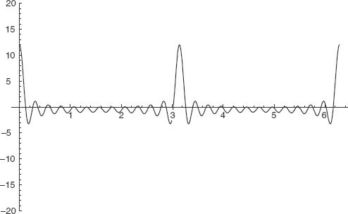
FIGURE 3-4
For the free particle, this type of wave addition process gives us a localized wavepacket.
Let ψ1(x) = cos(2x) and ψ2(x)=cos(10x). Describe and plot the wavepacket formed by the superposition of these two waves.
To form the wavepacket, we use the trig identity:

The plot of ψ2(x) is shown in Fig. 3-5.
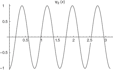
FIGURE 3-5
The plot of ψ1(x) is shown in Fig. 3-6.
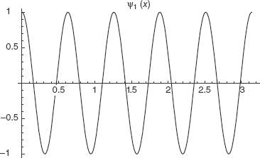
FIGURE 3-6
Finally we plot ψ1(x) + ψ2(x). Notice how it shows hints of attaining a localized waveform in Fig. 3-7.
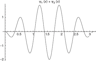
FIGURE 3-7
The way to construct a wavepacket by adding a large number of values of k is to integrate. In other words, wavepackets are constructed by using the Fourier transform.
Following the procedure described in Chap. 2, we append onto the time dependence of the wavefunction by writing
Using  , we can write
The wavepacket is formed by multiplying a momentum space wavefunction ϕ(k) and adding over values of k, which means we integrate:

DEFINITION: Dispersion Relation
The dispersion relation is a functional relationship that defines angular frequency ω in terms of the wavenumber k, that is, ω = ω (k). The dispersion relation can be used to find the phase velocity and group velocity for a wavepacket.
Phase velocity is given by  , while group velocity
  . In the case of the free particle, we have
The Einstein-Planck relations tell us that E = ω; setting these equal gives
Solving for ω yields
Therefore the phase velocity and group velocity are
Notice that the phase velocity is one-half of what the velocity of a classical particle would be, while the group velocity gives the correct classical velocity. In general, these expressions will be more complicated. We have used the energy relation for a single free particle solution to the Schrödinger equation.
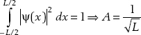
Let’s now review the situation where the particle is limited to a fixed region of space and see how this forces a quantization of k (and therefore the energy). Another way to obtain a normalizable solution to the free particle wavefunction is to impose periodic boundary conditions. If the particle is constrained between ±L/2, then normalization becomes

This leads to a solution for A:
The normalized wavefunction is
Periodic boundary conditions, while requiring that the particle be confined between ±L/2, are manifested by requiring that
This condition leads to
which means that
The left side is purely real and the right side has an imaginary term, so that the imaginary piece must be zero. This can be true if
where n = 0, ±1, ±2, ±3,. … The wavenumber k, which originally was found to be able to assume any value, is now restricted to the discrete cases defined by
Bound States and 1-D Scattering
We now consider some examples of scattering and bound states. Scattering involves a beam of particles usually incident upon a changing potential from negative x. These types of problems usually involve piecewise constant potentials that may represent barriers or wells of different heights.
DEFINITION: A Wavefunction Bound to an Attractive Potential
If a system is bound to an attractive potential, the wavefunction is localized in space and must vanish as x → ± ∞. Restricting a wavefunction in this way limits the energy to a discrete spectrum. In this situation the total energy is less than zero.
If the energy is greater than zero, this represents a scattering problem. In a scattering problem we follow these steps:
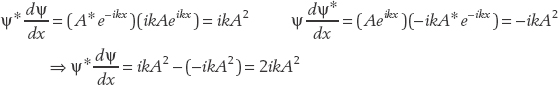
1. Divide up the problem into different regions, with each region representing a different potential. Figure 3-8 is a plot showing a piecewise constant potential. Each time the potential changes, we define a new region. In Fig. 3-8 there are four regions.

FIGURE 3-8
2. Solve the Schrödinger equation in each region. If the particles are in an unbound region (E > V), the wavefunction will be in the form of free particle states:
Remember that the term Ae ikx represents particles moving from the left to the right (from negative x to positive x), while Be-ikx represents particles moving from right to left. In a region where the particles encounter a barrier (E < V), the wavefunction will be in the form
3. The first goal in a scattering problem is to determine the constants A, B, and C. This is done by using two facts:
a. The wavefunction is continuous at a boundary. If we label the boundary point by a, then
b. The first derivative of the wavefunction is continuous at a boundary. Therefore we can use
We will see below that there is one exception to rule b: the derivative of the wavefunction is not continuous across a boundary when that boundary is a Dirac delta function.
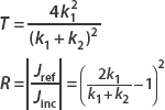
4. An important goal in scattering problems is to solve for the reflection and transmission coefficients. This final piece of the problem tells you whether particles make it past a barrier or not.
DEFINITION: Transmission and Reflection Coefficients
A scattering problem at a potential barrier will have an incident particle beam, reflected particle beam, and transmitted particle beam. The transmission coefficient T and reflection coefficient R are defined by
where the current density J is given by
To continue our summary of scattering:
5. When particles with E < V encounter a potential barrier represented by V, there will be penetration of the particles into the classically forbidden region. This is represented by a wavefunction that decays exponentially in that region. This is a quantum mechanical phenomenon called tunneling through the barrier. If particles are moving from left to right, the wavefunction is of the form
While particles penetrate into the region, there is 100% reflection. So we expect R = 1, T = 0.
6. The reflection and transmission coefficients give us the fraction of particles that are reflected or transmitted, so R + T = 1.
7. When the energy of particles is greater than the potential on both sides of a barrier (E > V), the wavefunction will be
on the left of the barrier while on the other side of the discontinuity, it will be
Here the subscripts i and j represent different sides of the barrier (regions 1 and 2, for example). The particular constraints of the problem may force us to set one or more of A, B, C, and D to zero. The constants k1 and k2 are found by solving the Schrödinger equation in each region:
where E is the energy of the incident particles and Vi is the potential in region i (and we are assuming that E > Vi). The constants k1and k2 are set to
As E increases, we find that k1 → k2 and R → 0, T → 1. On the other hand, if E is smaller and approaches V2, then R → 1 and T → 0.
A beam of particles coming from x = –∞ meets a potential barrier described by V (x) = V, where V is a positive constant, at x = 0. Consider the incident beam of particles to have energy 0 < E < V. Find the wavefunction for x < 0 and for x > 0, and describe the transmission and reflection coefficients for this potential.
A plot of the potential is shown in Fig. 3-9. The energy of the incoming particles is indicated qualitatively by the dashed line, while the solid line represents V(x) = V for x > 0.

FIGURE 3-9
To solve a problem like this, we divide the problem into two regions. We label x < 0 as region I. In this region, the potential is zero, and so the beam of particles is described by the free particle wavefunction. A particle coming from the left and moving to the right, which we label as the incident wavefunction, is described by
When the beam encounters a potential barrier, some particles will be reflected. So the total wavefunction in region I is given by a sum of incident this plus reflected wavefunctions. The reflected wavefunction, which moves to the left, is e–ikx. We write the total wavefunction in region I as
For x > 0, the Schrödinger equation becomes
Moving all terms to the left and dividing through by  , we obtain
Since 0 < E < V, the term
If we call this term β2, the equation becomes
There are two solutions to this familiar equation:
We reject the first solution because it blows up as x → ∞ and is physically unacceptable. Therefore in region II, we find that
So, to the left of the barrier, the wavefunction is oscillatory, while to the right it decays exponentially. We can represent this qualitatively by the plot in Fig. 3-10.

FIGURE 3-10
DEFINITION: Conditions That the Wavefunction Must Obey at a Discontinuity
The wavefunction must obey two conditions:
1. ψ must be continuous.
2. The first derivative dψ/dx must be continuous.
The boundary in this problem is at x = 0. To the left of the boundary, the wavefunction is
Setting x = 0, we get ψ(0) = A + B. For x > 0,
Matching up the wavefunction at x = 0 gives the condition
A + B = C
For x < 0, dψ/dx is
while for x > 0 we have
Letting x = 0 and setting both sides equal to each other, we obtain
Using A + B = C, we have
Solving allows us to write

Solving the schrödinger equation requires nothing special—just use basic techniques for solving partial differential equations:
• Consider each region separately, where you define your regions by what the potential V is over a given range.
• Apply initial conditions where necessary.
• Apply boundary conditions to match up your solutions.
Now, to find the transmission and reflection coefficients, we calculate the probability current density for each wavefunction. This is given by
For 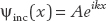 , we find
Therefore,
So we obtain
A similar procedure shows that
Now we calculate the current density for the transmitted current. The wavefunction for x > 0 is

The reflection coefficient is found to be

As expected, there is particle penetration into the barrier, but this tells us that no particles make it past the barrier—there is 100% reflection.
In this example we consider the same potential barrier, but this time we take E > V.
This time the energy of the incoming beam of particles is greater than that of the potential barrier. A schematic plot of this situation is shown in Fig. 3-11.
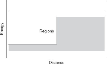
FIGURE 3-11
We call the region left of the barrier (x < 0) region I while region II is x > 0. To the left of the barrier in region I, the situation is exactly the same as it was in Example 3-2. So the wavefunctions are
This time, since E > V, the Schrödinger equation has the form
Now E > V, and so V − E < 0, and we have
where
represents the wavenumber in region II. The solution to the Schrödinger equation in region II is
However, the term  represents a beam of particles moving to the left toward –x and from the direction of x = +∞. The problem states that the incoming beam comes from the left; therefore there are no particles coming from the right in region II. Therefore D = 0 and we take the wavefunction to be
The procedure to determine the current densities in region I is exactly the same as it was in the last problem. Therefore,

In region II, this time the calculation of the current density is identical to that used for Jinc and Jref; however, we let k → ∞, giving
Continuity of the wavefunction at x = 0 leads to the same condition that was found in Example 3-2:

In region I, the derivative at x = 0 is also the same as it was in Example 3-2:
In region II, this time
And so the matching condition of the derivatives at x = 0 becomes
From A + B = C, we substitute B = C – A and obtain
or
This leads to
It can be verified that
Recall that in region I we have a free particle. So
In region II, we found that
Therefore, the ratio between the wavenumbers in the two regions is

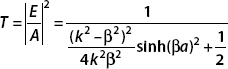
Incident particles of energy E coming from the direction of x = – ∞ are incident on a square potential barrier V, where E < V (see Fig. 3-12).

FIGURE 3-12
The potential is V for 0 < x < a and is 0 otherwise. Find the transmission coefficient.
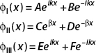
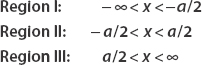
We divide this problem into three regions:

With the definitions
the wavefunctions for each of the three regions are
The incident particles are coming from x = –∞, so F = 0. Matching the wavefunctions at x = 0 gives
Matching x = a gives
Continuity of the first derivative at x = 0 gives
and at x = a
Combining the matching condition of the wavefunction and the first derivative at x = 0 yields
Doing the same at x = a gives
Combining these two results, we find

Recalling that
we will rewrite the ratio A/E. First we proceed as follows:
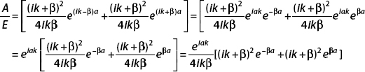
Now we expand the terms:
Putting this into the above result gives
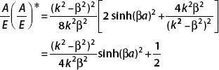
The transmission coefficient will be calculated using the modulus squared of this quantity. For a complex number z, we recall that |z|2 = zz*. The complex conjugate of this expression is
Now,
We make the following definition:

Putting these results together, we obtain

Now we use the hyperbolic trig identities:
The ratio then becomes
Finally, the transmission coefficient is
Parity
The parity operator P acts on a wavefunction in the following way:
Now consider the eigenvalue equation for P:
Application of P a second time in the first equation gives
We apply this to the eigenvalue equation:
Equating these two results, we have
Are the eigenvalues of parity? An even function for which ψ(–x) = (x) is seen to have the eigenvalue +1 and can be said to have even parity. An odd function for which −ψ (−x) = –ψ(x) corresponds to the eigenvalue –1 and is said to have odd parity. The even and odd parts of any wavefunction can be constructed using
When the potential is symmetric, so that V(x) = V(–x), the Hamiltonian H commutes with the parity operator. This means that if ψ(x) is an eigenfunction of H, so is Pψ(x).
Find the possible energies for the square well defined by

A qualitative plot of the potential is shown in Fig. 3-13.

FIGURE 3-13
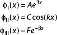
Following the procedure used in Example 3-4, we define three regions:
We again define
with the wavefunctions

The condition that ϕ → 0 as x → ± ∞ requires us to set B = 0 and E = 0.

In region II, notice that the well is centered about the origin. Therefore the solutions will be either even functions or odd functions. Even solutions are given in terms of cosine functions while odd solutions are given in terms of sine functions. We proceed with the even solutions. The odd solutions are similar.
The derivatives of these functions under those conditions are
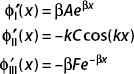
The wavefunction must match at the boundaries of the well. We can match it at x = a / 2, and so
The first derivative must also be continuous at this boundary, so
Dividing this equation by the first one gives
recalling that
The relation above is a transcendental equation that can be used to find the allowed energies. This can be done numerically or graphically. We rewrite the equation slightly:
The places where these curves intersect give the allowed energies. These eigenvalues are discrete; the number of them that are found depends on the parameter
If λ is large, there will be several allowed energies, while if λ is small, there might be two or even just one bound state energy. A plot of Fig. 3-14 shows an example.

FIGURE 3-14
The procedure for the odd solutions is similar, except you will arrive at a cosine function instead of the tangent.
Suppose that
where V > 0.
(a) Let E < 0 and find the bound state wavefunction and the energy.
(b) Let an incident beam of particles with E > 0 approach from the direction of x = –∞, and find the reflection and transmission coefficients.
(a) If we let  , the Schrödinger equation is
We consider two regions. Region I, for – ∞ < x < 0, has
We take functions of the form Aeβx because we are seeking a bound state. The requirement that ψ → 0 as x → –∞ for a bound state forces us to set B = 0. In region II,
The requirement that ψ → 0 as x → ∞ forces us to set C = 0. So the wavefunctions are
Even with a delta function potential, continuity of the wavefunction is required. Continuity of ψ at x = 0 tells us that
A = D
The derivative of the wavefunction is not continuous. We can find the discontinuity by integrating the term  . We can integrate about the delta function from ± ∈ where ∈ is a small parameter, and let ∈ → 0 to find out how the derivative behaves. Let’s recall the Schrödinger equation:
Examining the last term, we integrate over ±∈ and use the fact that ψ (0) = A:

Letting ∈ → 0, we see that this term vanishes. This leaves two terms that we need to calculate.

The first term is
x = +∈ corresponds to the wavefunction in region II.
Using
we have
and so
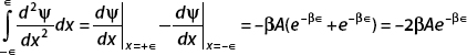
As ∈ → 0, this becomes
Integrating  , we use the sampling property of the delta function:
where we used  and the continuity of the wavefunction at x = 0 which required us to set D = A.
Using  , we find the energy to be
The wavefunction, which we found to be
can be written compactly as
Figure 3-15 is a plot of the wavefunction. Here A is found by normalization. In fact, we visited this wavefunction in Chap. 2. There we took

FIGURE 3-15
and found the normalization constant to be given by
In the present case, with  , we have
(b) For E > 0, the wavefunctions are, for particles incident from x → – ∞,
Continuity at x = 0 gives
The derivatives are
The first derivative is again discontinuous in this case. Proceeding as in part (a),
Letting ∈ → 0, we obtain
Since A + B = C, we can take ψ (0) to be either term. We will set ψ (0) = C. Then

gives us, in this case,
The transmission coefficient is found from C/A:

Using T + R = 1, the reflection coefficient is

Ehrenfest Theorem
Consider the time derivative of the expectation value of x (we assume that x does not depend directly on time):
Now we use 

Now  , so
, so
Now evaluating the time rate of change of  , we find that

These results together give us the Ehrenfest theorem, which states that the laws of classical mechanics embodied in Newton’s laws hold for the expectation values of the quantum operators x and p. This establishes a correspondence between classical and quantum dynamics.
Summary
In this chapter we learned about kinetic energy and momentum of the free particle, and energy degeneracy. Next we learned how to handle quantum states and simple 1-D scattering. Finally, Ehrenfest theorem connects classical and quantum mechanics through expectation values.
QUIZ
1. The Schrödinger equation for a free particle can be written as
A. 
B. 
C. 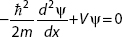
2. Degeneracy with respect to an energy eigenstate can be best described by saying that
A. Two or more different particle states have the same energy.
B. An energy eigenstate has at least two different energies.
C. Two or more particle states have zero momentum.
3. A dispersion relation is a functional relationship that
A. Relates energy and momentum
B. Relates frequency and wavenumber
C. Defines group velocity in terms of the particles state
4. The transmission coefficient is the magnitude of
A. ρ/J
B. Jtrans
C. Jtrans /Jinc
5. The transmission and reflection coefficients obey which of the following?
A. T + R = 1
B. T – R = 1
C. 
6. To solve the Schrödinger equation with different potentials over different regions of space
A. Average the potential and then solve the Schrödinger equation, using the averaged potential over all regions.
B. Solve the Schrödinger equation in each region independently and then match up boundary conditions.
C. Solve the free particle equation in all regions, and then add a solution obtained by taking the averaged potential over all regions.
D. Solve the Schrödinger equation in each region independently and then match up the initial conditions.
7. Ehrenfest theorem
A. Relates the time derivative of the average value of a quantum mechanical operator to the commutator of that operator with the Hamiltonian
B. Relates the time derivative of the value of a quantum mechanical operator to the commutator of that operator with the Hamiltonian
C. Relates the time derivative of the value of a quantum mechanical operator to the average value of the commutator of that operator with the Hamiltonian
D. Does as in part A, and it only applies to the free particle
8. The eigenvalues of the parity operator are
A. 0
B. ±
C. ±1
D. ±E where E is the energy of the particle
..................Content has been hidden....................
You can't read the all page of ebook, please click here login for view all page.