FEM for Frames
6.1 Introduction
A frame element is formulated to model a straight bar of an arbitrary cross-section, which can deform not only in the axial direction but also in the directions perpendicular to the axis of the bar. The bar here is capable of carrying both axial and transverse forces, as well as moments. Therefore, a frame element is seen to possess the properties and capabilities of both truss and beam elements. In fact, the frame structure can be found in many real world structures. The developments of FEM equations for bar and beam elements facilitate the development of FEM equations for frame structures in this chapter.
The frame element developed in this chapter is also known in many commercial software packages as the general beam element, or even simply the beam element. Commercial software packages usually offer both pure beam and frame elements, but frame structures are more often used in actual engineering applications. A three-dimensional spatial frame structure can practically take forces and moments of all directions. Hence, it can be considered to be the most general form of element with a one-dimensional geometry.
Frame elements are applicable for the analysis of skeletal type systems of both planar frames (two-dimensional frames) and space frames (three-dimensional frames). A typical three-dimensional frame structure is shown in Figure 6.1. Structural members in a frame structure are joined together by welding so that both forces and moments can be transmitted between members. In the following formulation, we assume that the frame element has a uniform cross-sectional area. If a structure of varying cross-section is to be modeled using the formulation in this chapter, then one approach is to divide the structure into smaller elements each with a different but constant cross-sectional area so as to simulate the varying cross-section. If the variation in cross-section is too severe, then the equations for a varying cross-sectional area can also be formulated easily using the same concepts and procedures given in this chapter. The basic concepts, procedures, and formulations can also be found in many existing textbooks (see, for example, Petyt, 1990; Rao, 1999).

6.2 FEM equations for planar frames
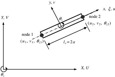
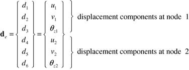
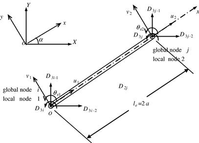
Consider a frame structure whereby the structure is divided into frame elements connected by nodes. Each element is of length le = 2a, and has two nodes at its two ends. The elements and nodes are numbered separately in a convenient manner. In a planar frame element, there are three degrees of freedom (DOFs) at one node in its local coordinate system, as shown in Figure 6.2. They are the axial deformation in the x direction, u; deflection in the y direction, v; and the rotation in the x–y plane and with respect to the z axis, θz. Therefore, each 2-node frame element has a total of six DOFs.
6.2.1 The idea of superposition
As mentioned, a frame element contains both the properties of the truss element and the beam element developed in the previous two chapters. Therefore, a simple way of formulating the element matrices is by superposition of the element matrices corresponding to the truss onto those of beam elements, without going through the detailed formulation process.
6.2.2 Equations in the local coordinate system
Considering the frame element shown in Figure 6.2 with nodes labeled 1 and 2 at each end of the element, it can be seen that the local x axis is taken as the axial direction of the element with its origin at the middle of the element. Recall that the truss element has only one DOF at each node (axial deformation), and the beam element has two DOFs at each node (transverse deformation and rotation). Combining these will give the three DOFs of a frame element, and the element displacement vector for a frame element can thus be written as
 (6.1)
(6.1)
To include the contribution of the stiffness matrix for the truss element, Eq. (4.15) is first extended to a 6 × 6 matrix corresponding to the order of the DOFs of the truss element in the element displacement vector in Eq. (6.1):
 (6.2)
(6.2)
Next, the stiffness matrix for the beam element, Eq. (5.23), is also extended to a 6 × 6 matrix corresponding to the order of the DOFs of the beam element in Eq. (6.1):
 (6.3)
(6.3)
The two matrices in Eqs. (6.2) and (6.3) are now superposed together to obtain the stiffness matrix for the frame element:
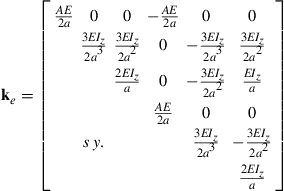 (6.4)
(6.4)
The element mass matrix of the frame element can also be obtained in the same way as the stiffness matrix. The element mass matrices for the truss element and the beam element, Eqs. (4.16) and (5.25), respectively, are extended into 6 × 6 matrices and added together to give the element mass matrix for the frame element:
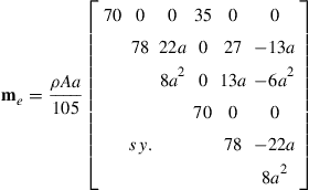 (6.5)
(6.5)
The same simple procedure can be applied to the force vector as well. The element force vectors for the truss and beam elements, Eqs. (4.17) and (5.25), respectively, are extended into 6 × 1 vectors corresponding to their respective DOFs and added together. If the element is loaded by external distributed forces fx and fy along the x axis; concentrated forces Fsx1, Fsx2, Fsy1, and Fsy2; and concentrated moments Ms1 and Ms2, respectively, at nodes 1 and 2, the total nodal force vector becomes
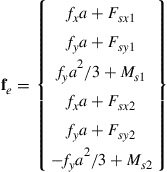 (6.6)
(6.6)
The final FEM equation for the frame element will thus have the form of Eq. (3.89) wherein the element matrices are given by Eqs. (6.4)–(6.6).
6.2.3 Equations in the global coordinate system
The matrices formulated in the previous section are in the local coordinate system of a frame element in a specific orientation. A full frame structure usually comprises numerous frame elements of different orientations joined together. As such, their local coordinate system would vary from one element to another. To assemble the element matrices together, all the matrices must first be expressed in a common coordinate system, which is the global coordinate system. The coordinate transformation process is the same as that discussed in Chapter 4 for truss structures.
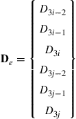
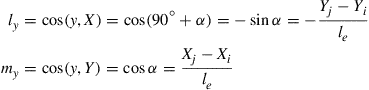
Assume that local nodes 1 and 2 correspond to the global nodes i and j, respectively. The displacement at a local node should have two translational components in the x and y directions and one rotational deformation. They are numbered sequentially by u, v, and θz at each of the two nodes, as shown in Figure 6.3. The displacement at a global node should also have two translational components in the X and Y directions and one rotational deformation. They are numbered sequentially by D3i−2, D3i−1, and D3i for the ith node, as shown in Figure 6.3. The same notation convention also applies to node j. The coordinate transformation gives the relationship between the displacement vector de based on the local coordinate system and the displacement vector De for the same element based on the global coordinate system:
![]() (6.7)
(6.7)
 (6.8)
(6.8)
and T is the transformation matrix for the frame element given by
 (6.9)
(6.9)
in which
 (6.10)
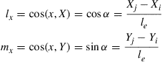
where α is the angle between the local x axis and the global X axis, as shown in Figure 6.3, and
 (6.11)
Note that the coordinate transformation in the X–Y plane does not affect the rotational DOF, as its direction is in the z direction (normal to the x–y plane), which still remains the same as the Z direction in the global coordinate system. The length of the element, le, can be calculated by
![]() (6.12)
(6.12)
Equation (6.7) can be easily verified, as it simply says that at node i, u1 equals the summation of all the projections of D3i−2 and D3i−1 onto the local x axis, and v1 equals the summation of all the projections of D3i−2 and D3i−1 onto the local y axis. The same can be said at node j. The matrix T for a frame element transforms a 6 × 6 matrix into another 6 × 6 matrix. Using the transformation matrix, T, the matrices for the frame element in the global coordinate system become
![]() (6.13)
(6.13)
![]() (6.14)
(6.14)
![]() (6.15)
(6.15)
Note that there is no change in dimension between the matrices and vectors in the local and global coordinate systems. Note also that the symmetry of the stiffness and mass matrices are all preserved in the coordinate transformation.
6.3 FEM equations for space frames
6.3.1 Equations in the local coordinate system
The approach used to develop the two-dimensional planar, frame elements can be used to develop the three-dimensional frame elements as well. The only difference is that there are more DOFs at a node in a 3D frame element than there are in a 2D frame element. There are altogether six DOFs at a node in a 3D frame element: three translational displacements in the x, y, and z directions, and three rotations with respect to the x, y, and z axes. Therefore, for an element with two nodes, there are altogether twelve DOFs, as shown in Figure 6.4.

The element displacement vector for a frame element in space can be written as
 (6.16)
The element matrices can be obtained by a similar process of obtaining the matrices of the truss element in space and that of beam elements, and adding them together. Because of the huge matrices involved, the details will not be shown in this book, but the stiffness matrix is listed here as follows, and can be easily confirmed simply by inspection:
 (6.17)
where Iy and Iz are the second moment of area (or moment of inertia) of the cross-section of the beam with respect to the y and z axes, respectively. Note that the fourth DOF is related to the torsional deformation. The formulation of a torsional bar element is very similar to that of a truss element. The only difference is that the axial deformation is replaced by the torsional angular deformation, and axial force is replaced by torque. Therefore, in the resultant stiffness matrix, the element tensile stiffness AE/le is replaced by the element torsional stiffness GJ/le, where G is the shear module and J is the polar moment of inertia of the cross-section of the bar.
The mass matrix can also be expressed by inspection as follows:
 (6.18)
where
![]() (6.19)
(6.19)
in which Ix is the second moment of area (or moment of inertia) of the cross-section of the beam with respect to the x axis.
6.3.2 Equations in the global coordinate system
Having set up the element matrices in the local coordinate system, the next thing to do is to transform the element matrices into the global coordinate system to account for the differences in orientation of all the local coordinate systems (now in 3D) that are attached on individual frame members.
Assume that the local nodes 1 and 2 of the element correspond to global nodes i and j, respectively. The displacement at a local node should have three translational components in the x, y, and z directions, and three rotational components with respect to the x, y, and z axes. They are numbered sequentially by d1–d12 corresponding to the physical deformations as defined by Eq. (6.16). The displacement at a global node should also have three translational components in the X, Y, and Z directions, and three rotational components with respect to the X, Y, and Z axes. They are numbered sequentially by D6i−5, D6i−4, …, D6i for the ith node, as shown in Figure 6.5. The same sign convention applies to node j. The coordinate transformation gives the relationship between the displacement vector de based on the local coordinate system and the displacement vector De based on the global coordinate system:
![]() (6.20)
(6.20)
 (6.21)
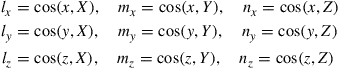
and T is the transformation matrix for the truss element given by
 (6.22)
in which
 (6.23)
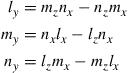
where lk, mk, and nk (k = x, y, z) are direction cosines defined by
 (6.24)
To define these direction cosines, the position and the three-dimensional orientation of the frame element have to be defined first. With nodes 1 and 2, the location of the element is fixed on the local coordinate frame, and the orientation of the element has also been fixed in the x direction. However, the local coordinate frame can still rotate about the axis of the beam. One more additional point in the local coordinate has to be defined. This point can be chosen anywhere in the local x–y plane, but not on the x axis. Therefore, node 3 is chosen, as shown in Figure 6.6.

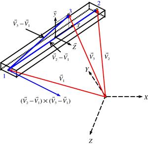
Figure 6.6 Vectors for defining the location and three-dimensional orientation of the frame element in space.
The position vectors ![]() ,
, ![]() , and
, and ![]() can be expressed as
can be expressed as
![]() (6.25)
(6.25)
![]() (6.26)
(6.26)
![]() (6.27)
(6.27)
where Xk, Yk, and Zk (k = 1, 2, 3) are the coordinates for node k, and ![]() and
and ![]() are unit vectors along the X, Y, and Z axes. We now define
are unit vectors along the X, Y, and Z axes. We now define
 (6.28)
Vectors ![]() and
and ![]() can thus be obtained using Eqs. (6.25)–(6.28) as follows:
can thus be obtained using Eqs. (6.25)–(6.28) as follows:
![]() (6.29)
(6.29)
![]() (6.30)
(6.30)
The length of the frame element can be obtained by
![]() (6.31)
(6.31)
The unit vector along the x axis can thus be expressed as
 (6.32)
Therefore, the direction cosines in the x direction are given as
 (6.33)
From Figure 6.6, it can be seen that the direction of the z axis can be defined by the cross product of vectors ![]() and
and ![]() . Hence, the unit vector along the z axis can be expressed as
. Hence, the unit vector along the z axis can be expressed as
 (6.34)
Substituting Eqs. (6.29) and (6.30) into the above equation,
![]() (6.35)
(6.35)
where
![]() (6.36)
(6.36)
Using Eq. (6.35), it is found that
 (6.37)
Since the y axis is perpendicular to both the x axis and the z axis, the unit vector along the y axis can be obtained by cross product,
![]() (6.38)
(6.38)
which gives
 (6.39)
in which lx, mx, nx, lz, mz, and nz have been obtained using Eqs. (6.33) and (6.37).
Using the transformation matrix, T, the matrices for space frame elements in the global coordinate system can be obtained, as before, as
![]() (6.40)
(6.40)
![]() (6.41)
(6.41)
![]() (6.42)
(6.42)
6.4 Remarks
In the formulation of the matrices for the frame element in this chapter, the superposition of the truss element and the beam element have been used. This technique assumes that the axial effects are not coupled with the bending effects in the element. What this means is simply that the axial forces applied on the element will not result in any bending deformation, and the bending forces will not result in any axial deformation. Frame elements can also be used for frame structures with curved members. In such cases, the coupling effects can exist even in the elemental level. Therefore, depending on the curvature of the member, the meshing of the structure can be very important. For example, if the curvature is very large, resulting in a significant coupling effect, a finer mesh is required to provide the necessary accuracy. In practical structures, it is very rare to have beam structures subjected to purely transverse loading. Most skeletal structures are either trusses or frames that carry both axial and transverse loads. It can now be seen that the beam element, developed in Chapter 5, as well as the truss element, developed in Chapter 4, are simply specific cases of the frame element. Therefore, in most commercial software packages, including ABAQUS, the frame element is just known generally as the beam element.
The beam element, formulated in Chapter 5, or general beam element, formulated in this chapter, is based on the so-called Euler–Bernoulli beam theory that is suitable for thin beams with a small thickness-to-span ratio (<1/20). For thick or deep beams of a large thickness-to-span ratio, corresponding beam theories should be used to develop thick beam elements. The procedure of developing thick beams is very similar to that of developing thick plates (discussed in Chapter 8) and most commercial software packages offer thick beam elements as well.
6.5 Case study: finite element analysis of a bicycle frame
In the design of many modern devices and pieces of equipment, the finite element method has become an indispensable tool for many of the successful products that we have come to use daily. In this case study, the analysis of a bicycle frame is carried out. Historically, intuition and trial-and-error in physical prototype testing have played important roles in coming out with the evolution of the diamond-shaped bicycle frame, as shown in Figure 6.7. However, using such a physical trial-and-error design procedure is costly and time consuming, and has its limitations, especially when new materials are introduced and when new applications or demands are placed on the structure. Hence, there is the need to use the finite element tool to help the designer come up with reliable properties in the design to meet the demands expected by consumers. Using the FEM to perform a virtual prototyping instead of a physical prototyping can save lots of cost, time, and effort. There can be numerous factors to consider when it comes to designing a bicycle frame. For example, factors like the weight of the frame, the maximum load the frame can carry, the impact toughness of the frame, and so on. In an FE analysis, one would require information on the material properties, the boundary conditions, and the loading conditions. The actual loading conditions on a bicycle can be extremely complex, especially when a rider is riding a bicycle and going through different terrain. In this case study we simply consider a loading condition of a horizontal impact applied to the bicycle, simulating the effect of a low speed, head-on collision into a wall or curb. This case is one of the physical tests that manufacturers have to comply with before a bicycle design is approved.

6.5.1 Modeling
The bicycle frame to be modeled is made of aluminum, whose properties are shown in Table 6.1. The bicycle frame is meshed by two-nodal “beam elements” in ABAQUS. Note that in ABAQUS, as well as in many other software packages, a general beam element in space is basically the same as the frame element developed in this chapter. The “beam element” in space offered by ABAQUS has the same DOFs as the frame element in this chapter, that is, three translational DOFs and three rotational DOFs.
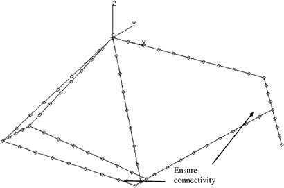
Altogether, 74 elements (71 nodes) are used in the skeletal model of the bicycle frame, as shown in Figure 6.8. Note that like all finite element meshes, connectivity at the nodes is very important. It is important to make sure that at the joints, there is connectivity between the elements. No node should be left unattached to another element unless the node happens to be at the end of a structure.
To model the horizontal impact, the two nodes at the rear dropouts are constrained from any displacements and a horizontal force of 1000 N is applied to the front dropout. The forces and constraints are shown in Figure 6.9.

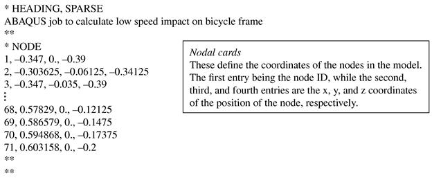
6.5.2 ABAQUS input file
The ABAQUS input file for the above described finite element model is shown below. The text boxes to the right of the input file are not part of the file, but explain what the sections of the file mean.

The above input file actually looks similar to that in Chapter 5. In fact, most ABAQUS input files have similar formats, only the information provided may be different depending on the problem required to solve.
6.5.3 Solution processes
The nodal and element cards provide information on the dimensions, position of nodes, and the connectivity of the elements. As discussed, these parameters play important roles in the formation of the element stiffness and mass matrices. Note that in the element cards, the element type specified is B33 which represents a general “beam element” in space with two nodes following the Euler–Bernoulli beam theory for its transverse displacement field. In ABAQUS, this would be exactly the same as the frame element developed in this chapter, since the DOFs also include the axial displacement component. ABAQUS, like most other software, does not have a pure beam element consisting of only the transverse displacement field. This is because not many real structures are a true beam structure without the axial displacement components. Hence, readers should not be confused by the use of beam elements in this case.
Next, the material properties and the cross-sectional geometry and dimensions are provided in the material cards and properties cards, respectively. As can be seen in Eqs. (6.4) and (6.5), the material properties, as well as the moment of area, are required to compute the stiffness and mass matrices. It is interesting to note that most of the information provided goes into forming the finite element matrices. In fact, that is the basic idea when it comes to applying the FEM: To form the finite element matrix equation and solve the equation to obtain the required field variables.
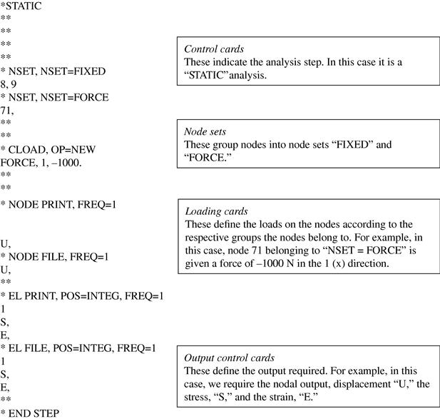
The next card would be the definition of the boundary conditions. In this case, the rear dropouts that are represented by nodes 8 and 9 and grouped as a node set, “FIXED,” are constrained in all DOFs. Recall that in this case, since each node has six DOFs, we can actually reduce the size of the matrix here by eliminating 12 rows and columns each, just as we have done in worked examples in Chapters 4 and 5. For the loads, it is given as a concentrated force of −1000 N at node 71 in the X direction. This would be reflected in the force vector, Eq. (6.42).
The control cards control the type of analysis to be performed, which in this case is a static analysis. In static analyses, the static equation KD = F is solved for D, which is a vector of the displacements and rotations of the nodes in the model. The method used is usually efficient algorithms that solve the linear system of equations via the Gauss elimination method, which is mentioned in Section 3.5.
The last part of the input file would consist of the output control cards, which specify the type of output requested. In this case, the nodal displacement and rotation components (U) and the elemental stress (S) and strain (E) components are specified. With the input file written, one can then invoke ABAQUS to execute the analysis.
6.5.4 Results and discussion
Using the above input file, the finite element equation is solved and a deformation plot showing how the frame actually deforms under the specified loading is shown in Figure 6.10. The magnitude of the deformation is actually magnified 20 times as the true deformation is too small for viewing purposes. Such deformation plots, or the results containing the displacements of the nodes, are useful to a designer since he or she will then be able to visualize the way in which the frame will deform under specific conditions. Furthermore, knowing the magnitude of deformation also helps to gauge aspects of the frame in the design, as consumers would not want a bicycle which could not be ridden once one accidentally hits a wall or curb at low speed.

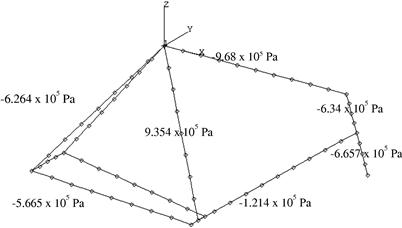
The other more important result that could be obtained from this case study would be the stresses that are incurred with this particular loading condition. Figure 6.11 shows the average axial stresses along the centroid of the aluminum beam members. It should be noted that it is possible to obtain stresses on different sections of the cross-section, for example, the upper or lower surface along the circumference of a circular cross-section. These stresses are useful for testing whether the bicycle frame will fail under the applied loads. If these stresses are smaller than the yield stress or the design stress of the material, then it can be safely concluded that there is a high chance that the material will not fail or undergo plastic deformation. It is important that the deformations remain elastic, that is, it will return to the original shape upon removal of the applied load.
Hence, it can be seen how the FEM can aid the design engineer when it comes to designing a product. It would be disastrous if a new design of an engineering system was mass-produced without going through any sort of analysis to check its reliability.
6.6 Review questions
1. Explain why the superposition technique can be used to formulate the frame elements simply by using the formulations of the truss and beam elements. Under what conditions will this superposition technique fail?
2. In the transformation from the local to the global coordinate system in a planar truss, does the rotational degree of freedom undergo any transformation? Why?
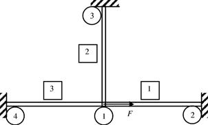
3. Work out the displacements of the planar frame structure shown in Figure 6.12. All the members are of the same material (E = 69.0 GPa, ν = 0.33) and with circular cross-sections. The areas of the cross-sections are 0.01 m2. Compare the results with those obtained for the Review Question 8 in Chapter 4.
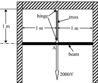
4. Figure 6.13 shows a supporting system consisting of a beam and a truss member, which carries a vertical load of 2000 N at point A that is at the middle span of the beam. Both the truss and beam members are of uniform cross-section and made of the same material with the Young’s modulus E = 200.0 GPa. The cross-section of the beam is circular, and the area of the cross-section is 0.01 m2. The area of the cross-section of the truss member is 0.0002 m2. Using the finite element method:
a. Calculate the nodal displacement at point A.
b. Calculate the reaction forces at the supports for the beam and truss member.
c. Calculate the internal forces in the truss member.
5. Figure 6.14 shows a supporting system consisting of one beam and two truss members, which carries a vertical uniformly distributed load of 2000 N/m on the top surface of the beam. The beam is clamped at the two ends into the rigid walls. Both the truss and beam members are of uniform cross-section and made of the same material with the Young’s modulus E = 200.0 GPa. The cross-section of the beam is circular, and the area of the cross-section is 0.01 m2. The area of the cross-section of the truss member is 0.0002 m2. Using the finite element method:
a. Calculate the nodal displacement at the middle span of the beam.
b. Calculate the reaction forces at the supports for the beam and truss member.
c. Calculate the internal forces in the truss member.

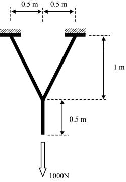
6. Figure 6.15 shows a simple frame consisting of three identical members: two horizontal and one vertical. These three members are joined firmly together at node 1. All the members are of length L = 2a, cross-sectional area A, Young’s modulus E and second moment of area I. A force F is applied horizontally at node 1. Using TWO frame elements, calculate the displacements and rotation at node 1, if any, in terms of F, L (or a), A, E, and I.
References
1. Petyt M. Introduction to Finite Element Vibration Analysis. Cambridge: Cambridge University Press; 1990.
2. Rao SS. The Finite Element in Engineering. third ed. Butterworth-Heinemann 1999.