FEM for Plates and Shells
8.1 Introduction
In this chapter, finite element (FE) equations for plates and shells are developed. The procedure is to first develop FE matrices for plate elements, and the FE matrices for shell elements are then obtained by superposing the matrices for plate elements and those for 2D solid plane stress elements developed in Chapter 7 (akin to superposing the truss and beam elements for the 1D frame elements). Unlike the 2D solid elements in the previous chapter, plate and shell elements are computationally more tedious as they involve more degrees of freedom (DOFs). The constitutive equations may seem daunting to one who may not have a strong background in the mechanics theory of plates and shells, and the integration may be quite involved if it is to be carried out analytically. However, the basic concepts of formulating the FE equation always remain the same. Readers are advised to pay more attention to the finite element concepts and the procedures outlined in developing plate and shell elements. After all, the computer can handle many of the tedious calculations/integrations that are required in the process of forming the elements. The basic concepts, procedures, and formulations can also be found in many existing textbooks (see, Petyt, 1990; Rao, 1999; Zienkiewicz and Taylor, 2000).
8.2 Plate elements
As discussed in Chapter 2, a plate structure is geometrically similar to the structure of the 2D plane stress problem, but it usually carries only transverse loads that lead to bending deformation in the plate. For example, consider the horizontal boards on a bookshelf that support the books. Those boards can be approximated as a plate structure, and the transverse loads are of course the weight of the books. Higher floors of a building are a typical plate structure that carries most of us every day, as are the wings of aircraft, which usually carry loads like the engines, as shown in Figure 2.13. The plate structure can be schematically represented by its middle plane laying on the x–y plane, as shown in Figure 8.1. The deformation caused by the transverse loading on a plate is represented by the deflection and rotation of the normals of the middle plane of the plate, and they will be independent of z and a function of only x and y. The element to be developed to model such plate structures is aptly known as the plate element. The formulation of a plate element is very much the same as for the 2D solid element, except for the process for deriving the strain matrix in which the theory of plates is used.

Plate elements are normally used to analyze the bending deformation of plate structures and the resulting forces such as shear forces and moments. In this respect, it is similar to the beam element developed in Chapter 5, except that the plate element is two dimensional whereas the beam element is one dimensional. Like the 2D solid element, a plate element can also be triangular, rectangular or quadrilateral in shape. In this book, we cover the development of the rectangular element only, as it is so widely used. Matrices for the triangular element can also be easily developed using similar procedures, and those for the quadrilateral element can be developed using the idea of an isoparametric element discussed for 2D solid elements. In fact, the development of a quadrilateral element is very much the same as the rectangular element, except for an additional procedure of coordinate mapping, as shown for the case of 2D solid elements.
There are a number of theories that govern the deformation of plates. In this chapter, rectangular elements based on the Mindlin plate theory that works for thick plates will be developed. Most books go into great detail to first cover plate elements based on the thin plate theory. However, most finite element packages do not use plate elements based on thin plate theory. In fact, most analysis packages like ABAQUS do not even offer the choice of plate elements. Instead, one has to use the more general shell elements, also discussed in this chapter. Furthermore, using the thin plate theory to develop the finite element equations has a problem, in that the elements developed are usually incompatible or “non-conforming.” This means that some components of the rotational displacements may not be continuous on the edges between elements. This is because the rotation depends only upon the deflection w in the thin plate theory, and hence the assumed function for w has to be used to calculate the rotation. Many texts go into even greater detail to explain the concept, and to prove the conformability of many kinds of thin plate elements. In our opinion, there is really no need, for most practical purposes, to understand such a concept and proof for readers who are interested in using the FEM to solve real-life problems. In addition, many structures may not be considered as a “thin plate,” or rather their transverse shear strains cannot be ignored. Therefore, the Reissner–Mindlin plate theory is more suitable in general, and the elements developed based on the Reissner–Mindlin plate theory are more practical and useful. This book will only discuss the elements developed based on the Reissner–Mindlin plate theory.
There are a number of higher order plate theories that can be used for the development of finite elements. Since these higher order plate theories are extensions of the Reissner–Mindlin plate theory, there should not be any difficulty for readers who can formulate the Mindlin plate element to understand the formulation of higher order plate elements.
It is assumed that the element has a uniform thickness h. If the plate structure has a varying thickness, the structure can be divided into small elements, each of uniform thickness, to approximate the overall variation in thickness. However, the formulation of plate elements with a varying thickness can also be done, as the procedure is similar to that of a uniform element; this would be good homework practice for readers after reading this chapter.
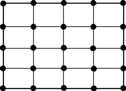
Consider now a plate that is represented by a two-dimensional domain in the x–y plane, as shown in Figure 8.1. The plate is divided in a proper manner into a number of rectangular elements, as shown in Figure 8.2. Each element will have four nodes and four straight edges. At a node, the DOFs include the deflection w, the rotation about x axis θx, and the rotation about y axis θy, making the total DOF of each node three. Hence, for a rectangular element with four nodes, the total DOF of the element would be twelve.
Following the Reissner–Mindlin plate theory (see Chapter 2), its shear deformation will force the cross-section of the plate to rotate in the way shown in Figure 8.3. Any straight fiber that is perpendicular to the middle plane of the plate before the deformation rotates, but remains straight after the deformation. The two displacement components that are parallel to the middle surface can then be expressed mathematically as
![]() (8.1)
(8.1)
![]()
where θx and θy are, respectively, the rotations of the vertical fiber of the plate with respect to the x and y axes. The in-plane strains can then be given as
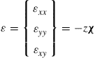 (8.2)
(8.2)
where χ is the curvature, given as
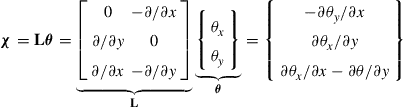 (8.3)
(8.3)
in which L is the differential operator defined in Chapter 2, and is re-written as
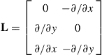 (8.4)
(8.4)
Since the vertical fiber of the plate (which is initially normal to the mid plane of the plate) rotates and no longer remains normal to the mid plane of the plate, there are off-plane shear strain components and these are given as
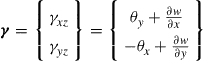 (8.5)
(8.5)
Note that Hamilton’s principle uses energy functions for derivation of the equation of motion. The potential (strain) energy expression for a thick plate element is
![]() (8.6)
(8.6)
The first term on the right-hand side of Eq. (8.6) relates to the in-plane stresses and strains, whereas the second term is for the transverse stresses and strains. τ is the average shear stresses relating to the shear strain in the form
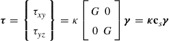 (8.7)
(8.7)
where G is the shear modulus, and κ is a shear correction factor to account for the non-uniformity of the shear stress across the thickness of the plate, while the transverse strains are uniform. This is because the Reissner–Mindlin plate theory assumes that the cross-section remains planar and hence the off-plane strains are uniform, but the actual off-plane shear stresses cannot be uniform: They have to be zero on the surfaces of the plate and maximum in the middle. The value of κ is usually taken to be π2/12 or 5/6.

Figure 8.3 Shear deformation in a plate. A straight fiber that is perpendicular to the middle plane of the plate before deformation rotates but remains straight after deformation.
Substituting Eqs. (8.2) and (8.7) into Eq. (8.6), the potential (strain) energy becomes
![]() (8.8)
(8.8)
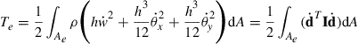
The kinetic energy of the thick plate is given by
![]() (8.9)
(8.9)
which is basically a summation of the contributions of three velocity components in the x, y, and z directions of all the particles in the entire domain of the plate. Substituting Eq. (8.1) into the above equation leads to
 (8.10)
where
 (8.11)
and
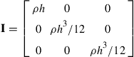 (8.12)
As we can see from Eq. (8.10), the terms related to in-plane displacements caused by the rotations are less important for thin plates, since it is proportional to the cubic of the plate thickness.
8.2.1 Shape functions
It can be seen from the above analysis of the constitutive equations that the rotations, θx and θy, are independent of the deflection w. Therefore, when it comes to interpolating the generalized displacements, the deflection and rotations can actually be interpolated separately using independent shape functions. Therefore, the procedure of field variable interpolation is the same as that for 2D solid problems, except that there are three instead of two DOFs, for a node.
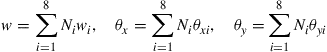
For four-node rectangular thick plate elements, the deflection and rotations can be summed as
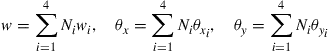 (8.13)
where the shape function Ni is the same as the four-node 2D solid element in Chapter 7, i.e.,
![]() (8.14)
(8.14)
The element constructed will be a conforming element, meaning that w, θx, and θy are continuous on the edges between elements. Rewriting Eq. (8.13) into a single matrix equation, we have
 (8.15)
where de is the (generalized) displacement vector for all the nodes in the element, arranged in the order
 (8.16)
and the shape function matrix is arranged in the order
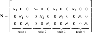 (8.17)
8.2.2 Element matrices
Once the shape function and nodal variables have been defined, element matrices can then be formulated following the standard procedure given in Chapter 7 for 2D solid elements. The only difference is that there are three DOFs at one node for plate elements.
To obtain the element mass matrix me and the element stiffness matrix ke, we have to use the energy functions given by Eqs. (8.8) and (8.9) and Hamilton’s principle. Substituting Eq. (8.15) into the kinetic energy function, Eq. (8.9) gives
![]() (8.18)
(8.18)
where the mass matrix me is given as
![]() (8.19)
(8.19)
The above integration can be carried out analytically, but it will be omitted here. Interested readers can refer to Petyt (1990) for details. In practice, we often perform the integration numerically using the Gauss integration scheme, discussed in Chapter 7.
To obtain the stiffness matrix ke, we substitute Eq. (8.15) into Eq. (8.6), from which we obtain
![]() (8.20)
(8.20)
The first term in the above equation represents the strain energy associated with the in-plane stress and strain. The strain matrix BI has the form of
![]() (8.21)
(8.21)
where
 (8.22)
Using the expression for the shape functions in Eq. (8.14), we obtain
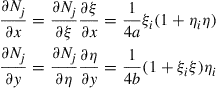 (8.23)
In deriving Eq. (8.23), the relationship given in Eq. (7.47) has been used.
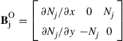
The second term in Eq. (8.20) relates to the strain energy associated with the off-plane shear stress and strain. The strain matrix BO has the form
![]() (8.24)
(8.24)
 (8.25)
The integration in the stiffness matrix ke, Eq. (8.20) can be evaluated analytically as well. Practically however, the Gauss integration scheme is used to evaluate the integrations numerically. Note that when the thickness of the plate is reduced, the element becomes over-stiff, a phenomenon that relates to so-called “shear locking.” The simplest and most practical means to alleviate this problem is to use 2 × 2 Gauss points for the integration of the first term, and use only one Gauss point for the second term in Eq. (8.20).
As for the force vector, we substitute the interpolation of the generalized displacements, given in Eq. (8.15), into the usual equation, as in Eq. (3.81), assuming that there is a distributed transverse force, fz, acting on the surface of the plate:
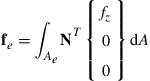 (8.26)
If the load is uniformly distributed in the element, fz is constant, and the above equation becomes
![]() (8.27)
(8.27)
Equation (8.27) implies that the distributed force is divided evenly into four concentrated forces of one quarter of the total force.
8.2.3 Higher order elements
For an eight-node rectangular thick plate element, the deflection and rotations can be summed as
 (8.28)
where the shape function Ni is the same as the eight-node 2D solid element given by Eq. (7.113). The element constructed will be a conforming element, as w, θx, and θy are continuous on the edges between elements. The formulation procedure is the same as for the rectangular plate elements.
8.3 Shell elements
A shell structure carries loads in all directions, and therefore undergoes bending and twisting, as well as in-plane deformation. Some common examples would be the dome-like design of the roof of a building with a large volume of space; or a building with special architectural requirements such as a church or mosque; or structures with a special functional requirement such as cylindrical and hemispherical water tanks; or lightweight structures like the fuselage of an aircraft, as shown in Figure 8.4. Shell elements are suitable for modeling such structures.

8.3.1 The idea of superposition
The simplest yet most widely used shell element can be formulated easily by superposing the 2D solid element formulated in Chapter 7 onto the plate element formulated in the previous section. The 2D solid elements handle the membrane or in-plane effects, while the plate elements are used to handle bending or off-plane effects. The procedure for developing such an element is very similar to the simple method of superposition used to formulate the frame elements using the truss and beam elements, as discussed in Chapter 6. Of course, the shell element can also be formulated using the usual method of defining shape functions, substituting into the constitutive equations based on shell theory, and thus obtaining the element matrices. However, as you might have guessed, it is going to be very tedious. Bear in mind, however, that the basic concept of deriving the finite element equation still holds, even though in this book, we introduce the simple method based on assembly. The derivation for four-nodal, rectangular shell elements will be outlined using the above-mentioned approach.
Since the plate structure can be treated as a special case of the shell structure, the shell element developed in this section is applicable for modeling plate structures. In fact, it is common practice to use a shell element offered in a commercial FE package to analyze plate structures.
8.3.2 Elements in the local coordinate system
Shell structures are usually curved. In our FEM formulation a shell-like structure is divided into shell elements that are flat. The curvature of the shell structure is then approximated by changing the orientation of the shell elements in space. Therefore, if the curvature of the shell is very large, a fine mesh of elements has to be used. Even though this assumption may sound like a crude approximation, it is very practical and widely used in engineering practice. There are alternatives of more accurately formulated shell elements, but they are used only in academic research and seldom implemented in any commercially available software packages. Therefore, we focus on the formulation of only flat shell elements in this book.
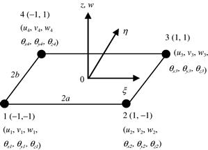
Similar to the frame structure, there are six DOFs at a node for a shell element: Three translational displacements in the x, y, and z directions, and three rotational deformations with respect to the x, y, and z axes. Figure 8.5 shows the middle plane of a rectangular shell element and the DOFs at the nodes. The generalized displacement vector for the element can be written as
 (8.29)
where di (i = 1, 2, 3, 4) are the displacement vector at node i:
 (8.30)
The stiffness matrix for a 2D solid, rectangular element is used to account for the membrane effects of the element, which corresponds to DOFs of u and v. The membrane stiffness matrix can thus be expressed in the following form using sub-matrices according to the nodes:
 (8.31)
where the superscript m stands for the membrane matrix. Each sub-matrix will have a dimension of 2 × 2, since it corresponds to the two DOFs u and v at each node. Note again that the matrix above is actually the same as the stiffness matrix of the 2D rectangular, solid element, except it is written in terms of sub-matrices according to the nodes.
The stiffness matrix for a rectangular plate element is used for the bending effects, corresponding to DOFs of w and θx, θy. The bending stiffness matrix can thus be expressed in the following form using sub-matrices according to the nodes:
 (8.32)
where the superscript b stands for the bending stiffness. Each bending sub-matrix has a dimension of 3 × 3.
The stiffness matrix for the shell element in the local coordinate system is then formulated by combining Eqs. (8.31) and (8.32):
 (8.33)
The stiffness matrix for a rectangular shell matrix has a dimension of 24 × 24. Note that in Eq. (8.33), the components related to the DOF θz are zeros. This is because there is no θz in the local coordinate system. If these zero terms are removed, the stiffness matrix would have a reduced dimension of 20 × 20. However, using the extended 24 × 24 stiffness matrix will make it more convenient for transforming the matrix from the local coordinate system into the global coordinate system.
Similarly, the mass matrix for a rectangular element can be obtained in the same way as for the stiffness matrix. The mass matrix for the 2D solid element is used for the membrane effects, corresponding to DOFs of u and v. The membrane mass matrix can be expressed in the following form using sub-matrices according to the nodes:
 (8.34)
where the superscript m stands for the membrane matrix. Each membrane sub-matrix has a dimension of 2 × 2.
The mass matrix for a rectangular plate element is used for the bending effects, corresponding to DOFs of w and θx, θy. The bending mass matrix can also be expressed in the following form using sub-matrices according to the nodes:
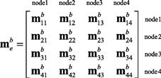 (8.35)
where the superscript b stands for the bending matrix. Each bending sub-matrix has a dimension of 3 × 3. The mass matrix for the shell element in the local coordinate system is then formulated by combining Eqs. (8.34) and (8.35):
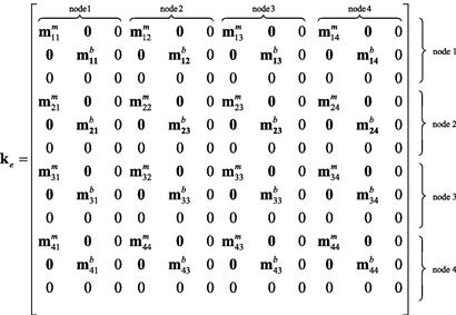 (8.36)
Similarly, it is noted that the terms corresponding to the DOF θz are zero for the same reasons as explained for the stiffness matrix.
8.3.3 Elements in the global coordinate system
The matrices for shell elements in the global coordinate system can be obtained by performing the transformations
![]() (8.37)
(8.37)
![]() (8.38)
(8.38)
![]() (8.39)
(8.39)
where T is the transformation matrix, given by
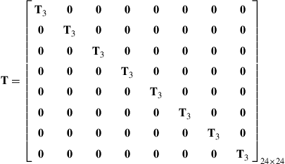 (8.40)
in which
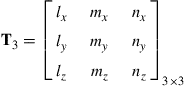 (8.41)
where lk, mk and nk (k = x, y, z) are direction cosines, which can be obtained in exactly the same way as described in Section 6.3.2. The difference is that there is no need to define the additional point 3, as there are already four nodes for the shell element. The local coordinates x, y, z can be conveniently defined under the global coordinate system using the four nodes of the shell element.
The global matrices obtained will not have zero columns and rows if the elements joined at a node are not in the same plane. If all the elements joined at a node are in the same plane, then the global matrices will be singular. This kind of case is encountered when using shell elements to model a flat plate. In such situations, special techniques, such as a “stabilizing matrix,” have to be used to solve the global system equations.
8.4 Remarks
The direct superposition of the matrices for 2D solid elements and plate elements are performed by assuming that the membrane effects are not coupled with the bending effects at the individual element level. This implies that the membrane forces will not result in any bending deformation, and bending forces will not cause any in-plane displacement in the element. For a shell structure in 3D space, the membrane and bending effects are actually coupled globally, meaning that the membrane force at an element may result in bending deformations in the other elements, and the bending forces in an element may create in-plane displacements in other elements. The coupling effects are more significant for shell structures with a strong curvature. Therefore, for those structures, a finer element mesh should be used. Using the shell elements developed in this chapter implies that the curved shell structure has to be meshed by piecewise flat elements. This simplification in geometry needs to be taken into account when evaluating the results obtained.
8.5 Case study: Natural frequencies of the micro-motor
In this case study, we examine the natural frequencies and mode shapes of the micro-motor described in Section 7.10. Natural frequencies are properties of a system, and it is important to study the natural frequencies and corresponding mode shapes of a system, because if a forcing frequency is applied to the system near to or at the natural frequency, resonance will occur. That is, there will be very large amplitude vibration that might be disastrous in some situations. In this case study, the flexural vibration modes of the rotor of the micro-motor will be analyzed.
8.5.1 Modeling
The geometry of the micro-motor’s rotor will be the same as that of Figure 7.22, and the elastic properties will remain unchanged using the properties in Table 7.2. To show the mode shapes more clearly, we model the rotor as a whole rather than as a symmetrical quarter model. However, using a quarter model is still possible, but one has to take note of symmetrical and anti-symmetrical modes (to be discussed in more detail in Chapter 11). Figure 8.6 shows the finite element model of the micro-motor containing 480 nodes and 384 elements. To study the flexural vibration modes, plate elements discussed in this chapter are used. However, as mentioned earlier in this chapter, most commercial finite element packages, including ABAQUS, do not allow the use of pure plate elements. Therefore, shell elements will be utilized here for meshing up the model of the micro-motor. 2D, four-nodal shell elements (S4) are used. Recall that each shell element has three translational DOFs and three rotational DOFs, and it is actually a superposition of a plate element with a 2D solid element. Hence, to obtain just the flexural modes, we would need to constrain the DOFs corresponding to the x translational displacement and the y translational displacement, as well as the rotation about the z axis. This would leave each node of a shell element with the three DOFs of a plate element. As before, the nodes along the edge of the center hole will be constrained to be fixed. Since we are interested in the natural frequencies, there will be no external forces on the rotor.

8.5.2 ABAQUS input file
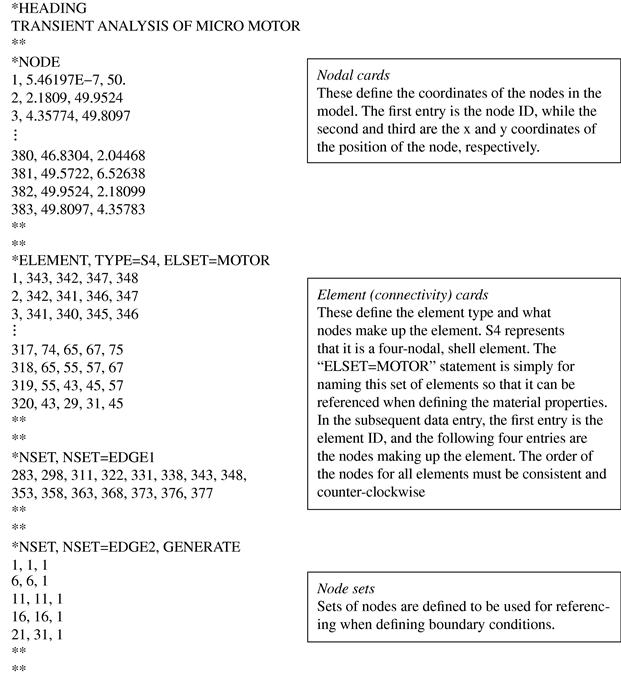
The ABAQUS input file for the problem described is shown below. Note that some parts are not shown due to limitations of space available in this text.


8.5.3 Solution process
Looking at the mesh in Figure 8.6, one can see that quadrilateral shell elements are used. Therefore, the equations for a linear, quadrilateral shell element must be formulated by ABAQUS. As before, the formulation of the element matrices would require information from the nodal cards and the element connectivity cards. The element type used here is S4, representing four-nodal shell elements. There are other types of shell elements available in the ABAQUS element library.
After the nodal and element cards, next to be considered would be the property and material cards. The properties for the shell element used here must be defined, which in this case includes the material used and the thickness of the shell elements. The material cards are similar to those of the case study in Chapter 7, except that here the density of the material must be included, since we are not carrying out a static analysis, as in Chapter 7.
The boundary (BC) cards then define the boundary conditions on the model. In this problem, we would like to obtain only the flexural vibration modes of the motor, hence the components of displacements in the plane of the motor are not actually required. As mentioned, this is very much the characteristic of the plate elements. Therefore, DOFs 1, 2, and 6 corresponding to the x and y displacements, and rotation about the z axis, are constrained. The other boundary condition would be the constraining of the displacements of the nodes at the center of the motor.
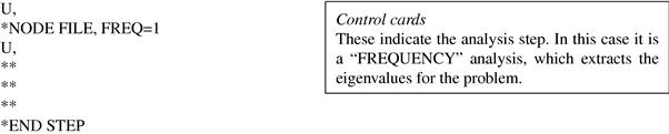
Without the need to define any external loadings, the control cards then define the type of analysis ABAQUS would carry out. ABAQUS uses the sub-space iteration scheme by default to evaluate the eigenvalues of the equation of motion. This method is a very effective method of determining a number of lowest eigenvalues and corresponding eigenvectors for a very large system of several thousand DOFs. The procedure is outlined in the case study in Chapter 5. Finally, the output control cards define the necessary output required by the analyst.
8.5.4 Results and discussion
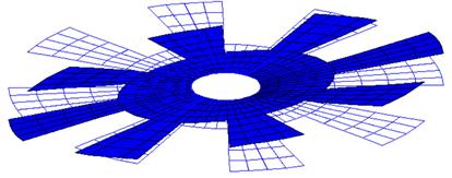
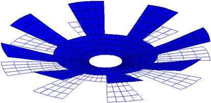
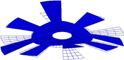
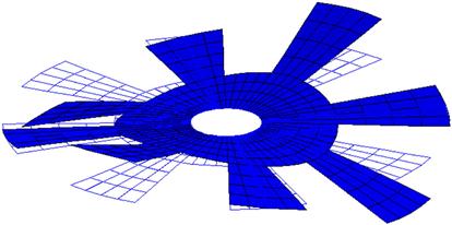
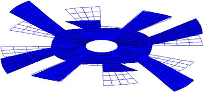
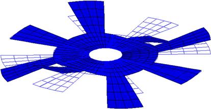
Using the input file above, an eigenvalue extraction is carried out in ABAQUS. The output is extracted from the ABAQUS results file showing the first eight natural frequencies and these are tabulated in Table 8.1. The table also shows results obtained from using triangular elements as well as a finer mesh of quadrilateral elements. It is interesting to note that for certain modes, the eigenvalues and hence the frequencies are repetitive with the previous one. This is due to the symmetry of the circular rotor structure. For example, modes 1 and 2 have the same frequency, and looking at their corresponding mode shapes in Figures 8.7 and 8.8, respectively, one would notice that they are actually of the same shape but bending at a plane 90° from each other. As such, many consider this as one single mode. Therefore, though eight eigenmodes are extracted, it is effectively equivalent to only five eigenmodes. However, to be consistent with the result file from ABAQUS, all the modes extracted will be shown here. Figures 8.9–8.14 show the other mode shapes from this analysis. Remember that, since the in-plane displacements are already constrained, these modes are only the flexural modes of the rotor.
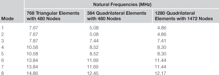


Comparing the natural frequencies obtained using 768 triangular elements with those obtained using the quadrilateral elements, one can see that the frequencies are generally higher using the triangular elements. Note that for the same number of nodes, using the quadrilateral elements requires half the number of elements. The results obtained using 384 quadrilateral elements do not differ much from those that use 1280 elements. This again shows that the triangular elements are less accurate than the quadrilateral elements. Note that the mode shapes obtained in the three analyses are the same. It is interesting to also note that the natural frequencies are higher (stiffer) when less elements are used, which shows the over-stiffening effect of the FEM. Using more elements relaxes the constrains from the shape functions more and hence the structure becomes softer.
8.6 Case study: Transient analysis of a micro-motor
While analyzing the micro-motor, another case study is included here to illustrate an example of a transient analysis using ABAQUS. The same micro-motor shown in Chapter 7 will be analyzed here.
The rotor of the micro-motor rotates due to the electrostatic force between the rotor and the stator poles of the motor. Let’s assume a hypothetical case where there is a misalignment between the rotor and the stator poles in the motor. As such, there might be other force components acting on the rotor. The actual analysis of such a problem can be very complex, so in this case study we simply analyze a very simple case of the problem with loading conditions as shown in Figure 8.15. It can be seen that symmetrical conditions are used, resulting in a quarter model. The transient response of the transverse displacement components of the various parts of the rotor is to be calculated here.

8.6.1 Modeling
Since we are analyzing the same structure as that in Chapter 7, the meshing aspects of the geometry will not be discussed again. It should be noted that an optimum number of elements (nodes) should be used for every finite element analysis. The same treatment of using the shell elements and constraining the necessary DOFs (1, 2, and 6) is carried out to simulate plate elements. The difference here is that there will be loadings in the form of a sinusoidal function with respect to time,
![]() (8.42)
(8.42)
applied as concentrated loadings at the positions shown in Figure 8.15.
8.6.2 Abaqus input file
The ABAQUS input file for the problem described is shown below. Note that some parts are not shown due to limitations of space available in this text.

8.6.3 Solution process
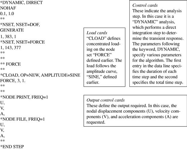
The significance of the information provided in the above input file is very similar to the previous case study. Therefore, this section will highlight the differences that are mainly used for the transient analysis.
The definition of the amplitude curve is important here as it enables the load (or boundary condition) to be defined as a function of time. In this case the load will follow the sinusoidal function defined in the amplitude curve block. The sinusoidal function is defined as a periodic function whereby the formula used is actually the Fourier series. The data lines in the amplitude curve block basically define the angular frequency and the other constants in the Fourier series.
The control card specifies that the analysis is a direct integration, transient analysis. In ABAQUS, Newmarks’s method (Section 3.7.2) together with the Hilber–Hughes–Taylor operator (1978) applied on the equilibrium equations, is used as the implicit solver for direct integration analysis. The time increment is specified to be 0.1 s, and the total time of the step is 1.0 s. As mentioned in Chapter 3, implicit methods involve the solving of the matrix equation at each individual increment in time, therefore the analysis can be rather computationally expensive. The algorithm used by ABAQUS is quite complex, involving the capabilities of having automatic deduction of the required time increments. Further details are, however, beyond the scope of this book.
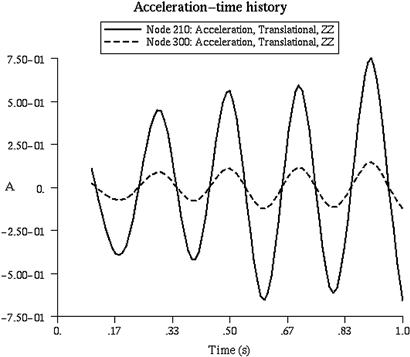
8.6.4 Results and discussion
Upon the analysis of the problem defined by the input file above, the displacement, velocity, and acceleration components throughout each individual time increment can be obtained until the final time step specified. Therefore, we have what is known as the displacement–time history, the velocity–time history and the acceleration–time history, as shown in Figures 8.16, 8.17, and 8.18, respectively. The plots show the displacement, velocity, and acceleration histories of nodes 210 and 300.


8.7 Review questions
1. If the plate were not homogenous but laminated, how would the finite element equation be different?
2. State the procedure to develop a triangular plate element.
3. Is it possible to develop plate elements using the classical plate theory (for thin plates)? What could be possible issues when doing so?
4. What could be a problem, if the plate elements developed based on the Mindlin plate theory (or other higher order theory) used for thin plates?
5. How should one develop a four-node quadrilateral element? How should one develop an eight-node element with curved edges?
6. How many Gauss points are required to obtain the exact results for Eqs. (8.19) and (8.20)?
7. Consider a uniform, isotropic square plate with a dimension of 1 m by 1 m. The plate is made of a material with Young’s modulus E = 70 GPa and Poisson ratio ν = 0.3. Using any FEM software package, compute the deflection, distribution of moments, shear forces, and a normal stress on the top surface of the plate. Using square elements with nodal density of 2 × 2, 4 × 4, 8 × 8, and 16 × 16 to perform the analysis, compare the FEM solution with the analytical solution (based on thin plate theory) for the deflection at the center of the plate. You are requested to perform the following studies:
a. The plate is of thickness 0.001 m and clamped on all edges (CCCC);
b. The plate is of thickness 0.01 m and clamped on all edges (CCCC);
c. The plate is of thickness 0.1 m and simply-supported on all edges (SSSS);
d. The plate is of thickness 0.001 m and simply-supported on all edges (SSSS);
e. The plate is of thickness 0.01 m and simply-supported on all edges (SSSS);
f. The plate is of thickness 0.1 m and simply-supported on all edges (SSSS);
g. The plate is of thickness 0.001 m, clamped on two opposite edges and simply-supported on the other two edges (CSCS);
h. The plate is of thickness 0.01 m, clamped on two opposite edges and simply-supported on the other two edges (CSCS);
i. The plate is of thickness 0.1 m, clamped on two opposite edges and simply-supported on the other two edges (CSCS).
References
1. Hilber HM, Hughes TJR, Taylor RL. Collocation, dissipation and “overshoot” for time integration schemes in structural dynamics. Earthquake Engineering and Structural Dynamics. 1978;6:99–117.
2. Petyt M. Introduction to Finite Element Vibration Analysis. Cambridge: Cambridge University Press; 1990.
3. Rao SS. The Finite Element in Engineering. third ed. Butterworth-Heinemann 1999.
4. Zienkiewicz OC, Taylor RL. The Finite Element Method. fifth ed. Butterworth-Heinemann 2000.