Chapter 15
Managing the DSP Software Development Effort
Chapter Outline
Challenges in DSP application development
Concept and specification phase
A specification process for DSP systems
Algorithm development and validation
DSP algorithm standards and guidelines
High level system design and performance engineering
System build, integration, and test
Design challenges for DSP systems
High level design tools for DSP
Host development tools for DSP development
Introduction
Software development using DSPs is subject to many of the same constraints and development challenges which other types of software development face. These include a shrinking time to market, tedious and repetitive algorithm integration cycles, time intensive debug cycles for real-time applications, and integration of multiple differentiated tasks running on a single DSP, as well as other real-time processing demands. Up to 80% of the development effort is involved in analysis, design, implementation, and integration of the software components of a DSP system.
Early DSP development relied on low level assembly language to implement the most efficient algorithms. This worked reasonably well for small systems. However, as DSP systems grow in size and complexity, assembly language implementation of these systems has become impractical. Too much effort and complexity is involved to develop large DSP systems within reasonable cost and schedule constraints. The migration has been towards higher level languages like C to provide the maintainability, portability, and productivity needed to meet cost and schedule constraints. Other real-time development tools are emerging to allow even faster development of complex DSP systems.
DSP development environments can be partitioned into host tooling and target content. Host tooling consists of tools to allow the developer to perform application development tasks such as program build, program debug, data visualization, and other analysis capabilities. Target content refers to the integration of software running on the DSP itself, including the real-time operating system (if needed), and the DSP algorithms that perform the various tasks and functions. There is a communication mechanism between the host and the target for data communication and testing.
DSP development consists of several phases as shown in Figure 15-1. During each phase there exists tooling to help the DSP developer quickly proceed to the next stage.
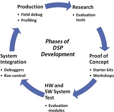
Figure 15-1: Phases of DSP development.
Challenges in DSP application development
The implementation of software for embedded digital signal processing applications is a very complex process. This complexity is a result of increasing functionality in embedded applications; intense time-to- market pressures; and very stringent cost, power, and speed constraints.
The primary goal for most DSP application algorithms focuses on the minimization of code size as well as the minimization of the memory required for the buffers that implement the main communication channels in the input dataflow. These are important problems because programmable DSPs have very limited amounts of on-chip memory, and the speed, power, and cost penalties for using off-chip memory are prohibitively high for many cost-sensitive embedded applications. Complicating the problem further, memory demands of applications are increasing at a significantly higher rate than the rate of increase in on-chip memory capacity offered by improved integrated circuit technology.
To help cope with such complexity, DSP system designers have increasingly been employing high-level, graphical design environments in which system specification is based on hierarchical dataflow graphs. Integrated development environments (IDE) are also being used in the program management and code build and debug phases of a project to manage increased complexity.
The main goal of this chapter is to explain the DSP application development flow and review the tools and techniques available to help the embedded DSP developer analyze, build, integrate, and test complex DSP applications.
Historically, digital signal processors have been programmed manually using assembly language. This is a tedious and error-prone process. A more efficient approach is to generate code automatically using available tooling. However, the auto-generated code must be efficient. DSPs have scarce amounts of on-chip memory and its use must be managed carefully. Using off-chip memory is inefficient due to increased cost, increased power requirements, and decreased speed penalty. All these drawbacks have a significant impact on real-time applications. Therefore, effective DSP-based code generation tools must specify the program in an imperative language such as C or C++ and use a good optimizing compiler.
The DSP design process
The DSP design process in many ways is similar to the standard software and system development process. However, the DSP development process also has some unique challenges that must be understood in order to develop efficient, high performance applications.
A high level model of the DSP system design process is shown in Figure 15-2. As shown in this figure, some of the steps in the DSP design process are similar to those found in the conventional system development process.
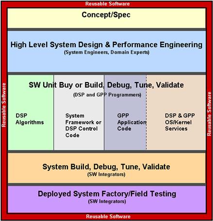
Figure 15-2: A block diagram of the general system design flow.
Concept and specification phase
The development of any signal processing system begins with the establishment of requirements for the system. In this step, the designer attempts to state the attributes of the system in terms of a set of requirements. These requirements should define the characteristics of the system expected by external observers such as users or other systems. This definition becomes the guide for all other decisions made during the design cycle.
DSP systems can have many types of the requirements that are common in other electronic systems. These requirements may include power, size, weight, bandwidth, and signal quality. However, DSP systems often have requirements that are unique to digital signal processing. Such requirements can include sample rate (which is related to bandwidth), data precision (which is related to signal quality), and real-time constraints (which are related to general system performance and functionality).
The designer devises a set of specifications for the system that describes the sort of system that will satisfy the requirements. These specifications are a very abstract design for the system. The process of creating specifications that satisfy the requirements is called requirements allocation.
A specification process for DSP systems
During the specification of the DSP system, using a real-time specification process such as Sommerville’s six-step real-time design process is recommended1. The six steps in this process include:
1. Identify the stimuli to be processed by the system and the required responses to these stimuli.
2. For each stimulus and response, identify the timing constraints. These timing constraints must be quantifiable.
3. Aggregate the stimulus and response processing into concurrent software processes. A process may be associated with each class of stimulus and response.
4. Design algorithms to process each class of stimulus and response. These must meet the given timing requirements. For DSP systems, these algorithms consist mainly of signal processing algorithms.
5. Design a scheduling system which will ensure that processes are started in time to meet their deadlines. The scheduling system is usually based on a pre-emptive multitasking model, using a rate monotonic or deadline monotonic algorithm.
6. Integrate using a real-time operating system (especially if the application is complex enough).
Once the stimuli and responses have been identified, a software function can be created by performing a mapping of stimuli to responses for all possible input sequences. This is important for real time systems. Any unmapped stimuli sequences can cause behavioral problems in the system.
Algorithm development and validation
During the concept and specification phase, a majority of the developer’s time is spent doing algorithm development. During this phase, the designer focuses on exploring approaches to solve the problems defined by the specifications at an abstract level. During this phase, the algorithm developer is usually not concerned with the details of how the algorithm will be implemented. Moreover, the developer focuses on defining a computational process which can satisfy the system specifications. The partitioning decisions of where the algorithms will be hosted (DSP, GPP, Hardware acceleration such as ASIC or FPGA) are not the number one concern at this time.
A majority of DSP applications require sophisticated control functions as well as complex signal processing functions. These control functions manage the decision-making and control flow for the entire application (for example, managing the various functional operations of a cell phone, as well as adjusting certain algorithm parameters based on user input). During this algorithm development phase, the designer must be able to specify as well as experiment with both the control behavior and the signal processing behavior of the application.
In many DSP systems, algorithm development first begins using floating-point arithmetic. At this point, there is no analysis or consideration of fixed-point effects resulting from running the application on a fixed point processor. Not that this analysis is not important. It is very critical to the overall success of the application and is considered shortly. But the main goal is to get an algorithm stream working, providing the assurance that the system can indeed work! When it comes to actually developing a productizable system, a less expensive fixed point processor may be the choice. During this time transition, the fixed point effects must be considered. In most cases it will be advantageous to implement the productizable system using simpler, smaller numeric formats with lower dynamic range to reduce system complexity and cost. This can only be found on fixed point DSPs.
For many kinds of applications, it is essential that system designers have the ability to evaluate candidate algorithms running in real-time, before committing to a specific design and hardware/software implementation. This is often necessary where subjective tests of algorithm quality are to be performed. For example, in evaluating speech compression algorithms for use in digital cellular telephones, real-time, two-way communications may be necessary.
DSP algorithm standards and guidelines
DSPs are often programmed like ‘traditional’ embedded microprocessors. They are programmed in a mix of C and assembly language, they directly access hardware peripherals, and for performance reasons, almost always have little or no standard operating system support. Thus, like traditional microprocessors, there is very little use of commercial off-the-shelf (COTS) software components for DSPs. However, unlike general-purpose embedded microprocessors, DSPs are designed to run sophisticated signal processing algorithms and heuristics. For example, they may be used to detect important data in the presence of noise, to or for speech recognition in a noisy automobile traveling at 65 miles per hour. Such algorithms are often the result of many years of research and development. However, because of the lack of consistent standards, it is not possible to use an algorithm in more than one system without significant reengineering. This can cause significant time to market issues for DSP developers. Appendix F provides more detail on DSP algorithm development standards and guidelines.
High level system design and performance engineering
High level system design refers to the overall partitioning, selection, and organization of the hardware and software components in a DSP system. The algorithms developed during the specification phase are used as the primary inputs to this partitioning and selection phase. Other factors are considered as well:
This phase is critical, as the designer must make trade-offs among these often conflicting demands. The goal is to select a set of hardware and software elements to create an overall system architecture that is well-matched to the demands of the application.
Modern DSP system development provides the engineer with a variety of choices to implement a given system. These include:
The designer must make the necessary system trade-offs in order to optimize the design to meet the system performance requirements that are most important (performance, power, memory, cost, manufacturability, etc.).
Performance engineering
Software performance engineering (SPE) aims to build predictable performance into systems by specifying and analyzing quantitative behavior from the very beginning of a system, through to its deployment and evolution. DSP designers must consider performance requirements, the design, and the environment in which the system will run. Analysis may be based on various kinds of modeling and design tools. SPE is a set of techniques for:
• Constructing a system performance model
• Evaluating the performance model
SPE requires the DSP developer to analyze the complete DSP system using the following information2:
• Workload; worst case scenarios
• Performance objectives; quantitative criteria for evaluating performance (CPU, memory, I/O)
• Software characteristics; processing steps for various performance scenarios (ADD, simulation)
• Execution environment; platform on which the proposed system will execute, partitioning decisions
• Resource requirements; estimate of the amount of service required for key components of the system
• Processing overhead; benchmarking, simulation, prototyping for key scenarios
Software development
Most DSP systems are developed using combinations of hardware components and software components. The proportion varies depending on the application (a system that requires fast upgradability or changeability will use more software; a system whose deploys mature algorithms and requires high performance may use hardware). Most systems based on programmable DSP processors are often software-intensive.
Software for DSP systems comes in many flavors. Aside from the signal processing software, there are many other software components required for programmable DSP solutions:
There is a growing trend towards the use of reusable or ‘off the shelf’ software components. This includes the use of reusable signal processing software components, application frameworks, operating systems and kernels, device drivers, and chip support software. DSP developers should take advantage of these reusable components whenever possible. The topic of reusable DSP software components is that of a later chapter.
System build, integration, and test
As DSP system complexity continues to grow, system integration becomes paramount. System integration can be defined as the progressive linking and testing of system components to merge their functional and technical characteristics into a comprehensive interoperable system. System integration is becoming more common in DSP systems can contain numerous complex hardware and software subsystems. It is common for these subsystems to be highly interdependent. System integration usually takes place throughout the design process. System integration may first be done using simulations prior to the actual fabrication of hardware.
System integration proceeds in stages as subsystem designs are developed and refined. Initially, much of the system integration may be performed on DSP simulators interfacing with simulations of other hardware and software components. The next level of system integration may be performed using a DSP evaluation board (this allows the software to be integraed with device drivers, board support packages, kernel, etc.). A final level of system integration can begin once the remaining hardware and software components are available.
Factory and field test
Factory and field test includes the remote analysis and debugging of DSP systems in the field or in final factory test. This phase of the lifecycle requires sophisticated tools which allow the field test engineer to quickly and accurately diagnose problems in the field and report those problems back to the product engineers to debug in a local lab.
Design challenges for DSP systems
What defines a DSP system are signal processing algorithms used in the application. These algorithms represent the numeric recipe for the arithmetic to be performed. However, the implementation decisions for these algorithms are the responsibility of the DSP engineer. The challenge for the DSP engineer is to understand the algorithms well enough to make intelligent implementation decisions what endure the computational accuracy of the algorithm while achieving ‘full technology entitlement’ for the programmable DSP in order to achieve the highest performance possible.
Many computationally intensive DSP systems must achieve very rigorous performance goals. These systems operate on lengthy segments of real-world signals that must be processed in real-time. These are hard real time systems that must always meet these performance goals, even under worst case system conditions. This is orders of magnitude more difficult than with a soft real time system where the deadlines can be missed occasionally.
DSPs are designed to perform certain classes of arithmetic operations such as addition and multiplication very quickly. The DSP engineer must be aware of these advantages and be able to use the numeric formats and type of arithmetic wisely to have a significant influence on the overall behavior and performance of the DSP system. One important choice is the selection of fixed-point or floating-point arithmetic. Floating-point arithmetic provides much greater dynamic range than does fixed-point arithmetic. Floating point also reduces the probability of overflow and the need for the programmer to worry about scaling. This alone can significantly simplify algorithm and software design, implementation, and test.
The drawback to floating-point processors (or floating point libraries) is that they are slower and more expensive than fixed-point. DSP engineers must perform the required analysis to understand the dynamic ranges needed throughput the application. It is highly probable that a complex DSP system will require different levels of dynamic range and precision at different points in the algorithm stream. The challenge is to perform the right amount of analysis in order to use the required numeric representations to achieve the performance required from the application.
In order to properly test a DSP system, a set of realistic test data is required. This test data may represent calls coming into a base station or data from another type of sensor that represents realistic scenarios. These realistic test signals are needed to verify the numeric performance of the system as well as the real-time constraints of the system. Some DSP applications must be tested for long periods of time in order to verify that there are no accumulator overflow conditions or other ‘corner cases’ that may degrade or break the system.
High level design tools for DSP
System-level design for DSP systems requires both high-level modeling to define the system concept and low level modeling to specify behavior details. The DSP system designer must develop complete end-to-end simulations and integrate various components such as analog and mixed signal, DSP, and control logic. Once the designer has modeled the system, the model must be executed and tested to verify performance to specifications. These models are also used to perform design trade-offs, what-if analysis, and system parameter tuning to optimize performance of the system.
DSP modeling tools exist to aid the designer in the rapid development of DSP-based systems and models. Hierarchical block-diagram design and simulation tools are available to model systems and simulate a wide range of DSP components. Application libraries are available for use by the designer that provide many of the common blocks found in DSP and digital communications systems. These libraries allow the designer to build complete end-to-end systems. Tools are also available to model control logic for event driven systems.
DSP toolboxes
DSP toolboxes are collections of signal processing functions that provide a customizable framework for both analog and digital signal processing. DSP toolboxes have graphical user interfaces that allow interactive analysis of the system. The advantage of these toolbox algorithms is that they are robust, reliable, and efficient. Many of these toolboxes allow the DSP developer to modify the supplied algorithm to more closely map to the existing architecture as well as the ability for the developer to add custom algorithms to the toolbox.
DSP system design tools also provide the capability for rapid design, graphical simulation, and prototyping of DSP systems. Blocks are selected from available libraries and interconnected in various configurations using point and click operations. Signal source blocks are used to test models. Simulations can be visualized interactively passed on for further processing. ANSI standard C code is generated directly from the model. Signal processing blocks, including FFT, DFT; window functions; decimation/interpolation; linear prediction; and multi-rate signal processing are available for rapid system design and prototyping.
Host development tools for DSP development
As mentioned earlier, there are many software challenges facing the real-time DSP developer:
A robust set of tools to aid the DSP developer can help speed development time, reduce errors, and more effectively manage large projects, among other advantages. Integrating a number of different tools into one integrated environment is called creating an Integrated Development Environment (IDE). An IDE is a programming environment that has been packaged as an application program. A typical IDE consists of a code editor, a compiler, a debugger, and a graphical user interface (GUI) builder. IDEs provide a user-friendly framework for building complex applications. PC developers first had access to IDEs.
Now applications are large and complex enough to warrant the same development environment for DSP applications. Currently, DSP vendors have IDEs to support their development environments. DSP development environments support some but not all of the overall DSP application development life cycle. As shown in Figure 15-3, the IDE is mainly used after the initial concept exploration, systems engineering, and partitioning phases of the development project. Development of the DSP application from inside the IDE mainly addressed software architecture, algorithm design and coding, the entire project build phase and the debug and optimize phases.
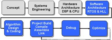
Figure 15-3: The DSP IDE is useful for some, but not all, of the DSP development life cycle.
A typical DSP IDE consists of several major components (Figure 15-4):
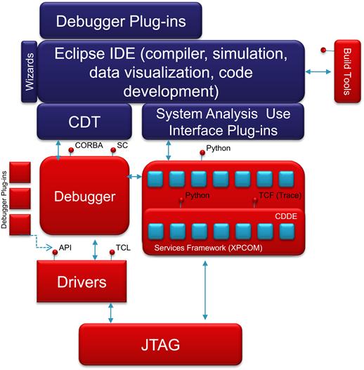
Figure 15-4: DSP integrated development environment.
A DSP IDE is optimized for DSP development. DSP development is different enough from other development to warrant a set of DSP-centric options within the IDE:
• Advanced real-time Debugging which includes advanced breakpoints, C-expression-based conditional breakpoints, and simultaneous view of source and dis-assembly
• Synchronized control over groups
• Probe points (advanced break points) provide oscilloscope-like functions
• File I/O with advanced triggering injects or extracts data signals
Data visualization, for example, allows the DSP developer to perform graphical signal analysis. This gives the developer the ability to view signals in native format and change variables on the fly to see their effects. You can read more about this topic in Chapter 17 on Developing and debugging DSP systems.
As DSP complexity grows and systems move from being cyclic executive to task based execution, more advanced tools are required to facilitate the integration and debug phase of development. DSP IDEs provide a robust set of ‘dashboards’ to help analyze and debug complex real-time applications. If more advanced task execution analysis is desired, a third party plug in capability can be used. For example, if the DSP developer needs to know why and where a task is blocked, not just if a task is blocked, rate monotonic analysis tools can be used to perform more detailed analysis.
DSP applications require real-time analysis of the system as it runs. DSP IDE’s provide the ability to monitor the system in real-time with low overhead and interference of the application. Because of the variety of real-time applications, these analysis capabilities are user controlled and optimized. Analysis data is accumulated and sent to the host in the background (a low priority non-intrusive thread performs this function, sending data over the JTAG interface to the host). These real-time analysis capabilities act as a software logic analyzer, performing tasks that, in the past, were performed by hardware logic analyzers. The analysis capability can show CPU load percentage (useful for finding hot spots in the application), the task execution history (to show the sequencing of events in the real-time system), a rough estimate of DSP MIPS (by using an idle counter), and the ability to log best and worst case execution times. This data can help the DSP developer determine whether the system is operating within its design specification, and meeting performance targets, and whether there are any subtle timing problems in the run time model of the system3.
System configuration tools allow the DSP developer to quickly prioritize system functions and perform what if analysis on different run time models.
The development tool flow starts from the most basic of requirements. The editor, assembler, and linker are, of course, are the most fundamental blocks. Once the linker has built an executable, there must be some way to load it into the target system. To do this, there must be run control of the target. The target can be a simulator (SIM), which is ideal for algorithm checkout when the hardware prototype is not available. The target can also be a starter kit (DSK) or an evaluation board (EVM) of some type. An evaluation board lets the developer run on real hardware, often with a degree of configurable I/O. Ultimately, the DSP developer will run the code on a prototype, and this requires an emulator.
Another important component of the IDE is the debugger. The debugger controls the simulator or emulator and gives the developer low level analysis and control of the program, memory, and registers in the target system. Because of the inherent nature of hardware/software co-design, the DSP developer must develop at least part of the application using a simulator instead of the real hardware.This means the DSP developer must debug systems without complete interfaces, or ones with I/O, but that don’t have real data available4. This is where file I/O helps the debug process. DSP debuggers generally have the ability to perform data capture as well as graphing capability in order to analyze the specific bits in the output file. Since DSP is all about code and application performance, it is also important to provide a way to measure code speed with the debugger (this is generally referred to as profiling). Finally, a real-time operating system capability allows the developer to build large complex applications and the Plug-In interface allows third parties (or the developer) to develop additional capabilities that integrate into the IDE.
A generic data flow example
This section will describe a simple example that brings together the various DSP development phases and tooling to produce a fully integrated DSP application. Figure 15-5 shows the simple model of a software system.
![]()
Figure 15-5: A generic data flow example.
Input is processed or transformed and output. From a real-time system perspective, the input will come from some sensor in the analog environment and the output will control some actuator in the analog environment. The next step will be to add data buffering to this model. Many real-time systems have a certain amount of input (and output) buffering to hold data while the CPU is busy processing a previous buffer of data. Figure 15-6 shows the example system with input and output data buffering added to the application.
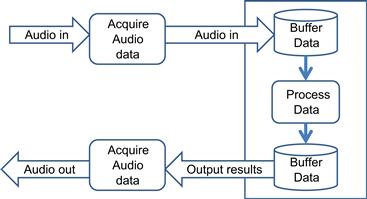
Figure 15-6: A data buffering model for a DSP application.
A more detailed model for data buffering is a double buffer model as shown in Figure 15-7. A double buffer is necessary because, as the CPU is busy processing one buffer, data from the external sensors must have a place to go and wait until the CPU has finished processing the current buffer of data. When the CPU finishes one buffer, it will begin processing the next buffer. The ‘old’ buffer (the buffer that was previously processed by the CPU) is now the current input buffer to hold data from the external sensors. When data is ready to be received (RCV ‘ping’ is empty, RCV flag = 1), RCV ‘pong’ buffer is emptied into the XMT ‘ping’ buffer (XMT flag = 0) for output & vice versa. This repeats continuously as data is input to and output from the system.
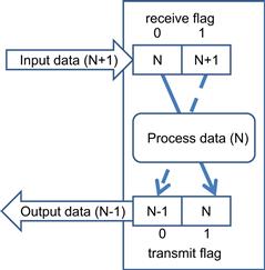
Figure 15-7: A data buffering model for processing real-time samples from the environment.
Analog data from the environment is input using the multi-channel buffered serial port interface. The external direct memory access controller (EDMA) manages the input of data into the DSP core and frees the CPU to perform other processing. The dual buffer implementation is realized in the on-chip data memory, which acts as the storage area. The CPU performs the processing on each of the buffers.
A combination of data in and data out views is shown in Figure 15-8. This is a system block diagram view shown mapped to a model of a DSP starter kit or evaluation board. The DSP starter kit in Figure 15-9 has a Codec which performs a transformation on the data before being sent to the buffered serial port and on into the DSP core using the DMA function. The DMA can be programmed to input data to either the Ping or Pong buffer and switch automatically so that the developer does not have to explicitly manage the dual buffer mechanism on the DSP.
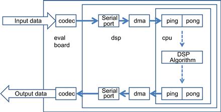
Figure 15-8: System block diagram of a DSP application mapped to a DSP starter kit.
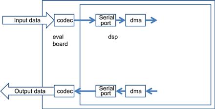
Figure 15-9: The peripheral processes required to get data in and out of the DSP on-chip memory.
In order to perform the coding for these peripheral processes, the DSP developer must perform the following steps:
• Direct DMA to continuously fill ping-pong buffers & interrupt CPU when full
• Select McBSP mode to match CODEC
The main software initialization processes and flow include:
The reset vectors operation performs the following tasks:
This is a device specific task that is manually managed.
Runtime support libraries are available to aid the DSP developer in developing DSP applications. This runtime software provides support for functions that are not part of the C language itself through inclusion of the following components:
• C I/O library – including printf()
• low-level support functions for I/O to the host operating system
• Intrinsic arithmetic routines
• System startup routine, _c_int00
• Functions and macros that allow C to access specific instructions
The main loop in this DSP application checks the buffer_data_ready_flag and calls the DSPBuffer() function when data is ready to be processed. The sample code for this is shown below.
void DSPBuffer(void)
void main( )
{
initialize_application( );
initialize_interrupts( );
while( true )
{
if(buffer_data_ready_flag)
{
buffer_data_ready_flag = 0;
DSPBuffer( );
Printf(“loop count = %d ”, i++);
}
}
}
Figure 15-10 shows how the link process maps the input files for the application to the memory map available on the hardware platform. Memory consists of various types including vectors for interrupts, code, stack space, global declarations, and constants.
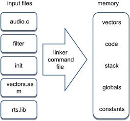
Figure 15-10: Mapping the input files to the memory map for the hardware requires a link process.
The link command file, LNK.CMD, is used to define the hardware and usage of the hardware by the input files. This allocation is shown in Figure 15-11. The MEMORY section lists the memory that the target system contains and the address ranges for those sections. This code is DSP device specific. The SECTIONS directive defines where the software components are to be placed in memory. Some section types include:
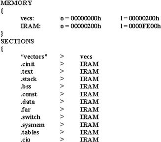
Figure 15-11: Sample code for the link command file mapping the input files to the target configuration.
The next step in our process is to set up the debugger target. Modern DSP IDEs support multiple hardware boards (usually within the same vendor family). Most of the setup can be done easily with drag and drop within the IDE. DSP developers can configure both DSP and non-DSP devices easily using the IDE.
DSP IDEs allow projects to be visually managed. Component files are placed into the project easily using drag and drop. Dependency listings are also maintained automatically. Project management is supported in DSP IDEs and allow easy configuration and management of a large number of files in a DSP application.
The plug in capability provided by DSP IDEs allows the DSP developer to customize the development environment to the specific needs of the application and developer. Within the development environment, the developer can customize the input and output devices to be used to input and analyze data, respectively. Block diagram tools and custom editors and build tools can be used with the DSP IDE to provide valuable extensions to the development environment.
Debug – verifying code performance
DSP IDEs also support the debug stage of the software development life cycle. During the phase, the first goal is to verify the system is logically correct. In the example being discussed, this phase is used to insure that the filter operates properly on the audio input signal. During this phase, the following steps can be performed in the IDE to set up and run the system to verify the logical correctness of the system:
• Load program to the target DSP
• Run to ‘main()’ or other functions
• Set and run to Breakpoints to halt execution at any point
• Display data in Graphs for visual analysis of signal data
The debug phase is also used to verify that the temporal or real-time goals of the system are being met. During this phase, the developer determines if the code is running as efficiently as possible and if the execution time overhead is low enough without sacrificing the algorithm fidelity. Probe points inserted in the tool can be used in conjunction with visual graphing tools; this is helpful during this phase to verify both the functional as well as temporal aspects of the system. The visual graphs are updated each time the probe point is encountered in the code.
Code tuning and optimization
One of the main differentiators between developers of non-real-time systems and real-time systems is the phase of code tuning and optimization. It is during this phase that the DSP developer looks for ‘hot spots’ or inefficient code segments and attempts to optimize those segments. Code in real-time DSP systems are often optimized for speed, memory size, or power. DSP code build tools (compilers, assemblers, and linkers) are improving to the point where developers can write a majority, if not all, of their application in high level language like C or C++.
Nevertheless, the developer must provide help and guidance to the compiler in order to get the technology entitlement from the DSP architecture. DSP compilers perform architecture specific optimizations and provide the developer with feedback on the decisions and assumptions that were made during the compile process. The developer must iterate in this phase to address the decisions and assumptions made during the build process until the performance goals are met. DSP developers can give the DSP compiler specific instructions using a number of compiler options. These options direct the compiler as to the level of aggressiveness to use when compiling the code, whether to focus on code speed or size, whether to compile with advanced debug information, and many other options.
Given the potentially large number of degrees of freedom in compile options and optimization axes (speed, size, power), the number of tradeoffs available during the optimization phase can be enormous (especially considering that every function or file in an application can be compiled with different options). Profile based optimization can be used to graph a summary of code size versus speed options. The developer can choose the option that meets the goals for speed and power and have the application automatically built with the options that yield the selected size/speed tradeoff selected.
Typical DSP development flow
DSP developers follow a development flow that takes them through several phases:
• Application definition; it is during this phase that the developer begins to focus on the end goals for performance, power, and cost
• Architecture design; during this phase, the application is designed at a systems level using block diagrams and signal flow tools if the application is large enough to justify using these tools
• Hardware / software mapping; in this phase a target decision is made for each block and signal in the architecture design
• Code creation; this phase is where the initial development is done, prototypes are developed and mockups of the system are performed
• Validate / debug; functional correctness is verified during this phase
• Tuning / optimization; this is the phase where the developer’s goal is to meet the performance goals of the system
Developing a well tuned and optimized application involves several iterations between the validate phase and the optimize phase. Each time through the validate phase the developer will edit and build the modified application, run it on a target or simulator, and analyze the results for functional correctness. Once the application is functionally correct, the developer will begin a phase of optimization on the functionally correct code. This involves tuning the application towards the performance goals of the system (speed, memory, power, for example), running the tuned code on the target or simulator to measure the performance, and evaluation where the developer will analyze the remaining ‘hot spots’ or areas of concern that have not yet been addressed, or are still outside the goals of performance for that particular area (Figure 15-12).
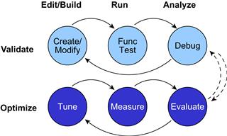
Figure 15-12: DSP developers iterate through a series of optimize and validate steps until the goals for performance are achieved.
Once the evaluation is complete, the developer will go back to the validate phase where the new, more optimized code is run to verify functional correctness has not been compromised. If not, and the performance of the application is within acceptable goals for the developer, the process stops. If a particular optimization has broken the functional correctness of the code, the developer will debug the system to determine what has been broken, fix the problem, and continue with another round of optimization. Optimizing DSP applications inherently leads to more complex code, and the likelihood of breaking something that used to work increases, the more aggressively the developer optimizes the application. There can be many cycles in this process, continuing until the performance goals have been met for the system.
Generally, a DSP application will initially be developed without much optimization. During this early period, the DSP developer is primarily concerned with functional correctness of the application. Therefore, the ‘out of box’ experience from a performance perspective is not that impressive, even when using the more aggressive levels of optimization in the DSP compiler.
This initial view can be termed the ‘pessimistic’ view in the sense that there are no aggressive assumptions made in the compiled output, there is no aggressive mapping of the application to the specific DSP architecture, and there is no aggressive algorithmic transformation to allow the application to run more efficiently on the target DSP.
Significant performance improvements can come quickly by focusing on a few critical areas of the application:
• Key tight loops in the code with many iterations
The techniques to perform these optimizations were discussed in the chapter on optimizing DSP software. If these few key optimizations are performed, the overall system performance goes up significantly. As Figure 15-13 shows, a few key optimizations on a small percentage of the code early, leads to significant performance improvements. Additional phases of optimization get more and more difficult as the optimization opportunities are reduced as well as the cost/benefit of each additional optimization.
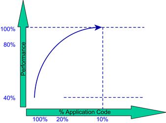
Figure 15-13: Optimizing DSP code takes time and effort to reach the desired performance goals.
The goal of the DSP developer must be to continue to optimize the application until the performance goals of the system are met, not until the application is running at its theoretical peak performance. The cost / benefit does not justify this approach.
After each optimization, the profiled application can be analyzed for where the majority of cycles or memory is being consumed by the application. DSP IDEs provide advanced profiling capabilities that allow the DSP developer to profile the application and display useful information about the application such as code size, total cycle count, number of times the algorithm looped through a particular function, etc. This information can then be analyzed to determine which functions are optimization candidates.
An optimal approach to profiling and tuning a DSP application is to attack the right areas first. These represent those areas where the most performance improvement can be gained with the smallest effort. A Pareto ranking of the biggest performance areas (Figure 15-14) will guide the DSP developer towards those areas where the most performance can be gained.
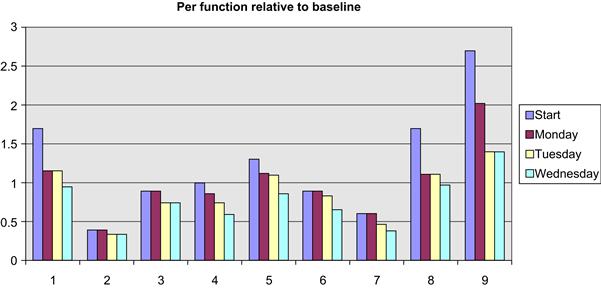
Figure 15-14: A pareto analysis of a DSP function allows the DSP developer to focus on the most important areas first.
Getting started
A DSP starter kit is easy to install and allows the developer to get started writing code very quickly. The starter kits usually come with a daughter card expansion slots, the target hardware, software development tools, a parallel port interface for debug, a power supply, and the appropriate cables.
An evaluation module is more complex and is used for more in depth analysis of an application space. Evaluation modules have more advanced hardware and software to support this analysis and evaluation.
Putting it all together
Figure 15-15 shows the entire DSP development flow. There are five major stages to the DSP development process:
• System concept and requirements; this phase includes the elicitation of the system level functional and non-functional (sometimes called ‘quality’) requirements. Power requirements, Quality of Service (QoS), performance, and other system level requirements are elicited. Modeling techniques like signal flow graphs are constructed to examine the major building blocks of the system.
• System algorithm research and experimentation; during this phase, the detailed algorithms are developed based on the given performance and accuracy requirements. Analysis is first done on floating point development systems to determine if these performance and accuracy requirements can be met. These system are then ported, if necessary, to fixed point processors for cost reasons. Inexpensive evaluation boards are used for this analysis.
• System design; during the design phase, the hardware and software blocks for the system are selected and/or developed. These systems are analyzed using prototyping and simulation to determine if the right partitioning has been performed and whether the performance goals can be realized using the given hardware and software components. Software components can be custom developed or reused, depending on the application.
• System implementation; during the system implementation phase, inputs from system prototyping, trade off studies, and hardware synthesis options are used to develop a full system co-simulation model. Software algorithms and components are used to develop the software system. Combinations of signal processing algorithms and control frameworks are used to develop the system.
• System integration; during the system integration phase, the system is built, validated, tuned if necessary and executed in a simulated environment or in a hardware in the loop simulation environment. The scheduled system is analyzed and potentially re-partitioned if performance goals are not being met.
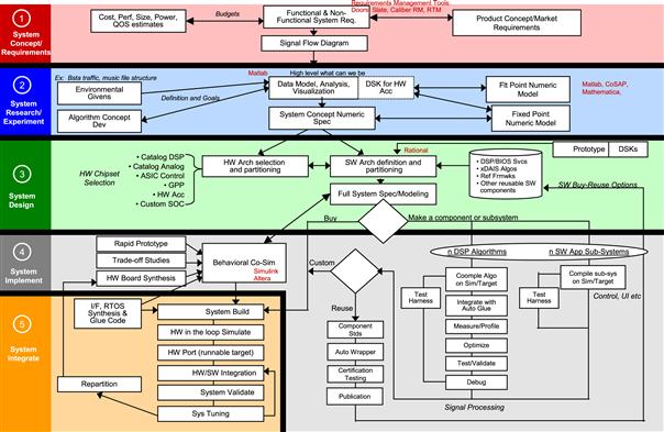
Figure 15-15: The DSP development flow.
In many ways, the DSP system development process is similar to other development processes. Given the increased amount of signal processing algorithms, early simulation-based analysis is required more for these systems. The increased focus on performance requires the DSP development process to focus more on real-time deadlines and iterations of performance tuning. We have discussed some of the details of these phases throughout this book.
1 Software Engineering version 9 by Ian Sommerville, chapter 16.
2 See Performance Solutions as an excellent reference to this technology
3 If you can’t see the problem, you can’t fix the problem
4 A case study of the hardware/software co-design as well as the analysis techniques for embedded DSP and micro devices is at the end of the chapter.