
Chapter 3. The CUDA Tool Suite
Profiling a PCA/NLPCA Functor
CUDA enables efficient GPGPU computing with just a few simple additions to the C language. Simplicity of expression, however, does not equate to simplicity of program execution. As when developing applications for any computer, identifying performance bottlenecks can be complicated. Following the same economy of change used to adapt C and C++, NVIDIA has extended several popular profiling tools to support GPU computing. These are tools that most Windows and UNIX developers are already proficient and comfortable using such as gprof and Visual Studio. Additional tools such as hardware-level GPU profiling and a visual profiler have been added. Those familiar with building, debugging, and profiling software under Windows and UNIX should find the transition to CUDA straight-forward. All CUDA tools are freely available on the NVIDIA website including the professional edition of Parallel Nsight for Microsoft Visual Studio.
Keywords
Profiling, Principle Components, PCA, NLPCA, data-mining, Visual profiler, Parallel Nsight
CUDA enables efficient GPGPU computing with just a few simple additions to the C language. Simplicity of expression, however, does not equate to simplicity of program execution. As when developing applications for any computer, identifying performance bottlenecks can be complicated. Following the same economy of change used to adapt C and C++, NVIDIA has extended several popular profiling tools to support GPU computing. These are tools that most Windows and UNIX developers are already proficient and comfortable using such as gprof and Visual Studio. Additional tools such as hardware-level GPU profiling and a visual profiler have been added. Those familiar with building, debugging, and profiling software under Windows and UNIX should find the transition to CUDA straight-forward. All CUDA tools are freely available on the NVIDIA website including the professional edition of Parallel Nsight for Microsoft Visual Studio.
In this chapter, the Microsoft and UNIX profiling tools for CUDA will be used to analyze the performance and scaling of the Nelder-Mead optimization technique when optimizing a PCA and NLPCA functor.
At the end of the chapter, the reader will have a basic understanding of:
■ PCA and NPLCA analysis, including the applicability of this technique to data mining, dimension reduction, feature extraction, and other data analysis and pattern recognition problems.
■ How the CUDA profiling tools can be used to identify bottlenecks and scaling issues in algorithms.
■ Scalability issues and how even a simple dynamic memory allocation can have dramatic performance implications on an application.
PCA and NLPCA
Principle Components Analysis (PCA) is extensively used in data mining and data analysis to (1) reduce the dimensionality of a data set and (2) extract features from a data set. Feature extraction refers to the identification of the salient aspects or properties of data to facilitate its use in a subsequent task, such as regression or classification (Duda & Hart, 1973). Obviously, extracting the principal features of a data set can help with interpretation, analysis, and understanding.
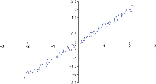
PCA analysis accounts for the maximum amount of variance in a data set using a set of straight lines where each line is defined by a weighted linear combination of the observed variables. The first line, or principle component, accounts for the greatest amount of variance; each succeeding component accounts for as much variance as possible while remaining orthogonal to (uncorrelated with) the preceding components. For example, a cigar-shaped distribution would require a single line (or principal component) to account for most of the variance in the data set illustrated in Figure 3.1.
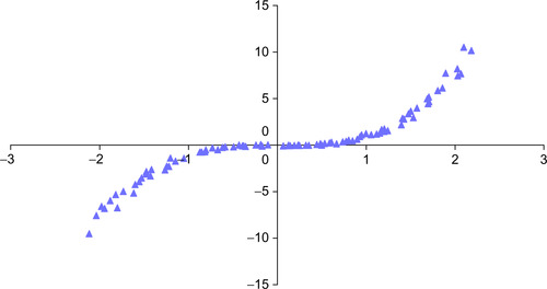
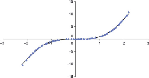
PCA utilizes straight lines; NLPCA can utilize continuous open or closed curves to account for variance in data (Hsieh, 2004). A circle is one example of a closed curve that joins itself so there are no end points. Figure 3.2 illustrates an open curve. As a result, NLPCA has the ability to represent nonlinear problems in a lower dimensional space. Figure 3.2 illustrates one data set in which a single curve could account for most of the variance.
NLPCA has wide applicability to numerous challenging problems, including image and handwriting analysis (Hinton & Salakhutdinov, 2006; Schölkopf & Klaus-Robert Müller, 1998) as well as biological modeling (Scholz, 2007), climate (Hsieh, 2001; Monahan, 2000), and chemistry (Kramer, 1991). Geoffrey E. Hinton has an excellent set of tutorials on his website at the University of Toronto (Hinton, 2011). Chapter 10 expands this use of MPI (Message Passing Interface) so that it can run across hundreds of GPUs. Chapter 12 provides a working framework for real-time vision analysis that can be used as a starting point to explore these and more advanced techniques.
Autoencoders
In 1982, Erkki Oja proposed the use of a restricted number of linear hidden neurons, or bottleneck neurons, in a neural network to perform PCA analysis (Oja, 1982). Figure 3.3 illustrates a simple linear network with two inputs and one hidden neuron.
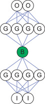
Such networks were later generalized to perform NLPCA. Figure 3.1 illustrates an architecture recommended by Kramer (1991) that uses multiple hidden layers with a sigmoidal nonlinear operator. The bottleneck neuron can be either linear or nonlinear. Hsieh extended this architecture to closed curves by using a circular node at the bottleneck (2001).
During training, the ANN essentially teaches itself because the input vectors are utilized as the known output vectors, which forces the lower half of the network to transform each input vector from a high- to low-dimensional space (from two dimensions to one in Figure 3.4) in such a way that the upper half of the network can correctly reconstruct the original high-dimensional input vector at the output neurons. A least-means-squared error is commonly used to determine the error over all the vectors. Such networks are sometimes called autoencoders. A perfect encoding would result in a zero error on the training set, as each vector would be exactly reconstructed at the output neurons. During analysis, the lower half of the network is used to calculate the low-dimensional encoding. Autoencoders have been studied extensively in the literature (Hinton & Salakhutdinov, 2006; Kramer, 1991) and are part of several common toolkits including MATLAB. One example is the nlpca toolkit on nlpca.org.
An Example Functor for PCA Analysis
Example 3.1, “A PCA Functor Implementing the Network in Figure 3.3,” demonstrates the simplicity of the functor that describes the PCA network illustrated in Figure 3.3. This functor is designed to be substituted into the Nelder-Mead optimization source code from Chapter 2, which contains the typename definition for Real and variables used in this calculation.
static const int nInput = 2;
static const int nH1 = 1;
static const int nOutput = nInput;
static const int nParam =
(nOutput+nH1) // Neuron Offsets
+ (nInput*nH1) // connections from I to H1
+ (nH1*nOutput); // connections from H1 to O
static const int exLen = nInput;
struct CalcError {
const Real* examples;
const Real* p;
const int nInput;
const int exLen;
CalcError( const Real* _examples, constReal* _p,
const int _nInput, const int _exLen)
: examples(_examples), p(_p), nInput(_nInput), exLen(_exLen) {};
__device__ __host__
Real operator()(unsigned int tid)
{
const register Real* in = &examples[tid * exLen];
register int index=0;
register Real h0 = p[index++];
for(int i=0; i < nInput; i++) {
register Real input=in[i];
h0 += input * p[index++];
}
register Real sum = 0.;
for(int i=0; i < nInput; i++) {
register Real o = p[index++];
o += h0 * p[index++];
o −= in[i];
sum += o*o;
}
return sum;
}
};
Example 3.2, “A Linear Data Generator,” defines the subroutine genData(), which creates a two-dimensional data set based on the linear relationship between two variables z1 and z2 shown in Equation 3.1. Noise is superimposed onto t according to two uniformly distributed sequences, e1 and e2 with zero mean. A variance of 0.1 was used to generate the training data and for Figure 3.1.
template <typename Real>
void genData(thrust::host_vector<Real> &h_data, int nVec, Real xVar)
{
Real xMax = 1.1; Real xMin = −xMax;
Real xRange = (xMax − xMin);
for(int i=0; i < nVec; i++) {
Real t = xRange * f_rand();
Real z1 = t +xVar * f_rand();
Real z2 = t +xVar * f_rand();
h_data.push_back( z1 );
h_data.push_back( z2 );
}
}
(3.1)
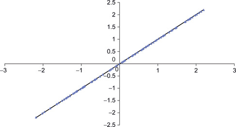
Figure 3.5 shows how the PCA network was able to reconstruct 100 randomly generated data points using genData with a zero variance (xVar equals zero).
The complete source code for this example can be downloaded from the book's website. Those who wish to adapt the xorNM.cu example from Chapter 2 can use the functor in Example 3.1 and data generator in Example 3.2. In addition, the test for correctness will need to be modified. To attain high-accuracy, this example required that kcount be set to 50000.
An Example Functor for NLPCA Analysis
The NLPCA functor in Example 3.3 implements the network shown in Figure 3.4. This functor is designed to be substituted into the Nelder-Mead optimization source code from Chapter 2, which contains the typename definition for Real and variables used in this calculation.
static const int nInput = 2;
static const int nH1 = 4;
static const int nH2 = 1;
static const int nH3 = 4;
static const int nOutput = nInput;
static const int nParam =
(nOutput+nH1+nH2+nH3) // Neuron Offsets
+ (nInput*nH1)// connections from I to H1
+ (nH1*nH2)// connections from H1 to H2
+ (nH2*nH3)// connections from H2 to H3
+ (nH3*nOutput); // connections from H3 to O
static const int exLen = nInput;
struct CalcError {
const Real* examples;
const Real* p;
const int nInput;
const int exLen;
CalcError( const Real* _examples, constReal* _p,
const int _nInput, const int _exLen)
: examples(_examples), p(_p), nInput(_nInput), exLen(_exLen) {};
__device__ __host__
Real operator()(unsigned int tid)
{
const register Real* in = &examples[tid * exLen];
register int index=0;
register Real h2_0 = p[index++]; // bottleneck neuron
{
register Real h1_0 = p[index++];
register Real h1_1 = p[index++];
register Real h1_2 = p[index++];
register Real h1_3 = p[index++];
for(int i=0; i < nInput; i++) {
register Real input=in[i];
h1_0 += input * p[index++]; h1_1 += input * p[index++];
h1_2 += input * p[index++]; h1_3 += input * p[index++];
}
h1_0 = G(h1_0); h1_1 = G(h1_1);
h1_2 = G(h1_2); h1_3 = G(h1_3);
h2_0 += p[index++] * h1_0; h2_0 += p[index++] * h1_1;
h2_0 += p[index++] * h1_2; h2_0 += p[index++] * h1_3;
}
register Real h3_0 = p[index++];
register Real h3_1 = p[index++];
register Real h3_2 = p[index++];
register Real h3_3 = p[index++];
h3_0 += p[index++] * h2_0; h3_1 += p[index++] * h2_0;
h3_2 += p[index++] * h2_0; h3_3 += p[index++] * h2_0;
h3_0 = G(h3_0); h3_1 = G(h3_1);
h3_2 = G(h3_2); h3_3 = G(h3_3);
register Real sum = 0.;
for(int i=0; i < nOutput; i++) {
register Real o = p[index++];
o += h3_0 * p[index++]; o += h3_1 * p[index++];
o += h3_2 * p[index++]; o += h3_3 * p[index++];
o −= in[i];
sum += o*o;
}
return sum;
}
};
The genData method is modified to define a nonlinear relationship between z1 and z2 with e1 and e2 as described previously for the PCA data generator. Example 3.4 implements a nonlinear data generator using Equation 3.2.
(3.2)
template <typename Real>
void genData(thrust::host_vector<Real> &h_data, int nVec, Real xVar)
{
Real xMax = 1.1; Real xMin = -xMax;
Real xRange = (xMax - xMin);
for(int i=0; i < nVec; i++) {
Real t = xRange * f_rand();
Real z1 = t +xVar * f_rand();
Real z2 = t*t*t +xVar * f_rand();
h_data.push_back( z1 );
h_data.push_back( z2 );
}
}
Figure 3.6 shows that the network found a reasonable solution with a bottleneck of one neuron. The scatterplot reconstructs the high-dimensional data for 100 randomly chosen points on the curve.
The complete source code can be downloaded from the book's website.
Obtaining Basic Profile Information
The collection of low-level GPU profiling information can be enabled through use of the environmental variable CUDA_PROFILE. Setting this variable to 1 tells CUDA to collect runtime profiling information from hardware counters on the GPU. Gathering this information does not require special compiler flags, nor does it affect application performance. Setting CUDA_PROFILE to 0 disables the collection of the profile information.
By default, the CUDA profiler writes information to the file cuda_profile_0.log in the current directory. The name of the destination file can be changed through the environment variable CUDA_PROFILE_LOG. Further, the user can specify an options file to select the specific information that is to be gathered from the hardware counters with the environmental variable CUDA_PROFILE_CONFIG. The types and amounts of profile information that can be collected differ between GPU generations. Please consult the NVIDIA profiler documentation to see what information can be gathered from your GPGPU.
Examining the contents of cuda_profile_0.log after running nlpcaNM_GPU32 with CUDA_PROFILE=1 shows that indeed this is the raw profiler output. Just looking at the first few lines, one can see that several data transfers occurred from the host to device after the application started, which we can infer are the movement of the training set, parameters, and other information to the GPGPU. Highlighted in Example 3.5, “CUDA GPU Profile for Single-Precision Nelder-Mead NLPCA Optimization,” is a reported occupancy value, which is a measure of GPU thread-level parallelization (TLP). High occupancy is generally good, but high application performance can also be achieved by applications with lower occupancy that attain high instruction-level parallelism (ILP). To understand occupancy, you need to understand some basics about the GPU hardware and execution model as discussed in the next chapter.
# CUDA_PROFILE_LOG_VERSION 2.0
# CUDA_DEVICE 0 Tesla C2070
# TIMESTAMPFACTOR fffff6faa0f3f368
method,gputime,cputime,occupancy
method=[ memcpyHtoD ] gputime=[ 1752.224 ] cputime=[ 1873.000 ]
method=[ memcpyDtoD ] gputime=[ 179.296 ] cputime=[ 20.000 ]
method=[ _ZN6thrust6detail6device4cuda6detail23launch_closure_by_valueINS2_18for_each_n_closureINS_10device_ptrIyEEjNS0_16generate_functorINS0_12fill_functorIyEEEEEEEEvT_ ] gputime=[ 5.056 ] cputime=[ 7.000 ] occupancy=[ 0.500 ]
method=[ _ZN6thrust6detail6device4cuda6detail23launch_closure_by_valueINS2_18for_each_n_closureINS_10device_ptrIfEEjNS0_16generate_functorINS0_12fill_functorIfEEEEEEEEvT_ ] gputime=[ 2.144 ] cputime=[ 5.000 ] occupancy=[ 0.500 ]
method=[ memcpyDtoD ] gputime=[ 2.048 ] cputime=[ 5.000 ]
method=[ memcpyHtoD ] gputime=[ 1.120 ] cputime=[ 5.000 ]
method=[ memcpyHtoD ] gputime=[ 1.088 ] cputime=[ 3.000 ]
method=[ _ZN6thrust6detail6device4cuda6detail23launch_closure_by_valueINS3_21reduce_n_smem_closureINS_18transform_iteratorIN7ObjFuncIfE9CalcErrorENS_17counting_iteratorIjNS_11use_defaultESB_ SB_EEfSB_EElfNS_4plusIfEEEEEEvT_ ] gputime=[ 850.144 ] cputime= [ 5.000 ] occupancy=[ 0.625 ]
method=[ _ZN6thrust6detail6device4cuda6detail23launch_closure_by_valueINS3_21reduce_n_smem_closureINS0_15normal_iteratorINS_10device_ptrIfEEEElfNS_4plusIfEEEEEEvT_ ] gputime=[ 5.952 ] cputime=[ 4.000 ] occupancy=[ 0.500 ]
method=[ memcpyDtoH ] gputime=[ 1.952 ] cputime=[ 856.000 ]
method=[ memcpyHtoD ] gputime=[ 1.120 ] cputime=[ 4.000 ]
method=[ memcpyHtoD ] gputime=[ 1.088 ] cputime=[ 4.000 ]
...
Gprof: A Common UNIX Profiler
To gain insight into host side performance, a CUDA application can be compiled with the -profile command-line option as seen in the nvcc command in Example 3.6:
nvcc --profile -arch=sm_20 -O3 -Xcompiler -fopenmp nlpcaNM.cu
The Linux gprof profiler can then be used to examine the host-side behavior. The following output shows that the Nelder-Mead optimization method nelmin (highlighted in the following example), consumed only 10.79% of the runtime. The next largest consumer of host-only time is the allocation of the four STL (Standard Template library) vectors in nelmin() aside from two host-side methods supporting thrust on the GPU. Gprof reports that nelmin() is only called once, allowing us to conclude that the Nelder-Mead optimization code does not make significant demands on the host processor. See Example 3.7, “Example gprof Output”:
Flat profile:
Each sample counts as 0.01 seconds.
%cumulativeselfselftotal
timesecondssecondscallss/calls/callname
10.790.220.2210.221.08void nelmin <float>(float (*)(float*), int, float*, float*, float*, float, float*, int, int, int*, int*, int*)
9.800.420.20105088800.000.00unsigned long thrust::detail::util::divide_ri<unsigned long, unsigned long>(unsigned long, unsigned long)
8.330.590.1735029600.000.00thrust:: detail::device::cuda::arch::max_active_blocks_per_multiprocessor(cudaDeviceProp const&, cudaFuncAttributes const&, unsigned long, unsigned long)
4.410.680.09120011440.000.00void thrust::advance<thrust::detail::normal_iterator<float*>, unsigned long>(thrust::detail::normal_iterator<float*>&, unsigned long)
3.920.760.08697305620.000.00std:: vector<float, std::allocator<float> >::operator[](unsigned long)
...
The combined output of both the CUDA profiler and gprof demonstrate that the optimization functor dominates the runtime of this application. Although much useful information can be gathered with gprof and the CUDA profiler, it still takes considerable work and some guesswork to extract and analyze the information.
More information about can be found in the gprof manual. The NVIDIA documentation on the visual profiler is an excellent source of information about the low-level CUDA profiler.
The NVIDIA Visual Profiler: Computeprof
NVIDIA provides the visual profiler computeprof for UNIX, Windows, and Mac to collect and analyze the low-level GPU profiler output for the user. As with the low-level profiler, the application does not need to be compiled with any special flags. By default, the visual profiler runs the application 15 times for 30 seconds per run to gather an ensemble of measurements.
The visual profiler is simple to use:
■ Launch the CUDA visual profiler using the computeprof command.
■ In the dialog that comes up, press the “Profile application” button in the “Session” pane.
■ In the next dialog that comes up, type in the full path to your compiled CUDA program in the “Launch” text area.
■ Provide any arguments to your program in the “Arguments” text area. Leave this blank if your code doesn't take any arguments.
■ Make sure the “Enable profiling at application launch” and “CUDA API Trace” settings are checked.
■ Press the “Launch” button at the bottom of the dialog to begin profiling.
Table 3.1 shows the information presented by default on the visual profiler summary screen after profiling the binary for nlpcaNM.cu.
Thrust generates some obscure names, but we can infer that launch_closure_by_value-2 is transform_reduce performing a transform with the CalcError functor. The launch_closure_by_value-3 method is the following reduction operation. The number of transform and reduce operations should be the same. We can infer that the different number of calls in the report (58 vs. 57) was caused by termination of the application by the visual profiler after 30 seconds of runtime.
According to the three rules of efficient GPGPU programming introduced in Chapter 1, Table 3.1 shows that our application is very efficient:
1. Get the data on the GPGPU and keep it there.
This application is not limited by PCIe bus speed, as less than 4% of the runtime is consumed by the combined data transfer operations (memcpyHtoD(), memcpyDtoD(), and memcpyDtoH()).
2. Give the GPGPU enough work to do.
This application is not bound by kernel startup legacy, as the dominant method consumes 83.38% of the runtime and takes an average 49,919 microseconds to complete—far beyond the nominal kernel startup time of four microseconds.
3. Focus on data reuse within the GPGPU to avoid memory bandwidth limitations.
The runtime is dominated by a method that has an instructions per clock count (IPC) of 1.77, which is close to the peak theoretical limit of two instructions per clock for a 20-series Fermi GPGPU like the C2070. Further, this kernel is not limited by memory bandwidth, as the global memory bandwidth usage of 10.63 GB/s is less than 10% of the 143 GB/s the C2070 memory subsystem can provide. Further the l1 gld (Global Load) hit rate shows that the cache is being utilized effectively 94% of the time.
The visual profiler will automatically perform much of the preceding analysis for the user by clicking on a method name in the Method field. The report in Example 3.8, “Visual Profiler Kernel Analysis,” was generated after clicking on launch_closure_by_value-2:
Analysis for kernel launch_closure_by_value-2 on device Tesla C2070
Summary profiling information for the kernel:
Number of calls:58
Minimum GPU time(us):794.37
Maximum GPU time(us):951.78
Average GPU time(us):860.68
GPU time (%):83.86
Grid size:[1411]
Block size:[96011]
Limiting Factor
Achieved Instruction Per Byte Ratio:45.92 ( Balanced Instruction Per Byte Ratio: 3.58 )
Achieved Occupancy:0.63 ( Theoretical Occupancy: 0.62 )
IPC:1.77 ( Maximum IPC: 2 )
Achieved global memory throughput:10.71 ( Peak global memory throughput(GB/s): 143.42 )
Hint(s)
The achieved instructions per byte ratio for the kernel is greater than the balanced instruction per byte ratio for the device. Hence, the kernel is likely compute bound. For details, click on Instruction Throughput Analysis.
Clicking the “Instruction Throughput Analysis” button shows that this kernel is indeed achieving a very high instruction throughput. There is some branching in the kernel that most likely happens inside the tanh() function, which suggests using another sigmoidal function to increase performance. See Example 3.9, “Visual Profiler Instruction Analysis”:
IPC: 1.77
Maximum IPC: 2
Divergent branches(%): 13.47
Control flow divergence(%): 12.62
Replayed Instructions(%): 1.08
Global memory replay(%): 0.55
Local memory replays(%): 0.00
Shared bank conflict replay(%): 0.00
Shared memory bank conflict per shared memory instruction(%): 0.00
The NVIDIA visual profiler (computeprof) collects and provides a wealth of additional information and analysis not discussed here. The Visual Profiler manual is an excellent source of information, 1 as is the help tab on the startup screen. Just type computeprof and click on help in the GUI. Later chapters will reference important computeprof profiler measurements to aid in the understanding and interpretation of GPU performance. Because the Visual Profiler runs on all CUDA-enabled operating systems (Windows, UNIX, and Mac OS X), these discussions should benefit all readers.
1Downloadable along with CUDA at http://developer.nvidia.com/cuda-downloads.
Parallel Nsight for Microsoft Visual Studio
Parallel Nsight is the debugging and analysis tool that NVIDIA provides for Microsoft developers; it installs as a plug-in within Microsoft Visual Studio. Parallel Nsight allows both debugging and analysis on the machine as well as on remote machines, which can be located at a customer's site. Be aware that the capabilities of Parallel Nsight vary with the hardware configuration, as can be seen in Table 3.2.
The following discussion highlights only a few features of Parallel Nsight as part of our analysis of nlpcaNM.cu. Parallel Nsight is an extensive package that is growing and maturing quickly. The most current information—including videos and user forums—can be found on the Parallel Nsight web portal (http://www.nvidia.com/ParallelNsight) as well as in the help section in Visual Studio.
The Nsight Timeline Analysis
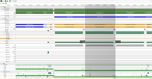
As can be seen in Trace timeline in Figure 3.7, Parallel Nsight provides a tremendous amount of information that is easily accessible via mouseover and zooming operations, as well as various filtering operations. Given the volume of information available in these traces, it is essential to know that regions of the timeline can be selected by clicking the mouse on the screen at a desired starting point of time. A vertical line will appear on the screen. Then press the Shift key and move the mouse (with the button pressed) to the end region of interest. This action will result in a gray overlay, as shown in Figure 3.7. A nice feature is that the time interval for the region is calculated and displayed.
The timeline can be used to determine if the application is CPU-bound, memory-bound, or kernel-bound:
■ CPU-bound: There will be large areas where the kernel is shown to be running.
■ PCIe transfer–limited: Kernel execution is blocked while waiting on memory transfers to or from the device, which can be seen by looking at the Memory row. If much time is being spent waiting on memory copies, consider using the Streams API to pipeline the application. This API allows data transfers and kernel execution to overlap. Before modifying code, compare the duration of the transfers and kernels to ensure that a performance gain will be realized.
■ Kernel-bound: If the majority of the application time is spent waiting on kernels to complete, then switch to the “Profile CUDA” activity and rerun the application to collect information from the hardware counters. This information can help guide the optimization of kernel performance.
Zooming into a region of the timeline view allows Parallel Nsight to provide the names of the functions and methods as sufficient space becomes available in each region, which really helps the readability of the traces.
The NVTX Tracing Library
The NVTX library provides a powerful way to label sections of the computation to provide an easy-to-follow link to what the actual code is doing. Annotating Parallel Nsight traces can greatly help in understanding what is going on and provide information that will be missed by other CUDA tracing tools.
The simplest two NVTX methods are:
■ nvtxRangePushA(char*): This method pushes a string on the NVTX stack that will be visible in the timeline. Nested labels are allowed to annotate asynchronous events.
■ nvtxRangePop(): Pop the topmost label off the stack so that it is no longer visible on the timeline trace.
The nvToolsExt.h header file is included in those source files that use the NVTX library. In addition, the 32- or 64-bit version of the nvToolsExt library must be linked with the executable. The simplicity of these library calls is shown in Example 3.10, “NVTX Instrumented Transform_Reduce,” to annotate the thrust::transform_reduce call in nlpcaNM.cu:
nvtxRangePushA("Transform Reduce");
Real sum = thrust::transform_reduce(
thrust::counting_iterator<unsigned int>(0),
thrust::counting_iterator<unsigned int>(nExamples),
getError,
(Real) 0.,
thrust::plus<Real>());
nvtxRangePop();
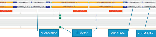
Figure 3.7 is a screenshot showing the amount of detail that is available on a timeline trace. This timeline shows three transform_reduce operations. The middle operation has been highlighted in gray to help separate the three annotated operations. The traces at the top show GPU activity and API calls; the bottom traces show activity on the system and related to the application on all the multiprocessor cores.
Parallel Nsight makes excellent use of color to help with interpretations, which is not shown in this grayscale image. A large monitor is suggested when using Parallel Nsight, as the timeline contains much information, including labels and scrollable, interactive regions.
Scaling Behavior of the CUDA API
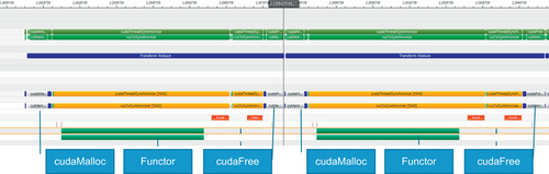
Looking at the timeline for the NLPCA example (Figure 3.8), we see that the functor occupies most of the GPU runtime. For three runs—using a full-size and a 10x and a 100x smaller data set—the timelines show that the repeated allocation and deallocation of a small scratch region of memory for the reduction consumes an ever greater percentage of the runtime. This consumption represents a scaling challenge in the current CUDA 4.0 implantation. The NVTX library was used to annotate the timeline.
Reducing the data by a factor of 10 times (Figure 3.9) shows that cudaMalloc() occupies more of the transform_reduce runtime.
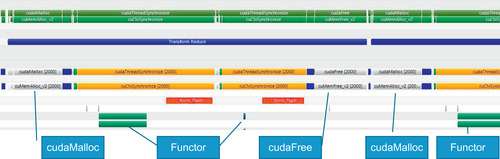
At 100 times smaller, when using 10,000 examples (Figure 3.10), the time to allocate and free temporary space for transform_reduce consumes a significant amount of the runtime.
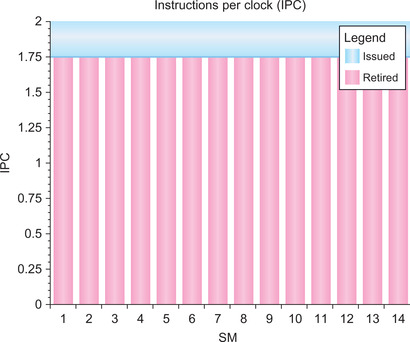
Even with the inefficiency of the allocation, Parallel Nsight graphically shows that the NLPCA functor achieves very high efficiency, as it performs nearly two operations per clock on all the multiprocessors of a C2050 (Figure 3.11).
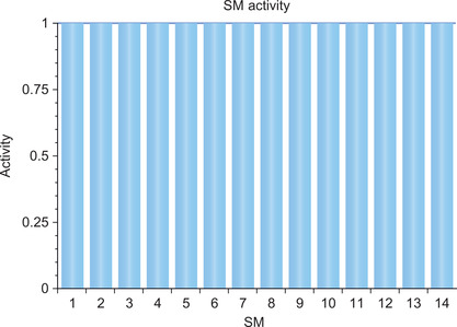
Parallel Nsight also reports that all the multiprocessors on the GPU are fully utilized (Figure 3.12), which rounds out the analysis that the CalcError functor is good use of the GPU capabilities.
Tuning and Analysis Utilities (TAU)
NIVIDA is not the only provider of analysis and debugging tools for CUDA. Tuning and Analysis Utilities (TAU) is a program and performance analysis tool framework being developed for the Department of Energy (DOE) Office of Sciences that is capable of gathering performance information through instrumentation of functions, methods, basic blocks, and statements. All C++ language features are supported, including templates and namespaces. TAU's profile visualization tool, paraprof, provides graphical displays of all the performance analysis results in aggregate and single node/context/thread forms. The user can quickly identify sources of performance bottlenecks in the application using the GUI. In addition, TAU can generate event traces that can be displayed with the Vampir, Paraver, or JumpShot trace visualization tools.
The paper “Parallel Performance Measurement of Heterogeneous Parallel Systems with GPUs” is the latest publication about the CUDA implementation (Malony et al., 2011; Malony, Biersdorff, Spear, & Mayanglamba, 2010). The software is available for free download from the Performance Research Laboratory (PRL). 2
Summary
With this accessible computational power, many past supercomputing techniques are now available for everyone to use—even on a laptop. In the 2006 paper “Reducing the Dimensionality of Data with Neural Networks,” Hinton and Salakhutdinov noted:
It has been obvious since the 1980s that backpropagation through deep autoencoders would be very effective for nonlinear dimensionality reduction, provided that computers were fast enough, data sets were big enough, and the initial weights were close enough to a good solution. All three conditions are now satisfied. (Hinton & Salakhutdinov, 2006, p. 506)
The techniques discussed in this chapter, including autoencoders, can be applied to a host of data fitting, data analysis, dimension reduction, vision, and classification problems. Conveniently, they are able to scale from laptops to the largest supercomputers in the world.
As this chapter showed, achieving high performance inside a functor does not guarantee good performance across all problem sizes. Sometimes the bottlenecks that limit performance are as subtle as the dynamic memory allocation of temporary space, as identified in the thrust::transform_reduce method.
Without being able to see what the GPU is doing, performance monitoring is guesswork. Having the right performance analysis tool is key to finding performance limitations. For this reason, the CUDA tool suite contains a number of common profiling and debugging tools that have been adapted to GPU computing. These are tools that Windows, UNIX, and Max developers are already comfortable with. Although each tool has both strengths and weaknesses, they all provide a useful view into GPU performance while requiring only a minimal learning investment. In this way, CUDA offers a smooth transition to massively parallel GPU programming.
..................Content has been hidden....................
You can't read the all page of ebook, please click here login for view all page.