
Chapter 10. CUDA in a Cloud and Cluster Environments
Distributed GPUs are powering the fastest supercomputers as CUDA scales to thousands of nodes using MPI, the de facto standard for distributed computing. NVIDIA's GPUDirect has accelerated the key operations in MPI, send (MPI_Send) and receive (MPI_Recv), for communication over the network instead of the PCIe bus. As the name implies, GPUDirect moves data between GPUs without involving the processor on any of the host systems. This chapter focuses on the use of MPI and GPUDirect so that CUDA programmers can incorporate these APIs to create applications for cloud computing and computational clusters. The performance benefits of distributed GPU computing are very real but dependent on the bandwidth and latency characteristics of the distributed communications infrastructure. For example, the Chinese Nebulae supercomputer can deliver a peak 2.98 PFlops (or 2,980 trillion floating point per second) to run some of the most computationally intensive applications ever attempted. Meanwhile, commodity GPU clusters and cloud computing provide turn-key resources for users and organizations. To run effectively in a distributed environment, CUDA developers must develop applications and use algorithms that can scale given the limitations of the communications network. In particular, network bandwidth and latency are of paramount importance.
Keywords
MPI, petaflop, data-mining, scalability, infiniband, gpuDirect, Kiviat, balance ratios, top 500
Distributed GPUs are powering the fastest supercomputers as CUDA scales to thousands of nodes using MPI, the de facto standard for distributed computing. NVIDIA's GPUDirect has accelerated the key operations in MPI, send (MPI_Send) and receive (MPI_Recv), for communication over the network instead of the PCIe bus. As the name implies, GPUDirect moves data between GPUs without involving the processor on any of the host systems. This chapter focuses on the use of MPI and GPUDirect so that CUDA programmers can incorporate these APIs to create applications for cloud computing and computational clusters. The performance benefits of distributed GPU computing are very real but dependent on the bandwidth and latency characteristics of the distributed communications infrastructure. For example, the Chinese Nebulae supercomputer can deliver a peak 2.98 PFlops (or 2,980 trillion floating point per second) to run some of the most computationally intensive applications ever attempted. Meanwhile, commodity GPU clusters and cloud computing provide turn-key resources for users and organizations. To run effectively in a distributed environment, CUDA developers must develop applications and use algorithms that can scale given the limitations of the communications network. In particular, network bandwidth and latency are of paramount importance.
At the end of this chapter, the reader will have a basic understanding of:
■ The Message Passing Interface (MPI).
■ NVIDIA's GPUDirect 2.0 technology.
■ How balance ratios act as an indicator of application performance on new platforms.
■ The importance of latency and bandwidth to distributed and cloud computing.
■ Strong scaling.
The Message Passing Interface (MPI)
MPI is a standard library based on the consensus of the MPI Forum (http://www.mpi-forum.org/), which has more than 40 participating organizations, including vendors, researchers, software library developers, and users. The goal of the forum is to establish a portable, efficient, and flexible standard that will be widely used in a variety of languages. Wide adoption has made MPI the “industry standard” even though it is not an IEEE (Institute of Electrical and Electronics Engineers) or ISO (International Organization for Standardization) standard. It is safe to assume that some version of MPI will be available on most distributed computing platforms regardless of vendor or operating system.
Reasons for using MPI:
■ Standardization: MPI is considered a standard. It is supported on virtually all HPC platforms.
■ Portability: MPI library calls will not need to be changed when running on platforms that support a version of MPI that is compliant with the standard.
■ Performance: Vendor implementations can exploit native hardware features to optimize performance. One example is the optimized data transport provided by GPUDirect.
■ Availability: A variety of implementations are available from both vendors and public domain software.
The MPI Programming Model
MPI is an API that was originally designed to support distributed computing for C and FORTRAN applications. It was first implemented in 1992, with the first standard appearing in 1994. Since then, language bindings and wrappers have been created for most application languages, including Perl, Python, Ruby, and Java. C bindings use the format MPI_Xxxx in which “Xxxx” specifies the operation. The methods MPI_Send() and MPI_Recv() are two examples that use this binding.
Just as with a CUDA execution configuration, MPI defines a parallel computing topology to connect groups of processes in an MPI session. It is important to note that with MPI the session size is fixed for the lifetime of the application. This differs from MapReduce (discussed later in this chapter), which is a popular framework for cloud computing that was designed for fault-tolerant distributed computing. All parallelism is explicit with MPI, which means that the programmer is responsible for correctly identifying parallelism and implementing parallel algorithms with the MPI constructs.
The MPI Communicator
A fundamental concept in MPI is the communicator, a distributed object that supports both collective and point-to-point communication. As the name implies, collective communications refers to those MPI functions involving all the processors within the defined communicator group. Point-to-point communications are used by individual MPI processes to send messages to each other.
By default, MPI creates the MPI_COMM_WORLD communicator immediately after the call to MPI_Init(). MPI_COMM_WORLD includes all the MPI processes in the application An MPI application can create multiple, separate communicators to separate messages associated with one set of tasks or group of processes from those associated with another. This chapter uses only the default communicator. Look to the many MPI books and tutorials on the Internet for more information about the use of communicator groups.
MPI Rank
Within a communicator, every process has its own unique, integer identifier assigned by the system when the process initializes. A rank is sometimes also called a “task ID.” Ranks are contiguous and begin at 0. They are often used in conditional operations to control execution of the MPI processes. A general paradigm in MPI applications is to use a master process, noted as rank 0, to control all other slave process of rank greater than 0.
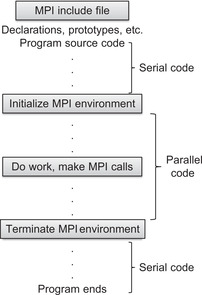
MPI programs are generally structured as shown in Figure 10.1.
Example 10.1, “A Basic MPI Program,” illustrates a C implementation of this framework by having each MPI process print out its rank:
#include "mpi.h"
#include <stdio.h>
int main(int argc, char *argv[])
{
int numtasks, rank, ret;
ret = MPI_Init(&argc,&argv);
if (ret != MPI_SUCCESS) {
printf ("Error in MPI_Init()!
");
MPI_Abort(MPI_COMM_WORLD, ret);
}
MPI_Comm_size(MPI_COMM_WORLD,&numtasks);
MPI_Comm_rank(MPI_COMM_WORLD,&rank);
printf ("Number of tasks= %d My rank= %d
", numtasks,rank);
/******* do some work *******/
MPI_Finalize();
}
MPI is usually installed and configured by the systems administrator. See the documentation for your cluster on how to compile and run this application.
NVIDIA, for example, makes the suggestion shown in Example 10.2, “NVIDIA Comment in the simpleMPI SDK Example,” to build their simpleMPI SDK example:
* simpleMPI.cpp: main program, compiled with mpicxx on linux/Mac platforms
*on Windows, please download the Microsoft HPC Pack SDK 2008
To build an application using CUDA and MPI in the same file, the nvcc command line in Example 10.3, “nvcc Command Line to Build basicMPI .cu,” works under Linux. The method links to the MPI library:
nvcc -I $MPI_INC_PATH basicMPI.cu -L $MPI_LIB_PATH –lmpich –o basicMPI
Usually mpiexec is used to start an MPI application. Some legacy implementations use mpirun. Example 10.4 shows the command and output when running the example with two MPI processes:
$ mpiexec -np 2 ./basicMPI
Number of tasks= 2 My rank= 1
Number of tasks= 2 My rank= 0
Master-Slave
A common design pattern in MPI programs is a master-slave paradigm. Usually the process that is designated as rank 0 is defined as the master. This process then directs the activities of all the other processes. The code snippet in Example 10.5, “A Master-Slave MPI Snippet,” illustrates how to structure master-slave MPI code:
MPI_Comm_size(MPI_COMM_WORLD,&numtasks);
MPI_Comm_rank(MPI_COMM_WORLD,&rank);
if( rank == 0){
// put master code here
} else {
// put slave code here
}
This chapter uses the master-slave programming pattern. MPI supports many other design patterns. Consult the Internet or one of the many MPI books for more information. A good reference is Using MPI (Gropp, Lusk, & Skjellum, 1999).
Point-to-Point Basics
MPI point-to-point communication sends messages between two different MPI processes. One process performs a send operation while the other performs a matching read. MPI guarantees that every message will arrive intact without errors. Care must be exercised when using MPI, as deadlock will occur when the send and receive operations do not match. Deadlock means that neither the sending nor receiving process can proceed until the other completes its action, which will never happen when the send and receive operations do not match. CUDA avoids deadlock by sharing data between the threads of a thread block with shared memory. This frees the CUDA programmer from having to explicitly match read and write operations but still requires the programmer to ensure that data is updated appropriately.
MPI_Send() and MPI_Recv() are commonly used blocking methods for sending messages between two MPI processes. Blocking means that the sending process will wait until the complete message has been correctly sent and the receiving process will block while waiting to correctly receive the complete message. More complex communications methods can be built upon these two methods.
Message size is determined by the count of an MPI data type and the type of the data. For portability, MPI defines the elementary data types. Table 10.1 lists data types required by the standard.
How MPI Communicates
MPI can use optimized data paths to send and receive messages depending on the network communications hardware. For example, MPI applications running within a computational node can communicate via fast shared memory rather than send data over a physical network interface card (NIC). Minimizing data movement is an overarching goal for MPI vendors and those who develop the libraries because moving data simply wastes precious time and degrades MPI performance.
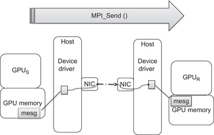
In collaboration with vendors and software organizations, NVIDIA created GPUDirect to accelerate MPI for GPU computing. The idea is very simple: take the GPU data at the pointer passed to MPI_Send() and move it to the memory at the pointer to GPU memory used in the MPI_Recv() call. Don't perform any other data movements or rely on other processors. This process is illustrated in Figure 10.2. Although simple in concept, implementation requires collaboration between vendors, drivers, operating systems, and hardware.
InfiniBand (IB) is a commonly used high-speed, low-latency communications link in HPC. It is designed to be scalable and is used in many of the largest supercomputers in the world. Most small computational clusters also use InfiniBand for price and performance reasons. Mellanox is a well-known and respected vendor of InfiniBand products.
NVIDIA lists the following changes in the Linux kernel, the NVIDIA Linux CUDA driver, and the Mellanox InfiniBand driver:
■ Linux kernel modifications:
■ Support for sharing pinned pages between different drivers.
■ The Linux Kernel Memory Manager (MM) allows NVIDIA and Mellanox drivers to share the host memory and provides direct access for the latter to the buffers allocated by the NVIDIA CUDA library, thus providing Zero Copy of data and better performance.
■ NVIDIA driver:
■ Allocated buffers by the CUDA library are managed by the NVIDIA driver.
■ We have added the modifications to mark these pages to be shared so the Kernel MM will allow the Mellanox InfiniBand drivers to access them and use them for transportation without the need for copying or repinning them.
■ Mellanox OFED1 drivers:
■ We have modified the Mellanox InfiniBand driver to query memory and to be able to share it with the NVIDIA Tesla drivers using the new Linux Kernel MM API.
■ In addition, the Mellanox driver registers special callbacks to allow other drivers sharing the memory to notify any changes performed during runtime in the shared buffers state in order for the Mellanox driver to use the memory accordingly and to avoid invalid access to any shared pinned buffers.
The result is the direct data transfer path between the send and receive buffers that provides a 30 percent increase in MPI performance.
Figure 10.2 shows that a registered region of memory can be directly transferred to a buffer in the device driver. Both the NIC and the device driver on the sending host know about this buffer, which lets the NIC send the data over the network interconnect without any host processor intervention. Similarly, the device driver and NIC on the receiving host know about a common receive buffer. When the GPU driver is notified that the data has arrived intact, it is transferred to the receiving GPU (GPUR in Figure 10.2).
There are two ways for a CUDA developer to allocate memory in this model:
■ Use cudaHostRegister().
■ With the 4.0 driver, just set the environmental variable CUDA_NIC_INTEROP=1. This will tell the driver to use an alternate path for cudaMallocHost() that is compatible with the IB drivers. There is no need to use cudaHostRegister().
Bandwidth
Network bandwidth is a challenge in running distributed computations. The bandwidths listed in Table 10.2 show that most network interconnects transfer data significantly slower than the PCIe bus. (QDR stands for Quad Data Rate InfiniBand. DDR and SDR stand for double and single data rate, respectively.)
A poor InfiniBand network can introduce an order of magnitude slowdown relative to PCIe speeds, which emphasizes the first of the three rules of efficient GPU programming introduced in Chapter 1: “Get the data on the GPGPU and keep it there.” It also raises portability issues for those who wish to ship distributed MPI applications. Unfortunately, users tend to blame the application first for poor performance rather than the hardware.
Balance Ratios
Deciding whether an application or algorithm will run effectively across a network is a challenge. Of course, the most accurate approach is to port the code and benchmark it. This may be impossible due to lack of funding and time. It may also result in a lot of needless work.
Balance ratios are a commonsense approach that can provide a reasonable estimation about application or algorithm performance that does not require first porting the application. These metrics are also used to evaluate hardware systems as part of a procurement process (Farber, 2007).
Balance ratios define a system balance that is quantifiable and—with the right choice of benchmarks—provides some assurance that an existing application will run well on a new computer. The challenge lies in deciding what characteristics need to be measured to determine whether an application will run well on a GPU or network of GPUs.
Most GPU applications are numerically intensive, which suggests that all GPU-based metrics should be tied to floating-point performance. Comparisons can then be made between systems and cards with different floating-point capabilities. Bandwidth limitations are an important metric to tie to numerical performance, as global memory, the PCIe bus, and network connectivity are known to bottleneck GPU performance for most applications. As shown in Equation 10.1 the ratios between floating-point performance and the bandwidths available to keep the floating-point processors busy can be calculated from vendor and hardware information. This ratio makes it easy to see that a hardware configuration that moves data over a four-times DDR InfiniBand connection can cause an order of magnitude decrease in application performance versus the same application running on hardware that moves data across the PCIe bus.
(10.1)
These observations are not new in HPC. The January 2003 Report of the National Science Foundation Blue-Ribbon Advisory Panel on Cyberinfrastructure, 2 known as the Atkins Report, specifies some desirable metrics that are tied to floating-point performance:
■ At least 1 byte of memory per flop/s.
■ Memory bandwidth (byte/s/flop/s) ≥ 1.
■ Internal network aggregate link bandwidth (bytes/s/flop/s) ≥ 0.2.
■ Internal network bi-section bandwidth (bytes/s/flop/s) ≥ 0.1.
■ System sustained productive disk I/O bandwidth (byte/s/flop/s) ≥ 0.001.
Keep in mind that numerical values presented in the Atkins Report are for desirable ratios based on their definition of a “representative” workload. Your application may have dramatically different needs. For this reason, it is worthwhile to evaluate your applications to see what ratios currently work and what ratios need to be improved.
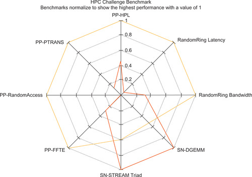
A good approach is to use benchmarks to evaluate system performance. This is the thought behind the Top 500 list that is used to rank the fastest supercomputers in the world. The HPC Challenge (HPCC) website3 provides a more extensive test suite. It will also generate a Kiviat diagram (Kiviat diagrams are similar to the radar plots in Microsoft Excel) to compare systems based on the standard HPCC benchmarks. A well-balanced system looks symmetrical on these plots because it performs well on all tests. High-performance balanced systems visually stand out because they occupy the outermost rings. Out-of-balance systems are distorted, as can be seen in Figure 10.3.
The HPCC website is a good source for benchmarks and comparative data on different computational systems. Be aware that synthetic benchmarks such as those on the HPCC website are very good at stressing certain aspects of machine performance, but they do represent a narrow view into machine performance.
To provide a more realistic estimate, most organizations utilize benchmark evaluation suites that include some sample production codes to complement synthetic benchmarks—just to see if there is any unexpected performance change, either good or bad. Such benchmarks can also provide valuable insight into how well the processor and system components work together on real-world applications; plus, they can uncover issues that can adversely affect performance such as immature compilers and/or software drivers.
The key point behind balance ratios is that they can help the application programmer or system designer decide whether some aspect of a new hardware system will bottleneck an application. Although floating-point performance is important, other metrics such as memory capacity, storage bandwidth, and storage capacity might be a gating factor. The memory capacity of current GPUs, for example, can preclude the use of some applications or algorithms.
Considerations for Large MPI Runs
In designing distributed applications, it is important to consider the scalability of all aspects of the application—not just of the computation!
Many legacy MPI applications were designed at a time when an MPI run that used from 10 to 100 processing cores was considered a “large” run. (Such applications might be good candidates to port to CUDA so that they can run on a single GPU.) A common shortcut taken in these legacy applications is to have the master process read data from a file and distribute it to the clients according to some partitioning scheme. This type of data load cannot scale, as the master node simply cannot transfer all the data for potentially tens of thousands of other processes. Even with modern hardware, the master process will become a bottleneck, which can cause the data load to take longer than the actual calculation.
Scalability of the Initial Data Load
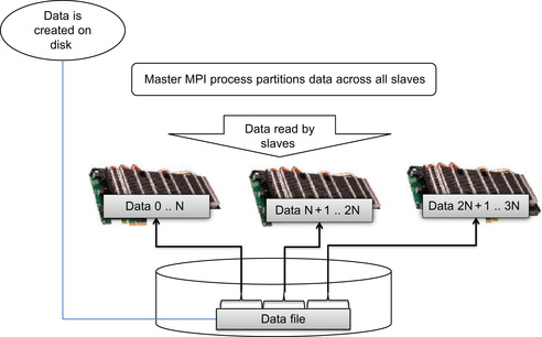
A better approach is to have each process read its own data from a file on a distributed file system. Each process is provided with the filename of a data file that contains the data. They then open the file and perform whatever seek and other I/O operations are needed to access and load the data. All the clients then close the file to free system resources. This simple technique can load hundreds of gigabytes of data into large supercomputers very quickly. The process is illustrated in Figure 10.4.
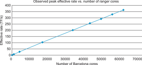
With this I/O model, much depends on the bandwidth capabilities of the file system that holds the data. Modern parallel distributed file systems can deliver hundreds of gigabytes per second of storage bandwidth when concurrently accessed by multiple processes. The freely available Lustre file system4 can deliver hundreds of gigabytes per second of file system bandwidth using this technique and demonstrated scaling to 60,000 MPI processes as shown in Figure 10.5. Commercial file systems such as GPFS (General Parallel File System) by IBM and PanFS by Panasas also scale to hundreds of gigabytes per second and tens of thousands of MPI processes. To achieve high performance, these file systems need to be accessed by a number of concurrent distributed processes. It is not recommended to use this technique with large numbers of MPI clients on older NFS and CIFS file systems.
Using MPI to Perform a Calculation
The general mapping introduced in Chapter 2 has been used in an MPI distributed environment to scale to 500 GPUs on the TACC Longhorn supercomputer. The same mapping has been used to scale to more than 60,000 processing cores on both the CM-200 Connection Machine (Farber, 1992) and the TACC Ranger Supercomputer (Farber & Trease, 2008).
During these runs, the rank 0 process was designated as the master process in a conventional master-slave configuration. The master then:
■ Initiated the data load as described previously. Even when using hundreds of gigabytes of data, the data load took only a few seconds using a modern parallel distributed file system.
■ Performed other initializations.
■ Runs the optimization procedure and directs the slave processes.
■ To make the best use of the available resources, the master node also evaluates the objective function along with the slave processes.
■ Most production runs used a variant of Powell's method, as described in Numerical Recipes (Press, Teukolsky, & Vetterling, 2007a) or Conjugant Gradient (also described in Numerical Recipies).
■ On each evaluation of the objective function:
■ Uses MPI_Bcast() to broadcast the parameters to all the slave processes.
■ Performs its own local calculation of the objective function.
■ Calls MPI_Reduce() to retrieve the total sum of all partial results.
■ In general, the MPI_Reduce() operation is highly optimized and scales according to O(log2(ntasks)), where ntasks is the number reported by MPI_Comm_size().
■ Supplies the result of the objective function to the optimization method, which causes either:
■ Another evaluation of the objective function.
■ Completion of the optimization process.
The slave processes (those processes with a rank greater than 0):
■ Initiate the data load as described previously.
■ Remain in an infinite loop until told it is time to exit the application by the master. Inside the loop, each slave:
■ Reads the parameters from the master node.
■ Calculates the partial sum of the objective function.
■ Sends the partial results to the master when requested.
Check Scalability
The scaling behavior of a distributed application is a key performance metric. Applications that exhibit strong scaling run faster as the number of processors are added to a fixed problem size. Linear scaling is a goal for distributed applications because the runtime of an application scales linearly with the amount of computational available (e.g., a two-times larger system will run the problem in half the time, a four-times larger system will run the problem in one-fourth the time, etc.). Embarrassingly parallel problems can exhibit linear runtime behavior because each computation is independent of each other. Applications that require communication to satisfy some dependency can generally achieve at best near-linear scaling. For example, an O(log2(N)) reduction operation will cause the scaling behavior to slowly diverge from a linear speedup according to processor count. Figure 10.5 illustrates near-linear scaling to 60,000 processing cores using the PCA objective function discussed in Chapter 3.
The 386 teraflop per second effective rate for the AMD Barcelona based TACC Ranger supercomputer reported in Figure 10.5 includes all communications overhead. A 500 GPU-based supercomputer run could deliver nearly 500 teraflops of single-precision performance. A colleague refers to these as “honest flops,” as they reflect the performance a real production run would deliver.
The effective rate is defined for the PCA mapping is shown in Equation 10.2, “Definition of effective rate for the PCA parallel mapping”:
(10.2)
■ TotalOpCount is the number of floating-point operations performed in a call to an objective function.
■ Tbroadcast is the time required to broadcast the parameters to all the slave processes.
■ Tobjectfunc is the time consumed in calculating the partial results across all the clients. This is generally the time taken by the slowest client.
■ Treduce is the time required by the reduction of the partial results.
Cloud Computing
Cloud computing is an infrastructure paradigm that moves computation to the Web in the form of a web-based service. The idea is simplicity itself: institutions contract with Internet vendors for computational resources instead of providing those resources themselves through the purchase and maintenance of computational clusters and supercomputer hardware. As expected with any computational platform—especially one utilized for high performance and scientific computing—performance limitations within the platform define which computational problems will run well.
Unlike MPI frameworks, cloud computing requires that application be tolerant of both failures and high latency in point-to-point communications. Still, MPI is such a prevalent API that most cloud computing services provide and support it. Be aware that bandwidth and latency issues may cause poor performance when running MPI on a cloud computing infrastructure.
MPI utilizes a fixed number of processes that participate in the distributed application. This number is defined at application startup—generally with mpiexec. In MPI, the failure of any one process in a communicator affects all processes in the communicator, even those that are not in direct communication with the failed process. This factor contributes to the lack of fault tolerance in MPI applications.
MapReduce is a fault-tolerant framework for distributed computing that has become very popular and is widely used (Dean & Ghemawat, 2010). In other words, the failure of a client has no significant effect on the server. Instead, the server can continue to service other clients. What makes the MapReduce structure robust is that all communication occurs in a two-party context where one party (e.g., process) can easily recognize that the other party has failed and can decide to stop communicating with it. Moreover, each party can easily keep track of the state held by the other party, which facilitates failover.
A challenge with cloud computing is that many service providers use virtual machines that run on busy internal networks. As a result, communications time can increase. In particular, the time Treduce is very latency-dependent, as can be seen in Equation 10.2. For tightly coupled applications (e.g., applications with frequent communication between processes), it is highly recommended that dedicated clusters be utilized. In particular, reduction operations will be rate-limited by the slowest process in the group. That said, papers like “Multi-GPU MapReduce on GPU Clusters” (Stuart & Owens, 2011) demonstrate that MapReduce is an active area of research.
A Code Example
The objective function from the nlpcaNM.cu example from Chapter 3 was adapted to use MPI and this data load technique.
Data Generation
A simple data generator was created that uses the genData() method from nlpcaNM.cu. This program simply writes a number of examples to a file. Both the filename and number of examples are specified on the command line. The complete source listing is given in Example 10.6, “Source for genData.cu”:
#include <iostream>
#include <fstream>
#include <stdlib.h>
using namespace std;
// get a uniform random number between -1 and 1
inline float f_rand() {
return 2*(rand()/((float)RAND_MAX)) -1.;
}
template <typename Real>
void genData(ofstream &outFile, int nVec, Real xVar)
{
Real xMax = 1.1; Real xMin = -xMax;
Real xRange = (xMax - xMin);
for(int i=0; i < nVec; i++) {
Real t = xRange * f_rand();
Real z1 = t + xVar * f_rand();
Real z2 = t*t*t + xVar * f_rand();
outFile.write((char*) &z1, sizeof(Real));
outFile.write((char*) &z2, sizeof(Real));
}
}
int main(int argc, char *argv[])
{
if(argc < 3) {
fprintf(stderr,"Use: filename nVec
");
exit(1);
}
ofstream outFile (argv[1], ios::out | ios::binary);
int nVec = atoi(argv[2]);
#ifdef USE_DBL
genData<double>(outFile, nVec, 0.1);
#else
genData<float>(outFile, nVec, 0.1);
#endif
outFile.close();
return 0;
}
The program can be saved in a file and compiled as shown in Example 10.7, “Building genData.cu.” The C preprocessor variable USE_DBL specifies whether the data will be written as 32-bit or 64-bit binary floating-point numbers:
nvcc -D USE_DBL genData.cu -o bin/genData64
nvcc genData.cu -o bin/genData32
Data sets can be written via the command line. For example, Example 10.8, “Creating a 32-Bit File with genData.cu,” writes 10M 32-bit floats to a file nlpca32.dat.
bin/genData32 nlpca32.dat 10000000
It is very easy to specify the wrong file during runtime. This simple example does not provide version, size, or any other information useful for sanity checking. The Google ProtoBufs project is recommend for a production quality file and streaming data format. 5 Google uses this project for almost all of its internal RPC protocols and file formats.
The nlpcaNM.cu example code from Chapter 3 was modified to run in an MPI environment. The changes are fairly minimal but are distributed throughout the code. Only code snippets are provided in the following discussion. The entire code can be downloaded from the book website. 6
The variable nGPUperNode was defined at the beginning of the file. It is assumed that the number of MPI processes per node will equal the number of GPUs in each node (meaning one MPI process is per GPU). The value of nGPUperNode allows each MPI process to call cudaSetDevice() correctly to use different devices. Other topologies are possible including using one MPI process per node for all GPUs. See Example 10.9, “Modification of the Top of nlpcaNM.cu to Use Multiple GPUs per Node”:
#include "mpi.h"
const static int nGPUperNode=2;
}
The main() method of nlpcaNM.cu has been modified with the MPI framework shown in Figure 10.1 using the code shown in Example 10.1 (see Example 10.10, “Modified main() method for nlpcaNM.cu”:
#include <stdio.h>
int main(int argc, char *argv[])
{
int numtasks, rank, ret;
if(argc < 2) {
fprintf(stderr,"Use: filename
");
exit(1);
}
ret = MPI_Init(&argc,&argv);
if (ret != MPI_SUCCESS) {
printf ("Error in MPI_Init()!
");
MPI_Abort(MPI_COMM_WORLD, ret);
}
MPI_Comm_size(MPI_COMM_WORLD,&numtasks);
MPI_Comm_rank(MPI_COMM_WORLD,&rank);
printf ("Number of tasks= %d My rank= %d
", numtasks,rank);
/******* do some work *******/
#ifdef USE_DBL
trainTest<double> ( argv[1], rank, numtasks );
#else
trainTest<float> ( argv[1], rank, numtasks);
#endif
MPI_Finalize();
return 0;
}
The setExamples() method was modified to allocate memory on different GPUs. See Example 10.11, “Modified setExamples Method for nlpcaNM.cu”:
void setExamples(thrust::host_vector<Real>& _h_data) {
nExamples = _h_data.size()/exLen;
// copy data to the device
int rank;
MPI_Comm_rank(MPI_COMM_WORLD,&rank);
cudaSetDevice(rank%nGPUperNode);
d_data = thrust::device_vector<Real>(nExamples*exLen);
thrust::copy(_h_data.begin(), _h_data.end(), d_data.begin());
d_param = thrust::device_vector<Real>(nParam);
}
Example 10.12, “Modified trainTest Method for nlpcaNM.cu,” shows how the data is loaded from disk:
#include <fstream>
template <typename Real>
void trainTest(char* filename, int rank, int numtasks)
{
ObjFunc<Real> testObj;
const int nParam = testObj.nParam;
cout << "nParam " << nParam << endl;
// read the test data
ifstream inFile (filename, ios::in | ios::binary);
// position 0 bytes from end
inFile.seekg(0, ios::end);
// determine the file size in bytes
ios::pos_type size = inFile.tellg();
// allocate number of Real values for this task
//(assumes a multiple of numtasks)
int nExamplesPerGPU = (size/(sizeof(Real)*testObj.exLen))/numtasks;
thrust::host_vector<Real> h_data(nExamplesPerGPU*testObj.exLen);
// seek to the byte location in the file
inFile.seekg(rank*h_data.size()*sizeof(Real), ios::beg);// allocate number of Real values for this task
inFile.seekg(rank*h_data.size()*sizeof(Real));
// read bytes from the file into h_data
inFile.read((char*)&h_data[0], h_data.size()*sizeof(Real));
// close the file
inFile.close();
testObj.setExamples(h_data);
int nExamples = testObj.get_nExamples();
if(rank > 0) {
testObj.objFunc( NULL );
return;
}
...Nelder-Mead code goes here
int op=0; // shut down slave processes
MPI_Bcast(&op, 1, MPI_INT, 0, MPI_COMM_WORLD);
}
In this example, binary input stream, infile is opened to read the data in the file filename. After that:
■ The size of the file is determined.
■ Each of the numtasks processes is assigned an equal amount of the data based on the file size and the number of data per example. The logic is simplified by assuming that the number of examples is a multiple of numtasks.
■ The host vector h_data is allocated.
■ A seek operation moves to the appropriate position in the file.
■ The data is read into h_data and handed off to setExamples() to be loaded onto the device.
■ As shown in Figure 10.6, the rank of the process is tested:
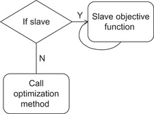
■ If the rank is greater than zero, this process is a slave. The objective function is called with a NULL parameters argument and the training finishes when that method exits.
■ If the process is a master, the Nelder-Mead optimization code is called.
The objective function implements the logic for both the master and slave processes, as illustrated in Figure 10.7.
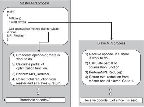
The objective function (Example 10.13) belongs to a slave process when the MPI rank is greater than 0. In this case, the slave state machine:
1. Allocates space in pinned memory for the parameters.
2. It waits for an operation code to be broadcast from the master.
a. The master tells the slave that all work is done with a zero op code and that it should return.
b. Otherwise, the slave will move to the next step.
3. The slave waits for the host to broadcast the parameters.
4. After the master broadcasts the parameters, the slave runs the objective function on its data and blocks waiting for the master to ask for the result.
5. After the master requests the reduction result the slave returns to wait for an op code in step 2. This process continues until the master sends a 0 op code.
The objective function (Example 10.13) belongs to the master process when the rank is 0. In this case, the master:
1. Broadcasts a nonzero op code to let all the slaves know there is work to do.
2. Broadcasts the parameters to all the slaves.
3. Runs the objective function on its data.
4. Performs a reduction to sum the partial values from the slave processes.
5. Returns to continue running the optimization method.
Real objFunc(Real *p)
{
int rank,op;
Real sum=0.;
MPI_Comm_rank(MPI_COMM_WORLD,&rank);
cudaSetDevice(rank%nGPUperNode);
if(nExamples == 0) {
cerr << "data not set " << endl; exit(1);
}
CalcError getError(thrust::raw_pointer_cast(&d_data[0]),
thrust::raw_pointer_cast(&d_param[0]),
nInput, exLen);
if(rank > 0) { // slave objective function
Real *param;
cudaHostAlloc(¶m, sizeof(Real)*nParam,cudaHostAllocPortable);
for(;;) { // loop until the master says I am done.
MPI_Bcast(&op, 1, MPI_INT, 0, MPI_COMM_WORLD);
if(op==0) {
cudaFreeHost(param);
return(0);
}
if(sizeof(Real) == sizeof(float))
MPI_Bcast(¶m[0], nParam, MPI_FLOAT, 0, MPI_COMM_WORLD);
else
MPI_Bcast(¶m[0], nParam, MPI_DOUBLE, 0, MPI_COMM_WORLD);
thrust::copy(param, param+nParam, d_param.begin());
Real mySum = thrust::transform_reduce(
thrust::counting_iterator<unsigned int>(0),
thrust::counting_iterator<unsigned int> (nExamples),
getError,
(Real) 0.,
thrust::plus<Real>());
if(sizeof(Real) == sizeof(float))
MPI_Reduce(&mySum, &sum, 1, MPI_FLOAT, MPI_SUM, 0, MPI_COMM_WORLD);
else
MPI_Reduce(&mySum, &sum, 1, MPI_DOUBLE, MPI_SUM, 0, MPI_COMM_WORLD);
}
} else { // master process
double startTime=omp_get_wtime();
op=1;
MPI_Bcast(&op, 1, MPI_INT, 0, MPI_COMM_WORLD);
if(sizeof(Real) == sizeof(float))
MPI_Bcast(&p[0], nParam, MPI_FLOAT, 0, MPI_COMM_WORLD);
else
MPI_Bcast(&p[0], nParam, MPI_DOUBLE, 0, MPI_COMM_WORLD);
thrust::copy(p, p+nParam, d_param.begin());
Real mySum = thrust::transform_reduce(
thrust::counting_iterator<unsigned int>(0),
thrust::counting_iterator<unsigned int>(nExamples),
getError,
(Real) 0.,
thrust::plus<Real>());
if(sizeof(Real) == sizeof(float))
MPI_Reduce(&mySum, &sum, 1, MPI_FLOAT, MPI_SUM, 0, MPI_COMM_WORLD);
else
MPI_Reduce(&mySum, &sum, 1, MPI_DOUBLE, MPI_SUM, 0, MPI_COMM_WORLD);
objFuncCallTime += (omp_get_wtime() - startTime);
objFuncCallCount++;
}
return(sum);
}
The application completes after the optimization method returns in the master process. The final line in testTrain() broadcasts a zero opcode to all the slaves to tell them to exit. The master process then returns to main() to shut down MPI normally.
Table 10.3 shows that running the MPI version of nlpcaNM.cu on two GPUs provides a nearly double increase in performance. No network was used as both GPUs were inside the same system. The example code from this chapter ran unchanged to deliver near-linear scalability to 500 GPUs on the Texas Advanced Computing Center (TACC) Longhorn supercomputer cluster. Many thanks to TACC for providing access to this machine. 8
| Number of GPUs | Time per Objective Function | Speedup over one GPU |
|---|---|---|
| 1 | 0.0102073 | |
| 2 | 0.00516948 | 1.98 |
Summary
MPI and GPUDirect give CUDA programmers the ability to run high-performance applications that far exceed the capabilities of a single GPU or collection of GPUs inside a single system. Scalability and performance within a node are key metrics to evaluate distributed applications. Those applications that exhibit linear or near-linear scalability have the ability to run on the largest current and future machines. For example, the parallel mapping discussed in this chapter, plus Chapter 2 and Chapter 3, is now nearly 30 years old. At the time it was designed, a teraflop of computing power was decades beyond the reach of even the largest government research organizations. Today, it runs very effectively on GPU devices, clusters, and even the latest supercomputers. It will be interesting to see how many yottaFlops (1024 flops) will be available 30 years from now. Meanwhile, this mapping provides a scalable solution for large data-mining and optimization tasks.
..................Content has been hidden....................
You can't read the all page of ebook, please click here login for view all page.