
Chapter 6. Efficiently Using GPU Memory
The importance of efficiently using GPU memory cannot be overstated. With roughly three-orders-of-magnitude difference in speed between the fastest on-chip register memory and mapped data that must traverse the PCIe bus, literate CUDA developers must understand the most efficient ways to use memory. Latency hiding through ILP or TLP is essential to application performance. Prefetching can keep more memory transactions in flight to move data to fast memory and speed even memory bandwidth-limited reduction operations. Irregular data structures are a challenge with current GPU technology, but some techniques can preserve performance even with random memory accesses. However, finding more and better ways to utilize GPU memory is an area of active research as new libraries become available that support irregular data structures such as graphs and sparse matrices.
Keywords
Prefetch, reduction, L2 cache, L1 cache, PTX, mapped memory, profiling
The importance of efficiently using GPU memory cannot be overstated. With roughly three-orders-of-magnitude difference in speed between the fastest on-chip register memory and mapped host memory that must traverse the PCIe bus, literate CUDA developers must understand the most efficient ways to use memory. Latency hiding through ILP or TLP is essential to application performance. Prefetching can keep more memory transactions in flight to move data to fast memory and speed even memory bandwidth-limited reduction operations. Irregular data structures are a challenge with current GPU technology, but some techniques can preserve performance even with random memory accesses. However, finding more and better ways to utilize GPU memory is an area of active research as new libraries become available that support irregular data structures such as graphs and sparse matrices.
At the end of this chapter, the reader will have a basic understanding of:
■ Using prefetch to better utilize global memory.
■ Efficient use of registers, shared, and global memory in an ILP-based reduction kernel.
■ How to write generic methods that utilize functors.
■ Techniques to speed problems that have irregular and random memory accesses.
■ Generic approaches and libraries for sparse matrices.
■ Graph centrality metrics and codes that can provide 10- to 50-times speedups.
■ Performance reasons to use SoA.
■ Stencils and tiles.
Reduction
Reduction operations perform common tasks such as finding the minimum, maximum, or sum of a vector. Writing a high-performance reduction for GPU computing is surprisingly complex because it requires a detailed understanding of CUDA memory spaces and the execution model.
The thrust API provides a simple interface that hides all the complexity of a reduction, making it both flexible and easy to use. Thrust uses a reduction designed by Mark Harris at NVIDIA. The paper and example code demonstrating various optimizations for reduction are included with the NVIDIA SDK in the reduction directory. Both the paper and code are recommended reading.
This chapter provides a reduction example that ties together much of the discussion in previous chapters and extends the reduction created by Mark Harris:
■ C++ templates extend the generality of the reduction code to use user-defined types such as floats, doubles, integers, long integers, and others.
■ New features of compute 2.0 devices such as the PTX prefetch instruction and inline assembly code are used to increase global memory read performance.
■ Temporary storage is passed to the reduction method so that the programmer can eliminate redundant cudaMalloc() and cudaFree() operations that slow the thrust implementation as noted in Chapter 3.
■ The passing and use of inline functors is demonstrated to create a generic reduction operation that is applicable more than just finding the sum of a vector.
The Reduction Template
The following walkthrough of the code for the generic reduction template functionReduce.h covers the key concepts and thinking behind each section of code. The code snippets can be combined to construct the complete functionReduce.h source file.
The #ifndef check of the preprocessor variable REDUCE_H protects against compiler errors, should the template file ever be included multiple times; see Example 6.1, “Part 1 of functionReduce.h”:
#ifndef REDUCE_H
#define REDUCE_H
For simplicity, the following section of the template defines the number of blocks and threads for use on a C2050 or C2070 GPU. These definitions can be set manually from the information determined by the NVIDIA SDK code deviceQuery. A production version of this template might query the device properties and set these values automatically, as in Example 6.2, “Part 2 of functionReduce.h”:
// Define the number of blocks as a multiple of the number of SM
// and the number of threads as the maximum resident on the SM
#define N_BLOCKS (1*14)
#define N_THREADS 1024
#define WARP_SIZE 32
Example 6.3 starts the definition of the _functionReduce() method:
template <class T, typename UnaryFunction, typename BinaryFunction>
__global__ void
_functionReduce(T *g_odata, unsigned int n, T initVal, UnaryFunction fcn, BinaryFunction fcn1)
{
Notice that:
■ All variables are defined in terms of the template variable type T for generality. For example, T can be defined as a float, double, int, or char type.
■ A scratch region of memory is provided so that each SM can write a single partial result of type T to global memory. Passing a pointer allows reuse of the scratch space to avoid the repetitive allocate and free overhead observed in the thrust reduction operation in Chapter 3.
■ The number of calls to the unary function fcn() is passed to via the variable n.
■ The unary function fcn() can be defined to fetch data from memory or calculate some result on the fly. For example, the test code that follows this template defines fcn() as a functor that fetches data from a vector in global memory. Alternative functors can fetch data from complex data structures in global memory, calculate a result based on numerous data structures in memory, perform a table lookup, or avoid the use of global memory entirely by returning some constant or computed value.
■ As with the thrust reduction call, an initial value is passed. This can be the starting value for a sum, or an initial value to use in a minimum() or maximum() reduction.
■ The binary function fcn1() defines a generic operation on two of the values returned by fcn(). Examples include the thrust::plus() functor when a sum is desired. Similarly, the thrust::minimum() or thrust::maximum() functors can be used. Alternatively, the user can provide his or her own binary functor.
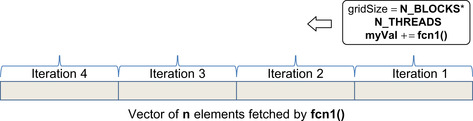
Each thread on the GPU starts out with the register variable myVal set to initVal. Then each thread iterates through and calculates a partial result in fast register memory. If fcn1() were a plus() operation and fcn() fetched data from a vector in global memory, then myVal would contain the partial sums of all the vector elements as shown in Figure 6.1. This step reduces the data from n values (which could be on the order of millions) to N_BLOCKS*N_THREADS partial values. Note that the loop traverses the vector in reverse order, starting at the end and working toward the beginning. This approach gives the author of fcn() the opportunity to confirm that any prefetching does not access data prior to the start of the vector. Thus fcn() does not need to know the end or length of the vector, which saves memory and a register. See Example 6.4, “Part 4 of functionReduce.h”:
T myVal = initVal;
{ // 1) Use fastest memory first.
const int gridSize = blockDim.x*gridDim.x;
for(int i = n-1 -(blockIdx.x * blockDim.x + threadIdx.x);
i >= 0; i -= gridSize)
myVal = fcn1(fcn(i), myVal);
}
After this loop completes, the register variable myVal contains N_BLOCKS*N_THREADS partial values. In CUDA, register variables are not accessible to other threads. For this reason, it is necessary to move the partial values stored in myVal to slower shared memory so that they can be accessed by other threads. The transfer from register to shared memory happens in step 2 shown in Example 6.5. This is a parallel transfer all the threads in each thread block to the shared memory variable smem inside each SM.
Shared memory is a valuable resource, so only the minimum amount is allocated. Based on the discussion of ILP in Chapter 4, the parallelism of only one warp of threads is used to perform the reduction from N_THREADS partial values on each SM to WARP_SIZE partial values. The register variable myVal already contains the correct values for the first warp. Thus, the shared memory smem variable needs only contain the contents of the myVal register variables in threads with a threadIdx.x greater than or equal to WARP_SIZE. As a result, smem can be allocated to contain WARP_SIZE fewer elements than N_THREADS.
Because the transfer from register to shared memory occurs in parallel, the CUDA __syncthreads() method must be called after the assignment to ensure that all the elements of smem have been written. All of this happens in the few lines of Example 6.5, “Part 5 of functionReduce.h”:
// 2) Use the second fastest memory (shared memory) in a warp
// synchronous fashion.
// Create shared memory for per-block reduction.
// Reuse the registers in the first warp.
volatile __shared__ T smem[N_THREADS-WARP_SIZE];
// put all the register values into a shared memory
if(threadIdx.x >= WARP_SIZE) smem[threadIdx.x - WARP_SIZE] = myVal;
__syncthreads(); // wait for all threads in the block to complete.
At this point in the kernel, there is no reason to use more than the number of threads in one warp because the SM can issue only a single instruction per warp. Because there are no unresolved data dependencies, a single warp is sufficient to keep the SM busy in reducing the contents of shared memory from (N_THREADS – WARP_SIZE) elements to WARP_SIZE partial values on each SM. 1 That is why a conditional is used to keep only threads with a threadIdx.x less than WARP_SIZE active. See Example 6.6, “Part 6 of functionReduce.h”:
if(threadIdx.x < WARP_SIZE) {
// now using just one warp. The SM can only run one warp at a time
#pragma unroll
for(int i=threadIdx.x; i < (N_THREADS − WARP_SIZE); i += WARP_SIZE)
myVal = fcn1(myVal,(T)smem[i]);
smem[threadIdx.x] = myVal; // save myVal in this warp to the start of smem
}
What remains is to reduce the values in one warp to a single value on each SM. This equates to N_BLOCKS partial values, as N_BLOCKS was defined to use one block per SM. It is worth noting that the parallelism within the warp at this point does not contribute much to the performance, as only five calls to fcn1() are made in Example 6.7.
An alternative implementation can use a simple loop over WARP_SIZE running on a single thread (e.g., when threadIdx.x == 0) to create the single partial value per SM. If fcn1() were the plus() functor, this serial version would perform only 27 extra additions that would consume only a trivial amount of extra time—on the order of 100 nanoseconds. Thus, it is sometimes unnecessary to exploit all the parallelism in a system. Still, the parallel code was simple, and it might benefit us in a future compute generation, so we use the implementation in Example 6.7, “Part 7 of functionReduce.h”:
// reduce shared memory.
if (threadIdx.x < 16)
smem[threadIdx.x] = fcn1((T)smem[threadIdx.x],(T)smem[threadIdx.x + 16]);
if (threadIdx.x < 8)
smem[threadIdx.x] = fcn1((T)smem[threadIdx.x],(T)smem[threadIdx.x + 8]);
if (threadIdx.x < 4)
smem[threadIdx.x] = fcn1((T)smem[threadIdx.x],(T)smem[threadIdx.x + 4]);
if (threadIdx.x < 2)
smem[threadIdx.x] = fcn1((T)smem[threadIdx.x],(T)smem[threadIdx.x + 2]);
if (threadIdx.x < 1)
smem[threadIdx.x] = fcn1((T)smem[threadIdx.x],(T)smem[threadIdx.x + 1]);
The final task requires reducing the remaining N_BLOCKS partial values into a single value that completes the reduction. At this point, the code can either:
■ Transfer the N_BLOCKS, (14 for this example), partial values to the host, where the final reduction will occur.
■ Utilize atomic operations as described in section B.5 of the NVIDIA CUDA C Programming Guide to ensure that all the partial values are written to global memory before completing the reduction.
Because both implementations require the allocation of scratch space for the N_BLOCKS partial values, Example 6.8, “Part 8 of functionReduce.h,” performs the transfer to the host because it demonstrates the use of the fcn1() functor on both the host and device:
// 3) Use global memory as a last resort to transfer results to the host
// write result for each block to global mem
if (threadIdx.x == 0) g_odata[blockIdx.x] = smem[0];
// Can put the final reduction across SM here if desired.
}
The host method partialReduce() allocates the partial sums if needed and calls the CUDA kernel, as in Example 6.9, “Part 8 of functionReduce.h”:
template<typename T, typename UnaryFunction, typename BinaryFunction>
inline void partialReduce(const int n, T** d_partialVals, T initVal, UnaryFunction const& fcn, BinaryFunction const& fcn1)
{
if(*d_partialVals == NULL)
cudaMalloc(d_partialVals, (N_BLOCKS+1) * sizeof(T));
_functionReduce<T><<< N_BLOCKS, N_THREADS>>>(*d_partialVals, n, initVal, fcn, fcn1);
}
As can be seen in Example 6.10, “Part 9 of functionReduce.h,” the N_BLOCK partial values are transferred from the GPU to the host, where a host-based version of fcn1() is used to compete the reduction. An #endif completes the preprocessor #ifdef statement to protect against compiler errors, should the header file be included multiple times. See Example 6.10, “Part 9 of functionReduce.h”:
template<typename T, typename UnaryFunction, typename BinaryFunction>
inline T functionReduce(const int n, T** d_partialVals, T initVal, UnaryFunction const& fcn, BinaryFunction const& fcn1)
{
T h_partialVals[N_BLOCKS];
partialReduce(n, d_partialVals, initVal, fcn, fcn1);
if(cudaMemcpy(h_partialVals, *d_partialVals, sizeof(T)*N_BLOCKS, cudaMemcpyDeviceToHost) != cudaSuccess) {
cerr << "_functionReduce copy failed!" << endl;
exit(1);
}
T val = h_partialVals[0];
for(int i=1; i < N_BLOCKS; i++) val = fcn1(h_partialVals[i],val);
return(val);
}
#endif
A Test Program for functionReduce.h
The test program for the functionReduce.h template creates a vector of sequential integers in memory similar to the examples in the first chapter. The size of the vector can be specified via the command line. The user can also provide a numerical option to run with a functor that utilizes the CUDA PTX prefetch.global assembly instruction, a functor that reads from memory (without any prefetching), and a thrust::reduce() call.
The fcn1() method can be specified at compile time. By default, the application performs a sum. Other functors such as thrust::minimum() or thrust::maximum() can be used by changing the definition of FCN1 either in the code or via the nvcc command. The type of the run can be changed by changing the preprocessor variable RUNTYPE. Specifying the preprocessor variable DO_CHECK performs a verification test against the thrust reduction code.
Example 6.11, “Part 1 of testPre.cu,” is a walkthrough of the test code. If desired, the individual code snippets can be combined to create a complete working test. The necessary preprocessors and namespace definitions occur at the beginning of the file:
#include <iostream>
using namespace std;
#include <thrust/host_vector.h>
#include <thrust/device_vector.h>
#include <thrust/functional.h>
#include <thrust/random.h>
#include "functionReduce.h"
#ifndef RUNTYPE
#define RUNTYPE int
#endif
#ifndef FCN1
#define FCN1 plus
#endif
#include <iostream>
using namespace std;
The prefetch functor is a persistent functor that keeps a pointer to device memory. Each call to the functor returns the vector indexed by i. Prior to returning the vector element, the index is checked to see whether it is possible to prefetch the next grid of data values (e.g., N_BLOCKS*N_THREADS values) from global memory.
The prefetch index can be tested for validity because _functionReduce() traverses the vector in reverse order. Testing that the index is greater than or equal to zero ensures that only valid elements in the array will be prefetched. If the index is valid, the PTX prefetch.global.L2 assembly instruction is used to perform the prefetch. This instruction is valid only for compute 2.0 devices. See Example 6.12, “Part 2 of testPre.cu”:
template<class T1, class T2>
struct prefetch : public thrust::unary_function<T1,T2> {
const T1* data;
prefetch(T1* _data) : data(_data) {};
__device__
// This method prefetchs the previous grid of data point into the L2.
T1 operator()(T2 i) {
if( (i-N_BLOCKS*N_THREADS) > 0) { //prefetch the previous grid
const T1 *pt = &data[i − (N_BLOCKS*N_THREADS)];
asm volatile ("prefetch.global.L2 [%0];"::"l"(pt) );
}
return data[i];
}
};
The memFetch() functor is similar to the prefetch() functor except that it does not perform any prefetching. This functor can run on all compute devices. See Example 6.13, “Part 3 of testPre.cu”:
template<class T1, class T2>
struct memFetch : public thrust::unary_function<T1,T2> {
const T1* data;
memFetch(T1* _data) : data(_data) {};
__host__ __device__
T1 operator()(T2 i) {
return data[i];
}
};
This test utilizes a random sequence of zeros and ones based on the lowest bit of a random number. These numbers are created with the functor shown in the following code:
// a parallel random number generator
// http://groups.google.com/group/thrust-users/browse_thread/thread/dca23bfa678689a5
struct parallel_random_generator
{
__host__ __device__
unsigned int operator()(const unsigned int n) const
{
thrust::default_random_engine rng;
// discard n numbers to avoid correlation
rng.discard(n);
// return a random number
return rng() & 0x01;
}
};
The doTest() routine is straightforward C++. The pointer to the scratch space, d_partialVals, is set to NULL, which means that the first call to functionReduce() will allocate the needed space. The device vector d_data is allocated via the thrust API according the size passed to this method in the variable nData.
The variable op selects the test that will be performed. A 0 specifies that no prefetching will be used; 1 selects the prefetching test. Any other value specifies that the thrust reduction method is called. See Example 6.15, “Part 4 of testPre.cu”:
/****************************************************************/
/* The test routine*/
/****************************************************************/
#define NTEST 100
template<typename T>
void doTest(const long nData, int op)
{
T* d_partialVals=NULL;
thrust::device_vector<T> d_data(nData);
//fill d_data with random numbers (either zero or one)
thrust::counting_iterator<int> index_sequence_begin(0);
thrust::transform(index_sequence_begin, index_sequence_begin + nData, d_data.begin(), parallel_random_generator());
cudaThreadSynchronize(); // wait for all the queued tasks to finish
thrust::FCN1<T> fcn1;
double startTime, endTime;
T d_sum;
T initVal = 0;
switch(op) {
case 0: {
memFetch<T,int> fcn(thrust::raw_pointer_cast(&d_data[0]));
startTime=omp_get_wtime();
for(int loops=0; loops < NTEST; loops++)
d_sum = functionReduce<T>(nData, &d_partialVals, initVal, fcn, fcn1);
endTime=omp_get_wtime();
cout << "NO prefetch ";
} break;
case 1: {
prefetch<T,int> fcnPre(thrust::raw_pointer_cast(&d_data[0]));
startTime=omp_get_wtime();
for(int loops=0; loops < NTEST; loops++)
d_sum = functionReduce<T>(nData, &d_partialVals, initVal, fcnPre, fcn1);
endTime=omp_get_wtime();
cout << "Using prefetch ";
} break;
default:
startTime=omp_get_wtime();
for(int loops=0; loops < NTEST; loops++)
d_sum = thrust::reduce(d_data.begin(), d_data.end(), initVal, fcn1);
endTime=omp_get_wtime();
cout << "Thrust ";
}
cout << "Time for transform reduce " << (endTime-startTime)/NTEST << endl;
cout << (sizeof(T)*nData/1e9) << " GB " << endl;
cout << "d_sum" << d_sum << endl;
cudaFree(d_partialVals);
#ifdef DO_CHECK
T testVal = thrust::reduce(d_data.begin(), d_data.end(), initVal, fcn1);
cout << "testVal " << testVal << endl;
if(testVal != (d_sum)) {cout << "ERROR " << endl;}
#endif
}
The main() routine simply parses the command line and runs the test. See Example 6.16, “Part 5 of testPre.cu”:
int main(int argc, char* argv[])
{
if(argc < 3) {
cerr << "Use: nData(K) op(0:no prefetch, 1:prefetch, 2:thrust)" << endl;
return(1);
}
int nData=(atof(argv[1])*1000000);
int op=atoi(argv[2]);
doTest<RUNTYPE>(nData, op);
return 0;
}
Results
The results in Table 6.1 were generated on an NVIDIA C2070. The time per reduction, averaged over 100 runs, is reported. For smaller vector sizes, functionReduce() clearly outperforms the thrust implementation with a maximum 8-times speedup. As noted in Chapter 3, much of this speedup can be attributed to the fact that the time to allocate scratch space occurs only once in the functionReduce() implementation. Care must be exercised when interpreting the timings of small runs because they finish very quickly. Even operating system daemon processes briefly waking up can affect performance, as noted in the paper “The Case of the Missing Supercomputer Performance” (Petrini, Kerbyson, & Pakin, 2003).
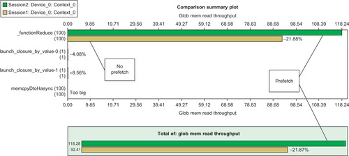
Use of the PTX prefetch instruction clearly benefits larger problems. The reason is that it makes better use of the available global memory bandwidth. Figure 6.2 is a comparison plot created with the visual profiler shows that the prefetch global memory read throughput (the top line) is 21.8 percent higher than the nonprefetch version of the code. The higher global memory read performance benefits larger vector problems, as the prefetch version is always faster than the nonprefetch version. Prefetching is also slightly faster than the thrust implementation, as shown in Table 6.1.
 |
| Figure 6.2 |
The cost of calculating the prefetch address does incur a slight performance penalty over the nonprefetch version for small vector length reductions. Prefetching data is beneficial only when the increased global memory bandwidth lets the kernel run fast enough to overcome the extra costs associated with the prefetch calculation. Keeping the cost of calculating the prefetch indexes is the reason why the example prefetch() functor used such a simple calculation.
Utilizing Irregular Data Structures
The preceding examples utilize very regular access patterns that stream information from global memory.
A large body of computational problems, such as graph and tree algorithms, represents a worst-case scenario for coalescing parallel memory accesses on GPUs. Most of these algorithms exhibit irregular and even random memory access patterns.
Graph algorithms are common in social media analysis (Corley, Farber, & Reynolds, 2011) and, Biology (Jones and Pavel, 2004), and many other fields. Tree algorithms are commonly used for fast data storage and retrieval. Similarly, vector gather and scatter operations are commonly used in sparse matrix and numerical calculations.
A vector gather operation “gathers” data from arbitrary vector elements. See Example 6.17, “A Vector Gather Operation”:
for(int i = 0; i < n; i++) a[i] = b[index[i]];
A vector scatter operation is one that “scatters” data throughout a vector in memory, as in Example 6.18, “A Vector Scatter Operation”:
for(int i = 0; i < n; i++) a[index[i]] = b[i];
Irregular memory accesses are a challenge for massively parallel computers because increasing memory bandwidth does not necessarily increase performance. Coalesced memory accesses imply that memory accesses can be grouped together into a single memory transaction that works on a number of consecutive bytes of information. Table 5.10 and Table 5.11 show the coalesced memory efficiencies for various use cases with caching enabled and disabled on compute 2.0 GPUs.
Irregular memory accesses break the assumption that memory transactions can be coalesced into one or a few large memory transactions. For example, the index vector in Example 6.16 can contain random index values that will cause each thread accessing b[index[i]] to generate a separate global memory transaction. This is a worst-case scenario for the SM (along with the GPU memory subsystem), as each warp will have to wait for all 32 memory accesses to complete before the warp can issue an instruction. In the absolute worst case, all the warps and SM will issue memory transactions that fall on a single memory partition in global memory, which will decrease the available memory bandwidth to that of a single memory subsystem.
The L2 cache in compute 2.0 and later devices provides the best single solution to accelerate algorithms that perform irregular memory accesses. Though not a general solution, the L2 cache will transparently speed most applications just because it provides a high-speed region of memory where the threads on each SM can request small, irregular memory accesses.
Localizing memory accesses can make a tremendous difference in application performance because it allows the L2 cache to work more effectively on behalf of the application threads. Sorting the index array is a reasonable method to use for random data assuming some reordering of the indices is allowed. Of course, much better performance can be achieved when the programmer works to exploit the locality of reference within the algorithm.
The following program, testGather.cu, implements Example 6.16 in a CUDA test code. The thrust API was used to conveniently transfer data to and from the host as well as fill and sort the index array. The first part of the program—Example 6.19, “Part 1 of testGather.cu”—defines a gather functor:
#include <omp.h>
#include <iostream>
using namespace std;
#include <thrust/host_vector.h>
#include <thrust/device_vector.h>
#include <thrust/sort.h>
#include <thrust/sequence.h>
#include <thrust/functional.h>
struct gather_functor {
const int* index;
const int* data;
gather_functor(int* _data, int* _index) : data(_data), index(_index) {};
__host__ __device__
int operator()(int i) {
return data[index[i]];
}
};
Example 6.20, “Part 2 of testGather.cu,” parses the command-line arguments and performs the test:
int main(int argc, char *argv[])
{
if(argc < 3) {
cerr << "Use: size (k) nLoops sequential" << endl;
return(1);
}
int n = atof(argv[1])*1e3;
int nLoops = atof(argv[2]);
int op = atoi(argv[3]);
cout << "Using " << (n/1.e6) << "M elements and averaging over "
<< nLoops << " tests" << endl;
thrust::device_vector<int> d_a(n), d_b(n), d_index(n);
thrust::sequence(d_a.begin(), d_a.end());
thrust::fill(d_b.begin(), d_b.end(),-1);
thrust::host_vector<int> h_index(n);
switch(op) {
case 0:
// Best case: sequential indicies
thrust::sequence(d_index.begin(), d_index.end());
cout << "Sequential data " << endl;
break;
case 1:
// Mid-performance case: random indices
for(int i=0; i < n; i++) h_index[i]=rand()%(n-1);
d_index = h_index; // transfer to device
thrust::sort(d_index.begin(), d_index.end());
cout << "Sorted random data " << endl;
break;
default:
// Worst case: random indices
for(int i=0; i < n; i++) h_index[i]=rand()%(n-1);
d_index = h_index; // transfer to device
cout << "Random data " << endl;
break;
}
double startTime = omp_get_wtime();
for(int i=0; i < nLoops; i++)
thrust::transform(thrust::counting_iterator<unsigned int>(0),
thrust::counting_iterator<unsigned int>(n),
d_b.begin(),
gather_functor(thrust::raw_pointer_cast(&d_a[0]),
thrust::raw_pointer_cast(&d_index[0])));
cudaDeviceSynchronize();
double endTime = omp_get_wtime();
// Double check the results
thrust::host_vector<int> h_b = d_b;
thrust::host_vector<int> h_a = d_a;
h_index = d_index;
for(int i=0; i < n; i++) {
if(h_b[i] != h_a[h_index[i]]) {
cout << "Error!" << endl; return(1);
}
}
cout << "Success!" << endl;
cout << "Average time " << (endTime-startTime)/nLoops << endl;
}
This program requires the user specify:
■ The size of the vector in millions of elements.
■ The number of tests to perform in calculating the average runtime.
■ An integer value that specifies what type of test testGather.cu should perform. The program understands the following values:
■ A 0 value fills the index vector with sequential values. All memory accesses are sequential and coalesced.
■ A 1 specifies that index contains a sorted list of random index values. This option shows the performance that can be achieved by regularizing the index values to exploit any locality.
■ The default is to fill index with random values. This is a worst-case scenario for the GPU memory system.
Running testGather.cu on an NVIDIA C2070 GPU shows that the L2 cache does a remarkably good job when handling small problems. It can provide an order of magnitude of increased performance when the random accesses are localized by sorting. Of course, sorting is good only in the average case. Worst-case performance will not be any different from the random case. This test assumes that index will be reused, so the time to perform the sort was not included in the runtimes reported in Table 6.2.
Sparse Matrices and the CUPS Library
Sparse matrix structures arise in numerous computational disciplines. For many applications, sparse matrix methods are often the rate-limiting methods that dictate application performance. In particular, sparse matrix-vector multiplication (SpMV) represents the dominant cost in many iterative methods for solving large linear systems and eigenvalue problems that arise in a wide variety of scientific and engineering applications.
The CUSP library (Generic Parallel Algorithms for Sparse Matrix and Graph Computations) is a thrust-based project for running sparse matrix and graph computations on the GPU. It provides a flexible, high-level interface for manipulating sparse matrices and solving sparse linear systems. The source code for the library can be downloaded from Google Code, where the project is hosted (http://code.google.com/p/cusp-library/). This library uses a variety of common sparse matrix formats with various advantages, as described in the documentation.
Results in the literature show a compute 1.x GPU can deliver an order of magnitude increased performance over an Intel quad-core Clovertown system (Bell & Garland, 2009). This is an active area of research where people are investigating optimal use of the hardware (El Zein & Rendell, 2011) and sparse matrix representations (Cao, Yao, Li, Wang, & Wang, 2010).
CUSP provides a straightforward interface for sparse matrix operations, as can be seen in Example 6.21, to determine the maximal independent set, which is an independent set that is not a subset of any other independent set. It is an important metric used in social network analysis to identify groups or cliques of people.
#include <cusp/graph/maximal_independent_set.h>
#include <cusp/gallery/poisson.h>
#include <cusp/coo_matrix.h>
// This example computes a maximal independent set (MIS)
// for a 10x10 grid. The graph for the 10x10 grid is
// described by the sparsity pattern of a sparse matrix
// corresponding to a 10x10 Poisson problem.
//
// [1] http://en.wikipedia.org/wiki/Maximal_independent_set
int main(void)
{
size_t N = 10;
// initialize matrix representing 10x10 grid
cusp::coo_matrix<int, float, cusp::device_memory> G;
cusp::gallery::poisson5pt(G, N, N);
// allocate storage for the MIS
cusp::array1d<int, cusp::device_memory> stencil(G.num_rows);
// compute the MIS
cusp::graph::maximal_independent_set(G, stencil);
// print MIS as a 2d grid
std::cout << "maximal independent set (marked with Xs)
";
for (size_t i = 0; i < N; i++)
{
std::cout << " ";
for (size_t j = 0; j < N; j++)
{
std::cout << ((stencil[N * i + j]) ? "X" : "0");
}
std::cout << "
";
}
return 0;
}
Graph Algorithms
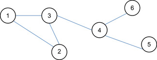
Research on efficient graph algorithm implementations is also an active area of research on GPUs and for parallel computing in general. Instead of using the sparse matrix approach taken by CUSP, these efforts implement a graph data structure composed of nodes and edges. Figure 6.3 shows an example of a labeled graph containing six vertices and edges.
Typical higher-level operations performed on a graph include finding a path between two nodes via either depth-first or breadth-first search and finding the shortest path between two nodes. Graph similarity is an important problem in pattern recognition. For example, chemical compounds can be represented as a graph. In searching chemical databases, it is frequently necessary to compare two graphs to see if they are equal. This leads to interesting computational problems such as how to canonically label a graph for exact search. With a canonical label, it is possible to find graph structures via a string search. Alternatively, graph isomorphism is an important method used to find graphs that have the same or similar structure.
Centrality in a graph is a measure of the relative importance of a vertex within the graph. Examples include: how important a person is within a social network and how critical a road is within a traffic network. The principle centrality metrics are as follows (Corley, Farber, & Reynolds, 2011):
■ Degree centrality: A metric of the connectedness of a node. It is simply a count of the number of edges that attach to a node. For a graph G with n vertices, edges e and vertices v, the degree centrality CD(v) for vertex v is:
(6.1)
■ Closeness centrality: A metric that counts the average distance of a node to all other nodes. Closeness can be productive in communicating information among the nodes or actors in a graph. It is defined in Equation 6.2 as the average shortest path or geodesic distance from node v and all reachable nodes (t in V/v):
(6.2)
■ Betweenness centrality: A metric that measures how often paths between nodes must traverse a given node. Betweenness centrality (Equation 6.3) measures internode influence. In social media analysis, for example, an individual or blog is central if it lies between other individuals or blogs on their geodesics – the blog is “between” many others, where gjk is the number of geodesics linking blog j and blog k (Wasserman and Faust, 1994):
(6.3)
■ Page rank: Page rank (Example 6.4) is an example of eigenvector centrality that measures the importance of a node by assuming links from more central nodes contribute more to its ranking than less central nodes (Brin & Page, 1998). Let d be a damping factor (usually 0.85), n be the index to the node of interest, pn be the node, M(pi) be the set of nodes linking to pn and L(pj) be the out-link counts on page pj:
(6.4)
Certain complex metrics (e.g., betweenness, eigenvector centrality) can become intractable when presented with large volumes of data unless appropriate machines and algorithms are utilized. Developers and users must understand the runtime performance, accuracy, and problem size trade-offs between exact and approximate centrality algorithms (Ediger et al., 2010).
It is possible for a GPU to deliver an order of magnitude or more of increased performance on graph centrality metrics. The gpu-fan (GPU-based Fast Analysis of Networks) project at Vanderbilt provides a working software package that includes methods for computing four shortest path-based centrality metrics. This project reports that the GPU speeds up the application by 10 to 50 times on real-world protein interaction and gene co-expression networks as well as simulated scale-free networks (Shi & Zhang, 2011). The nascent thrust-graph library that is hosted on Google Code is attempting to create a common graph API and set of algorithms for CUDA-enabled GPUs.
Programming graph algorithms on GPUs is in a particularly early stage of development. The paper “Exploring the Limits of GPUs with Parallel Graph Algorithms” (Dehne & Yogaratnam, 2010) is a recent survey of the field. A more dated but still relevant paper is “Accelerating Large Graph Algorithms on the GPU Using CUDA” (Harish & Narayanan, 2007).
SoA, AoS, and Other Structures
Many legacy applications store data as arrays of structures (AoS) that can lead to coalescing issues. From a GPU performance perspective, it is preferable to store data as a structure of arrays (SoA). Example 6.22, “An AoS Example,” creates an AoS:
struct S {
float x;
float y;
};
struct S myData[N];
Arranging data in this fashion leads to coalescing issues as the data are interleaved. Performing an operation that only requires the variable x will result in a 50 percent loss of bandwidth and waste of L2 cache memory.
Example 6.23, “An SoA Example,” shows how to allocate an SoA:
struct S {
float x[N];
float y[N];
};
struct S myData;
Arranging data as an SoA makes full use of the memory bandwidth even when individual elements of the structure are utilized. There is no data interleaving; this data structure should provide coalesced memory accesses and achieve high global memory performance.
The CUDA program sorting_aos_vs_soa.cu is included in the thrust teaching examples that are available for free download from Google Code. It demonstrates how to sort SoA and AoS structures with thrust. The comments in the code note that a 5-times speedup can be achieved by using a SoA data structure.
Tiles and Stencils
The computational grid defined in the kernel execution configuration can be used to break a computation into subproblems that execute in parallel. Tiles and stencils are an abstraction used in the creation of these multidimensional grids. In particular, these abstractions help the programmer group data accesses into common patterns plus define shared memory usage for interthread communications within a thread block.
Matrix multiplication provides the textbook example of the use of 2D regions, or tiles, on the GPU. The book Programming Massively Parallel Processors: A Hands-on Approach (Kirk & Hwu, 2010) has a detailed discussion of matrix multiplication and the use of tiles. However, tiles are a common design paradigm used in many problems aside from matrix multiplication. The CUDA N-body SDK example is another excellent demonstration of the use of tiles to solve a complicated problem on the GPU with high performance.
Stencils are a generalization of the concept of a tile to n dimensions. A stencil computation:
■ Operates on each point in a discrete n-dimensional space.
■ Uses neighboring points in computation.
■ Are often surrounded by a time loop.
■ Can have diverse boundary conditions.
Both tiles and stencils help the CUDA developer formulate problems to best utilize shared memory and register in the SM as well as exploit parallelism across all the SM. The paper “3D Finite Difference Computation on GPUs using CUDA” (Micikevicius, 2010) provides a detailed discussion of stencils that can be freely downloaded from the NVIDIA website. Volkov demonstrates how to use ILP to accelerate stencil problems in “Programming Inverse Memory Hierarchy: Case of Stencils on GPUs” (Volkov, 2010).
Tiles and stencils are also important in performing GPU computations with quadtrees and octrees. A quadtree is a tree-based structure in which each internal node has four children. It is used to partition a two-dimensional space by recursively dividing it into quadrants. An octree has eight children per internal node and is used to recursively divide a 3D space into regions. Both of these data structures can exhibit irregular global memory accesses. The book GPU Computing Gems (Hwu, 2011) contains several detailed examples of how experts in the field have used these and other irregular data structures in CUDA to solve complex scientific problems.
Summary
This chapter introduced techniques and examples to efficiently use GPU memory. The three-orders-of-magnitude performance difference between the slowest and fastest GPU memory systems means that GPU programmers have the opportunity to capitalize on the extreme performance that GPU hardware offers.
What makes CUDA so special is that it exposes the features of the underlying hardware so that the full potential of the hardware can be realized. As the reduction example in this chapter showed, it is possible to delve down into the lowest levels of the hardware execution model to attain high performance.
Thrust, on the other hand, bundled this complexity into a simple API call that was used in the very first program in this book. As demonstrated in this chapter, generic programming lets CUDA programmers create simple, generic methods that fully exploit the capability of the GPU.
Much of the future in CUDA development lies in creating generic libraries and APIs like thrust and CUSP. As these interfaces mature, CUDA programmers will be able to do more in less time. The concept is simple:
■ Make your life easy and write your code with the highest-level API that you feel comfortable using.
■ Profile and see where the bottlenecks occur. In most cases, the efficient use of global memory will likely dominate the application performance.
■ Drop down to a lower-level API to get the performance needed.
■ When possible, write generic methods that can potentially be combined into a generic library for others to use.
..................Content has been hidden....................
You can't read the all page of ebook, please click here login for view all page.