
Multi Field Simulation of Fracture
Luciano Simoni; Bernhard A. Schrefler Department of Civil, Environmental and Architectural Engineering, Padova, Italy
Abstract
We present as areas of interest for multifield fracturing thermomechanical fracturing, fluid pressure induced isothermal and nonisothermal fracturing, fracturing due to radiation, drying, hydrogen embrittlement, and fractures induced by chemical effects. We discuss the most appropriate constitutive models for their simulation and choose the cohesive fracture model for quasi-brittle materials. Successively we show governing equations for a thermo-hydro-mechanical problem, which is representative for multifield problems. Possible extensions to more fields are addressed. Then methods for numerical modeling of multifield fracturing are presented and the most representative ones, i.e., interface and embedded discontinuity elements, X-FEM, thick level set and phase field models, and discrete crack approach with adaptive remeshing are discussed in some detail. After incorporating this last method in the governing equations, their numerical solution is shown together with the necessary adaptivity in time and space. This solution is validated. Successively applications to thermomechanical fracture; hydraulic fracturing in case of a pumped well and of 2D and 3D dams; fracturing of drying concrete and of a massive concrete beam and finally mechanical effects of chemical processes in concrete are shown. In the case of the pumped well with constant pumping rate, a comparison between an Extended Finite Element solution and that of the discrete crack approach with adaptive remeshing is made which allows for interesting considerations about the nature of hydraulic fracturing. The examples permit to conclude that with increasing complexity of the multifield problems that of the employed fracture models decreases, i.e., advanced fracture models have to date only been applied to problems with a limited number of fields, mainly displacement, thermal and/or pressure fields. There is hence plenty of room for improvement.
1 Introduction
Fracturing is a key issue in many multi field problems: they range from thermomechanical fracturing to fluid pressure induced fracturing at isothermal and nonisothermal conditions, fracturing due to radiation or hydrogen embrittlement (corrosion cracking), fracturing induced by chemical effects and others. Materials usually experience reduction of fracture toughness with increasing temperature and a perturbation of the stress state, e.g., induced by loading may trigger the onset of fracturing. This is the case of thermomechanical fracturing. Note that in this case as in several of the subsequent ones the fracture lips are stress free. The situation is different in pressure-induced fracture because there is an interaction between the usually porous solid and the fluid which applies pressure on the fracture lips and in the surrounding process zone: the fracture lips are not stress free. One of the better-known and sometimes questioned applications of pressure induced fracture is hydraulic fracturing or fracking used to open an existing network of microfractures or create a new network in low permeability rocks. This case has deserved much attention because it opened new possibilities of exploiting until now inaccessible hydrocarbon sources (gas and oil) and/or geothermal systems. In the latter case, thermo-hydro-fracturing may be used to make geothermal reservoirs with high temperatures or temperature gradients but low permeability economically exploitable. The extraction of geothermal energy is typically achieved by use of deep wells providing a hydraulic interaction with the hot rock mass. The heat is mined from the reservoir by means of an induced circulation of water between the wells and heat exchange between the reservoir rock and water. A viable fracture network between the wells is hence of paramount importance.
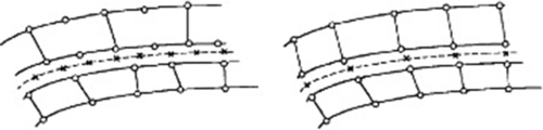
The situation is similar for shale hydrocarbon reservoirs: the low permeability prevented their exploitation till about 1980 when a new technique has been proposed. The first step is drilling a vertical hole down to strata of oil/gas bearing shale (several thousand meters below the surface). When approaching the shale, the drill is redirected horizontally to run for a kilometer or more along the center of the stratum. Eventually explosives are lowered into the horizontal leg to create fractures in the shale and a fluid mixture of water, sand, and chemicals is injected at high pressure fracturing the surrounding rock and releasing the trapped hydrocarbon. Production can then run for years, see Fig. 4.1.

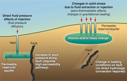
Fracking is often controverted for possible environmental concerns including ground water contamination (e.g., Howarth, Ingraffea, & Engelder, 2011; Vidic, Brantley, Vandenbossche, Joxtheimer, & Abad, 2013), risks to air quality, migration of gases and hydraulic fracturing chemicals to the surface, mishandling of waste, and the health effects of all these, as well as its contribution to raised atmospheric CO2 levels by enabling the extraction of previously sequestered hydrocarbons. An additional concern is that oil obtained through hydraulic fracturing contains chemicals used in hydraulic fracturing, which may increase the rate at which rail tank cars and pipelines corrode, potentially releasing their load and its gases. Another matter of debate is the possibility to induce earthquakes. Hydraulic fracturing routinely produces microseismic events related to drilling operations and mechanical and hydraulic interaction with natural faults (Fig. 4.2). These events are usually much too small to be detected except by sensitive instruments; however, there have been instances of hydraulic fracturing triggering quakes large enough to be felt by people. Usually larger earthquakes are not so much induced by fracturing itself but rather by disposal in deep aquifers of the wastewater from the drilling operations (Ellsworth, 2013; Kerr, 2012). It is obvious that for an unbiased cost-benefit analysis of such important and complex problems reliable mathematical models are a very useful tool.
Overtopping analysis of concrete dams is also an application field of choice of hydraulic fracturing (ICOLD, 1999). Rocks and concrete are so-called geomaterials, i.e., heterogeneous materials of geological origin, which include also soils, bricks, cemented sands, grouted soils, and other cement-based composites. Geomaterials are generally multiphase because of their porous structure and the content of the pore space. Their mechanical behavior depends among others on the pressure level, and can be dilatant under shearing.
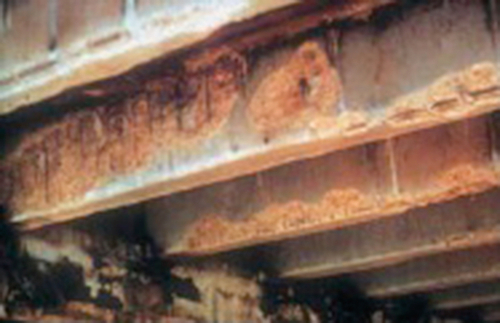
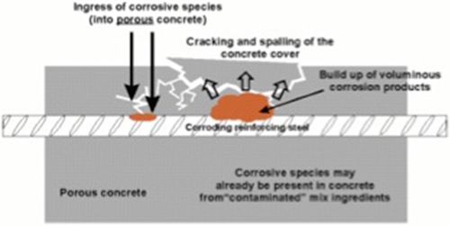
Multifield fracture is of paramount importance for the description of the mechanical behavior not only of geomaterials but also of fiber and particulate composites, coarse-grained or toughened ceramics, ice (especially sea ice), cemented sands, grouted soils, paper, wood, wood-particle board, and biological materials such as bones, intervertebral discs, and similar. The mechanical behavior of such materials and fracture toughness is strongly affected by temperature changes, chemical reactions of the constituents, changes in humidity, aging in addition to the stress effects. We mention here some less known aspects and recall as first example spalling in concrete Figs. 4.3 and 4.4, under severe conditions that occur in a fire. The tensile strength of heated concrete decreases due to dehydration and thermal strains at high temperatures. Moreover, the moisture inside the concrete will evaporate. This combined with the low permeability of high strength concrete will yield high pressures. The pressure can be high enough to cause (violent) cracking and pieces of concrete may chipped off, and in some cases, concrete members can even explode. These phenomena are called spalling. Similar effects can be produced by corrosion of reinforced concrete steel (Fig. 4.5).
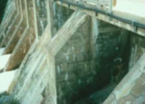
Another example refers to mechanical effects of alkali–silica reactions (ASRs; Figs. 4.6 and 4.7) that is particularly important in large structures such as bridges and dams and can be noticed also on retaining walls.
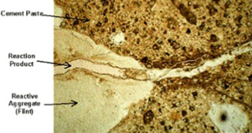
The ASR is usually modeled as a two-stage process; see, e.g., Dunant & Scrivener, 2010, Pesavento, Gawin, Wyrzykowski, Schrefler, and Simoni (2012). In the first stage, the silica present in pores of cement based materials dissolves due to topochemical reactions on the interface of the aggregate and the alkaline solution. Then the dissolved ions are transported by diffusion and advection in the pore solution to microvoids, pores, and cracks in the material skeleton, where the silica reacts with alkali ions, forming an amorphous gel and precipitates. The presence of water is necessary for the process; hence a multifield approach is compulsory for its correct modeling.
During the second phase of the ASR, the amorphous gel, which is strongly hydrophilic, combines with small quantities of water, causing an increase of the amorphous gel volume. After filling up the available pore space, the gel generates an increasing internal pressure in the matrix of cement-based material. The pressure, resulting from water absorption, triggers a significant macroscopic expansion. The water-combination capacity of the hydrophilic gel is altered by an aging effect, which is an intrinsic physicochemical process, independent on the gel formation. The aging process influences both the ASR expansion rate and the final, asymptotic value of the ASR strains. The result of these processes is an increase in tensile stresses and the occurrence of cracks in the paste and through the aggregates in most cases Dunant and Scrivener (2012). For nonstructural concrete applications, ASR is only an esthetic problem. ASR typically manifests efflorescence that stains the surface, causes lots of cracking, may result in faulting and spalling, promotes the entry of chlorides thereby exacerbating corrosion of any reinforcing steel, and is just plain ugly. In structural concrete, ASR is known to reduce strength in cases when harmful expansion is well advanced, lower the modulus of elasticity, and increase creep. Other negative consequences are gel exudation from cracks, misalignment of adjacent sections, closing of joints, extrusion of joint sealant and crushing/spalling of concrete around joints, pop-outs over reactive aggregate particles and operation difficulties (e.g., jamming of sluice gates in dams). Numrical modelling (e.g., Pesavento et al., 2012; Dunant, Bordas, Kerfriden, Scrivener, & Rabczuk, 2011) of these phenomena is a very demending task, with great economical consequences.
As may be seen in the presented cases damaging of the multiphase material may assume two different distributions: very localized fracture or widely distributed microcracking patterns, which start with microseparations. Both types of distribution are, however, linked. Generally speaking microseparations are tiny cracks in the microstructure of the material and their nucleation usually occurs in areas with specific features such as high stresses, sufficiently weak interatomic bonds occurring close to material inhomogeneities as a cavity, or around phase boundaries like an existing crack or a notch. Crack may nucleate also at imperfections on the free surfaces of specimens, locations generally favorable to stress corrosion cracking and fatigue failure for instance in crystalline solids. Energy dissipation in the nucleation process involves friction with ensuing production of heat and plastic permanent deformation of the surrounding bulk material. This nucleation process is irreversible and reduces the stiffness and the strength of the material also when the applied loads are removed. When the applied loads are increased damage increases too and the microcracks can coalesce to form one or more dominant cracks which can lead eventually to the failure of the structure. The evolution from microcracks to failure of the structure differs for each material. From these remarks, it is clear why two different approaches naturally originated in mathematical modeling of the fracturing process: the discrete and smeared crack models respectively. In the first approach, cracks are modeled as discontinuities in the displacement field while in the second approach the displacement field is continuous and the fracturing process is introduced by means of strength and stiffness reduction. Fracture modeling is discussed next in more detail.
2 Fracture Models
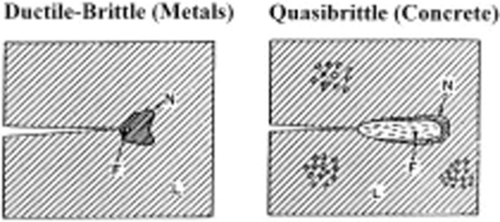
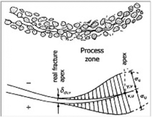
The theoretical and numerical prediction of failure mechanisms due to crack initiation and propagation in solids has ever since been of great importance in engineering starting from the pioneering work of Griffith (1921). Historically, fracture mechanics has been developed mainly for metals, in the frame of linear elastic fracture mechanics (LEFM). Other materials, characterized by a heterogeneous composition, require a fracture mechanics of a different kind from metals. These materials range from geomaterials to fiber and particulate composites, coarse-grained ceramics, ice (especially sea ice), bone, wood, etc. In both metal and the above heterogeneous materials, a sizable nonlinear zone develops at the fracture front. But whereas, in ductile–brittle metals, most of this zone involves hardening plasticity or perfect yielding, and the fracture process zone (FPZ), defined as the zone in which the material undergoes softening damage (tearing), is quite small; in the fracturing process of the mentioned heterogeneous materials the plastic flow is next to nonexistent and the nonlinear zone is almost entirely filled by the FPZ (Fig. 4.8). Such materials are now commonly called quasi-brittle. Further, in multiphase materials, the length of the FPZ, is of the order of the structural size D, understood as the dimension of the cross section (Bažant, 2002).
As pointed out in Bažant (2002) and reported references therein, the scale and size govern almost everything in fracture. In normal concrete or coarse-grained rock, typically the FPZ length l ≈ 0.5 m; in dam concrete with extra large aggregate, l ≈ 3 m, and about the same holds for horizontally propagating fractures in sea ice; in a grouted soil mass, l ≈ 10 m is possible; and in a mountain with jointed rock (with the joints imagined as continuously smeared), l ≈ 50 m may be typical. On the other hand, for drilling into an intact granite block between two adjacent joints, l ≈ 1 cm; in a fine-grained silicon oxide ceramic, l ≈ 0.1 mm, and in a silicon wafer, l ≈ 10–100 nm. Depending on structure size D, different theories are appropriate for analyzing failure. They may be approximately delineated as follows:
| For D/l ≥ 100 | LEFM |
| For 5 ≤ D/l ≤ 100 | Nonlinear quasi-brittle fracture mechanics |
| For D/l < 5 | Nonlocal damage; plasticity |
In the last case, to be more precise, the plastic limit analysis gives only crude engineering estimates of the small-size behavior, while accurate analysis, at least in theory, calls for nonlocal damage models.
LEFM has proven a useful tool for studying fracture problems provided that a flaw-like crack exists in the body and the nonlinear zone ahead of the crack tip is negligible. Even for brittle materials, the presence of an initial crack is needed for LEFM to be applicable. This means that bodies with blunt notches, but no cracks, cannot be analyzed using LEFM. In multiphase materials, the size of the nonlinear zone, most of which coincides with the FPZ, is very large, very often initial cracks are absent, but stress concentrators acting as notches can be found in structural elements. As important example of a multiphase material we refer to concrete: the heterogeneous character of the material promotes crack branching, crack arrest by hard particles and/or by reinforcing bars that is followed by crack nucleation and growth at other locations. Furthermore, a multitude of microscopic initial cracks often grow up due to the exothermal processes that occur during the maturing and hardening of concrete and due to the shrinkage occurring as a consequence of moisture diffusion and the subsequent water loss. These very complex phenomena prevent the use of LEFM, but can be easily accounted for using cohesive models.
2.1 Cohesive Models
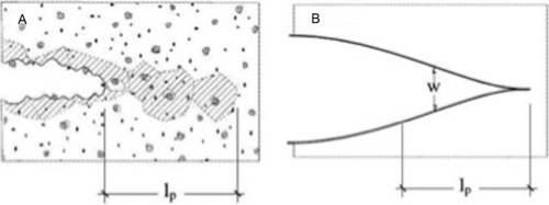
In contrast to conventional engineering fracture mechanics, the cohesive surface methodology permits the analysis of fracture processes in which there is no dominant flaw even though in the original contributions of Barenblatt (1959) and Dugdale (1960) a dominant flaw was assumed present. Hilleborg, Modeer, and Petersson (1976) and Xu and Needleman (1994) extended the cohesive framework to situations without an initial crack. At the moment, the cohesive surface methodology can be assumed as a general model, which, in principle, is applicable to materials other than concrete or cementitious composites; applications in the literature range from crazing in polymers to modeling the effect of strength mismatch in welded joints (Elices, Guinea, Gòmez, & Planas, 2002). Figure 4.9 schematically represents the real situation of the crack, with its nonlinear zone of length l p ahead of crack tip and its mathematical model.
In the cohesive surface formulation, constitutive relations are specified independently for the bulk material and for one or more cohesive surfaces. The cohesive constitutive relation embodies the failure characteristics of the material and characterizes the separation process. The material behaves linear elastically outside the crack. The bulk and cohesive constitutive relations together with appropriate balance laws and boundary (and initial) conditions completely specify the problem. Fracture, if it takes place, emerges as a natural outcome of the deformation process without introducing any additional failure criterion and adequately predicts the behavior of uncracked structures also, including those with blunt notches, not only the response of bodies with cracks (usual drawback of most fracture models).
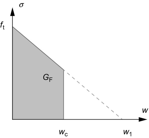
The basic hypothesis of the cohesive crack model is that, for a 2D mode I fracture, the FPZ of a finite width can be described by a fictitious line crack that transmits stress σ normal to the fracture and that this stress is a function of the separation w (called also the opening displacement, or opening width) (Fig. 4.10).
σ=f(w)
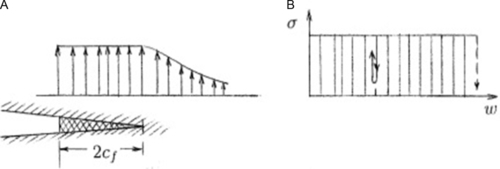
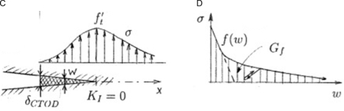
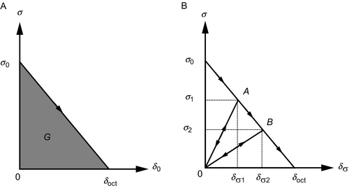
Different possibilities arise for the function f(w), depending on material response: two limiting cases are presented in Fig. 4.10 for ductile–brittle material presented in (A and B) with constant normal stress along the crack and monotonically decreasing stress for quasi-brittle material (C and D). In the latter case, by definition, f(0) = f t′ is the tensile strength of the material. The terminal point of the softening curve f(w) is denoted as wf ; f(wf ) = 0. There is no distinction among an almost formed crack and a micro cracking zone, in which no distinct crack can yet be discerned.
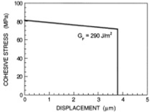
Function f(w) first descends very steeply and then, roughly at σ = 0.15–0.33, f t′ the descent becomes slow (see Fig. 4.11A), with the tail of the descending curve very long. This poses severe problems for the measurement of fracture energy G F, i.e., the area under the entire curve f(w), see Bažant (2002).
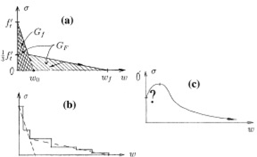
In the initial work of Hilleborg et al. (1976), the softening curve f(w) was described as a decaying exponential with a horizontal asymptote below axis w. Later, simple bilinear forms have generally been adopted (Fig. 4.11A). The important aspect is the representation of the fracture energy; hence, also softening laws as in Fig. 4.11B give virtually the same results with a more complex computational implementation.
Other curves can be found in the literature, the most popular ones are linear, bilinear, power-law, and exponential, although it is possible to implement any other curve. In principle, every type of curve may be considered, but in reality, the choice of a suitable curve and suitable parameters is critical if physical meaningful modeling is desired. The only limitation being that a cohesive zone in a homogeneous body cannot have a hardening branch. As indicated by Elices et al. (2002), assuming a hardening branch followed by a softening one, as in Fig. 4.11C, and an initially homogeneous and isotropic body, we can interpret this limitation in the following way. A cohesive crack starts to open at any given point when the stress at this point reaches f(0). Now, since the stress at this point must increase to further open the crack, this means that the stress at neighboring points must increase too and will thus also exceed f 0, i.e., other cohesive cracks will form and start to open at neighboring points. The resulting picture is that cohesive cracking will extend to a finite zone with infinitely close cracks with infinitely small crack openings, which means that localized cracking is in fact forbidden and what we would get by a consistent use of this model is a behavior of the perfectly plastic type, not of the fracturing type. This means that for cohesive zones in homogeneous bodies the initial stress (the stress required for cracks to start opening) must be the absolute maximum. A monotonically decreasing function is of course a valid case, but a function with a relative maximum less than the initial tensile strength is also acceptable. A function with a secondary maximum larger than the tensile strength would also produce an anomalous behavior in which after a limited opening of a crack other cracks start to open in its immediate neighborhood. The foregoing discussion applies to homogeneous bodies in which the development of a crack is dictated by the stress distribution. A different treatment corresponds to cases where the cohesive zone grows along a preexisting discontinuity, as for example the interface between two elastic blocks jointed by fiber bridging (stitched). In this case, the stress–crack opening curve does not necessarily have to decrease because the cohesive crack (the joint) already exists and does not need to be formed. The only condition to be checked when analyzing this case is that the stresses inside the blocks would not produce cracking outside the joint.
The main parameter in the assumed fracture model is the cohesive fracture energy G F, i.e., the external energy supply required to create and fully break a unit surface area of cohesive crack. It is given by the area under the softening function
GF=∫wf0f(w)dw
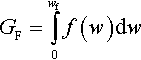
where w f is the critical crack opening, after which the cohesive stress becomes zero.
The area under the entire softening stress-separation curve f(w) represents the total energy dissipated by fracture per unit area of the crack plane, G F, as the crack faces are completely separated at a given point. The area under f(w) also represents the energy dissipated per unit area of crack plane as the FPZ moves forward by a step da (the stress profile σ(x) within the FPZ changing only infinitesimally), as proved by Rice (1968) on the basis of the J-integral. This is theoretically important since it is the latter energy that must be equal to the energy release rate of the structure.
However, in the light of the generally accepted bilinear approximation (Fig. 4.11A) of the softening curve, f(w), it is possible to distinguish two fracture energies: G F defined in Eq. (4.2) and G f, i.e., the area under the initial tangent of f(w), extended down to the w axis
GF=f′2t2σ′0=w02σ′02,σ′0=df(0)dw
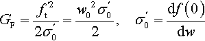
As pointed out by Planas, Elices, and Guinea (1992), within a realistic size range, it is solely G f, which controls the maximum load of a structure and thus this form of softening curve will be assumed in the following.
A further parameter, important for the structural behavior, is the so-called characteristic length. In the light of the above-mentioned distinction in the fracture energy, two definitions of characteristic length can be found
ℓch=EGFf2t,ℓ1=EGff2t=Ew02ft
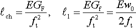
The first can be assumed as an inverse measure of the brittleness of the material (the smaller the l ch the more brittle the material). It is also related to the size of the fully developed FPZ (the size under peak load of the FPZ ahead of a semi-infinite crack in an infinite body). The second is an approximation, which is useful when analyzing the fracture behavior up to and including the peak load, i.e., before much softening takes place anywhere in the body (Elices et al., 2002). Usually the following ratios are accepted:
GF≈2.5Gf,ℓch≈2.5ℓ1
As will be discussed in the following, the characteristic length is of paramount importance also in the numerical solution of the problem.
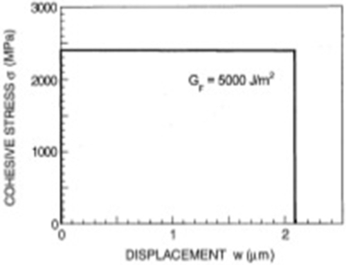
The softening function can be derived either from micromechanical models or from experiments. For an in depth discussion about the characterization of the softening curve from experiment and the related identification process see Bažant (2002) and Elices et al. (2002). In any case, a limited number of parameters are used (three or four, Fig. 4.12). The effectiveness of the cohesive approach has been demonstrated by application outside the geomaterial context, as for PMMA and steel (Fig. 4.13) by proper choice of parameters governing the softening function.
In the case of concrete experimental evidence indicates that the loading rate exerts significant influence on the failure process of the samples, in particular fracture energy increases monotonically with increasing loading rate. Quasi-brittle failure at high strain rates is characterized, in a first stage, by a delay of microcracking growth and in a second stage, by the propagation of many microcracks at the same time. Hence, as pointed out in the introduction, a discrete crack is essentially due to nucleation and growth of microvoids and -cracks. With increasing loading rate, these microcracks do not have sufficient time to search for paths of minimum energy or minimum resistance and are forced to propagate along the shortest path with higher resistance. This suggests that the fracture energy should increase (Rosa, Yu, Ruiz, Saucedo, & Sousa, 2012).
When applying cohesive models the experimentally measured fracture energy G F in mode I is generally used to calibrate the damage evolution law such that the right amount of dissipation will be reproduced. However, it should be reminded that G F comes not only from the creation of surface area (G pF, with “pF” signifies “pure fracture”) but also from friction (G F − G pF). This friction develops from the slips between crack surfaces, and from the pulling out of inclusions. It should further be noted that for some concretes the ratio G pF/G F was in fact estimated to be around 0.25–0.5 (Bažant, 1996). This fact claims for a careful analysis of the displacement field in the process zone: not only has the normal discontinuity w to be controlled, but the relative tangential component too.
2.2 Constitutive Equations for Cohesive Models
We specialize now the constitutive equations of the Section 2.1 for the model of Section 4.7 and applications; they are deemed particularly suitable for multifield problems. Owing that a more complex frame is assumed, in particular as far as opening of new and closing of old fractures is concerned, a new symbology is introduced in the following. Let the complete domain be composed of a set of different homogeneous subdomains. Within a generic one of these, crack nucleation and propagation criterion is determined by the stress state of the solid skeleton. For each homogeneous component, the maximum stress criterion is used: new surfaces are created when the limiting stress value is reached. In a 2D context, these surfaces are oriented in the direction of principal compressive stress, whereas in a 3D context the fracture is supposed to follow the side of the finite element in the apex zone, which is closest to the normal to the plane with maximum tensile stress. The opened lips are assumed as interacting and transmitting tractions as dependent on crack opening, and vanishing when this reaches the critical value
δσcr
![]() (Fig. 4.14). Once this value is exceeded, the only possible tractions for the opposite lips are in compression when closing the fracture reaches a contact position. Between the real fracture apex, which appears at macroscopic level, and the apex of a fictitious fracture extends the already mentioned process zone where cohesive forces act. The constitutive equations below link the cohesive forces to the crack opening along the process zone (Fig. 4.15).
(Fig. 4.14). Once this value is exceeded, the only possible tractions for the opposite lips are in compression when closing the fracture reaches a contact position. Between the real fracture apex, which appears at macroscopic level, and the apex of a fictitious fracture extends the already mentioned process zone where cohesive forces act. The constitutive equations below link the cohesive forces to the crack opening along the process zone (Fig. 4.15).
Within a generic component of the solid skeleton, a fracture can initiate or propagate under the assumption of mode I crack opening, provided that tangential relative displacements of the fracture lips are negligible. In the process zone, cohesive forces are transmitted and are orthogonal to fissure sides. Accounting for the proposals for concrete structures of Hilleborg et al. (1976) and Camacho and Ortiz (1996) the cohesive law is (Fig.4.15)
σ=σ0(1−δσ1δσcr)δσδσ1
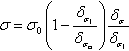
σ
0 being the maximum cohesive traction (closed crack), δσ
the relative displacement normal to the crack,
δσcr
![]() the maximum opening with exchange of cohesive tractions. Following Elices et al. (2002), fracture energy is assumed as
GF=Gf=σ0×δσcr/2
the maximum opening with exchange of cohesive tractions. Following Elices et al. (2002), fracture energy is assumed as
GF=Gf=σ0×δσcr/2
![]() . If the opening velocity changes sign, the cohesive forces are ramped down to zero as the opening displacement itself diminishes to zero, in the spirit of damage mechanics (e.g., Kachanov, 1986), as shown in Fig. 4.15. The individual homogeneous components of the system differ only due to different values attributed to the fundamental parameters of Eq. (4.6) and to the choice of the softening function.
. If the opening velocity changes sign, the cohesive forces are ramped down to zero as the opening displacement itself diminishes to zero, in the spirit of damage mechanics (e.g., Kachanov, 1986), as shown in Fig. 4.15. The individual homogeneous components of the system differ only due to different values attributed to the fundamental parameters of Eq. (4.6) and to the choice of the softening function.
When tangential relative displacements of the sides of a fracture in the process zone cannot be disregarded, mixed mode crack opening takes place. This is usually the case of a crack moving along an interface separating two solid components. In fact, whereas the crack path in a homogeneous medium is governed by the principal stress direction, the interface has an orientation that is usually different from the principal stress direction. As seen above mixed cohesive mechanical model involves the simultaneous activation of normal and tangential displacement discontinuity and corresponding tractions. For the pure mode II tangential effects, the model presented in Fig. 4.16 is used, where the relationship between tangential tractions and displacements is
τ=τ0(1−|δτ1|δτcr)δτ|δτ1|
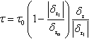
τ
0 being the maximum tangential stress (closed crack), δτ
the relative displacement parallel to the crack and
δτcr
![]() the limiting value opening for stress transmission. The loading/unloading law is also presented in Fig. 4.16.
the limiting value opening for stress transmission. The loading/unloading law is also presented in Fig. 4.16.

For the mixed mode crack propagation, the interaction between the two cohesive mechanisms is treated as in Camacho and Ortiz (1996). By defining an equivalent or effective opening displacement δ and the scalar effective traction t as
δ=√β2δ2τ+δ2σ,t=√β−2|tτ|2+t2σ
the resulting cohesive law is
t=tδ(β2δτ+δσ)
β being a suitable material parameter. The cohesive law takes the same aspect as in Fig. 4.15, by replacing displacement and traction and displacement parameters with the corresponding effective ones.
The presence of water in the multiphase system is handled simply by means of the effective stress concept in the sense of soil mechanics, see Section 3. The same equations as above apply, only that stresses are now the effective stresses in the sense of geomechanics. Also differently from above the fracture lips are no more stress free since the fluid pressure acts on them. For the modification of the cohesive constitutive law for hydrogen embrittlement see Serebrinsky, Carter, and Ortiz (2004). The application of the described cohesive model requires only the discretization of the domain to follow the crack evolution.
3 Governing Equations
Having defined the fracture model, we specify now the governing equations of a typical multifield problem. We refer here to a thermo-hydro-mechanical model, which is sufficiently general to give an idea of how to solve such problems. This model considers a porous solid phase permeated by a fluid phase and a thermal field. It is adequate for nonisothermal cracking (no fluid phase), and for isothermal and nonisothermal hydraulic fracturing. For some geothermal reservoirs where also steam is involved an extension of the model as in Lewis, Roberts, and Schrefler (1989) is sufficient. In case of concrete spalling, the balance equations have to be augmented by a mass balance equation for the gaseous phase composed of dry air and vapor and the enthalpy of phase change has to be included in the enthalpy balance equation (Gawin, Majorana, & Schrefler, 1999; Gawin, Pesavento, & Schrefler, 2003, 2006a, 2006b, 2006c; Zeiml, Lackner, Pesavento, & Schrefler, 2008). The same is true for cracking of drying concrete (Sciumè et al., 2013) and for cracking due to alkali-aggregate reaction, where also a kinetic model for the chemical reaction is needed (Bangert, Kuhl, & Meschke, 2004; Pesavento et al., 2012; Steffens, Li, & Coussy, 2003; Ulm, Coussy, Kefei, & Larive, 2000). The interested reader is referred to the above-cited papers and the references therein. The equations can be obtained by more complete averaging theories such as the Thermodynamically Consistent Averaging Theory TCAT (Gray & Miller, 2014 and Gray, Miller, & Schrefler, 2013). However, for our purpose, the framework of extended Biot's theory in non-isothermal conditions, small displacements and displacement gradients is sufficient. This section is necessarily short and the reader is referred to Lewis and Schrefler (1998) for more detail.
The mechanical behavior of the solid depends on the effective stress σ ij ′ defined, following Biot and Willis (1957) as
σ′ij=cijrs(ɛrs−δrsɛT)−ˉαpδij,ɛT=α3T
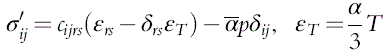
ɛrs
being the total strain tensor, p the fluid pressure, δij
the Kronecker symbol,
ˉα
![]() Biot's coefficient, which accounts for small volumetric strain due to pressure. ɛT
is the strain associated to temperature T changes, according to cubic expansion coefficient α. A Green-elastic material is assumed for the solid at a distance from the process zone, being c
ijrs
the elastic coefficients dependent on the strain energy function W.
Biot's coefficient, which accounts for small volumetric strain due to pressure. ɛT
is the strain associated to temperature T changes, according to cubic expansion coefficient α. A Green-elastic material is assumed for the solid at a distance from the process zone, being c
ijrs
the elastic coefficients dependent on the strain energy function W.
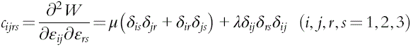
cijrs=∂2W∂ɛij∂ɛrs=μ(δisδjr+δirδjs)+λδijδrsδij(i,j,r,s=1,2,3)
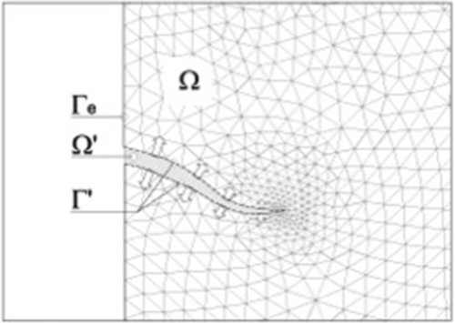
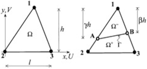
The local linear momentum balance at the generic point of the domain Ω (Fig. 4.17) reads as
σji,j+ρgi=ρ¨uiinΩ
where σij is the total stress tensor, ρ the density of the material mixture, gi the gravity acceleration vector and ui the displacement vector. Dots represent time derivatives. The natural boundary conditions are
σjinj=tionΓandσjinj=cionΓ′
Γ is the external boundary and ti the forced traction, Γ′ the boundary of the process zone and ci the cohesive force. Forced conditions represent fixed displacement along the constrained boundary and completely define the displacement problem. The linear momentum balance for the mixture (solid plus water), in weak form, hence containing the natural boundary conditions, may be written as
∫ΩδɛijcijrsɛijdΩ−∫Ωρδui(gi−¨ui)dΩ−∫ΩδɛijˉαδijpdΩ−∫Ωδɛijcijrsα3δijTdΩ−∫ΓδuitidΓ−∫Γ′δuicidΓ′=0
δɛij is the strain associated with virtual displacement δui .
The local form of water mass balance after incorporating Darcy's law takes the form
(ˉα−nKs+nKw)∂p∂t+ˉαvsi,i−[(ˉα−n)α+nβ]∂T∂t+kijμw(−pj+ρwgj)=0
where n is the porosity, K s and K w the bulk modulus for solid and liquid phases, β the thermal expansion coefficient of water, v i s the velocity vector of the solid phase, kij the permeability tensor of the medium, μ w the dynamic viscosity of water, ρ w its density. Natural boundary conditions are imposed fluxes at the boundary and distinction has to be made between the external boundary Γ and the fracture boundary, as will be discussed below. Forced conditions represent fixed pressure along the constrained boundary.
To complete the mass balance equation for water, we have to specify the permeability tensor. Darcy's law with constant absolute permeability is assumed for the fluid fully saturated medium surrounding the fracture while within the crack Poiseuille or cubic law is assumed to be valid. This is known since a long time in the case of laminar flow through open fractures and its validity has been confirmed in the case of closed fractures where the surfaces are in contact and the aperture decreases under applied stress, the sides remaining parallel. Permeability is not dependent on the rock type or stress history, but is defined by crack aperture only, as stated by Witherspoon, Wang, Iwai, and Gale (1980), in the form
kij=1fw212

w being the fracture aperture; f is a coefficient in the range 1.04–1.65 and takes into account the deviation from the ideal parallel surfaces conditions. In the following, this parameter is assumed as constant and equal to 1.0.
The weak form of the mass balance equation for water in the entire domain Ω (Fig. 4.17) except for the fracture zone is given by
∫Ωδp{(ˉα−nKs+nKw)∂p∂t+ˉαvsi,i−[(ˉα−n)α+ηβ]∂T∂t}dΩ−∫Ω(δp)i[kijμw(−pj+ρwgj)]dΩ+∫ΓeδpqwdΓ+∫Γ′eδpˉqwdΓ′=0
where the test function δp is a continuous virtual pressure distribution satisfying boundary conditions and q
w the imposed flux on the external boundary. In the last term of Eq. (4.17),
ˉqw
![]() represents the water leakage flux along the fracture toward the surrounding medium. This term is defined along the entire fracture, i.e., the open part and the process zone.
represents the water leakage flux along the fracture toward the surrounding medium. This term is defined along the entire fracture, i.e., the open part and the process zone.
Incorporating fluid transport law into the water mass balance equation within the crack results in
∫ˉΩδp{nKw+∂p∂t+∂w∂t−ηβ∂T∂t}dˉΩ−∫ˉΩ(δp)i[w212μw(−pj+ρwgj)]dˉΩ+∫Γ′δpˉqwdΓ′=0
which represents the fluid flow equation along the fracture. In this equation,
ˉΩ
![]() and Γ′ represent the domain and the boundary of the fracture (Fig. 4.17). It should be noted that the last term, representing the leakage flux into the surrounding porous medium across the fracture borders, is of paramount importance in hydraulic fracturing techniques. In the present formulation, this coupling term does not require special assumptions, as in Boone and Ingraffea (1990), for instance. It can be represented by means of Darcy's law using the permeability of the surrounding medium and pressure gradient generated by the application of water pressure on the fracture lips.
and Γ′ represent the domain and the boundary of the fracture (Fig. 4.17). It should be noted that the last term, representing the leakage flux into the surrounding porous medium across the fracture borders, is of paramount importance in hydraulic fracturing techniques. In the present formulation, this coupling term does not require special assumptions, as in Boone and Ingraffea (1990), for instance. It can be represented by means of Darcy's law using the permeability of the surrounding medium and pressure gradient generated by the application of water pressure on the fracture lips.
Heat transfer is addressed next. The local form of energy balance equation (first law of thermodynamics), under the assumption of small strains requires that
ρ˙e=σij˙ɛij+ρr−qj,j
where e is the specific internal energy, r is the strength per unit mass of a distributed internal heat source, and qj the heat flux vector. Forced conditions fix the temperature along the boundary, whereas natural conditions represent the imposed heat flux. The latter includes also the convective heat transfer toward the surrounding. Both fluxes will be defined by means of suitable constitutive models.
Fourier's law is used as constitutive assumption for heat flux (λij being the effective thermal conductivity tensor), and Newton's law to represent convective flux (being h the convective heat transfer coefficient and T∞ the temperature in the far field of the undisturbed surrounding.
qi=−λijTj,qconvi=h(T−T∞)
In a generic thermodynamic problem, for an infinitesimal increment of deformation, the specific internal energy can be assumed as a function of absolute temperature, a set of observable variables (the displacement field) and internal variables vi (Lemaitre & Chaboche, 1990). For the application of Section 6.2, we assume that mechanical terms in energy balance equation are negligible compared with thermal effects. This is not always the case. Sometimes, in experimental investigations a significant temperature increase has been observed in the zone of crack initiation and propagation (Guduru, Zehnder, Rosakis, & Ravichandran, 2001). To account for these situations, dissipation terms related to mechanical effects have to be introduced in the energy balance equation, following (Rice & Levy, 1969) for instance.
When mechanical terms are neglected, internal energy depends on temperature only and is related to heat capacity of the mixture at constant volume C v. Volume heat sources s are retained, because they can represent very different phenomena, e.g., heat production due to hydration of concrete or to plastic work, if included. Hence they represent coupling effects between stress and thermal fields. Source terms may also arise along the boundary and represent frictional effects. In particular, the rate at which heat is generated at the contact surfaces is
r′=t⋅||v||
where t is the contact traction and ||v|| is the jump in velocity across the contact. This effect can be incorporated in the weak form of the energy balance, which hence takes the form
∫Ωρ(Cv˙T)θdΩ+∫Γ′r′θdΓ′+∫Γ′qconvθdΓ+∫Γ′qθdΓ=∫ΩqdivθdΩ+∫ΩsθdΩ
being θ an admissible virtual temperature, q conv and q the convective and imposed heat flux normal to the boundary.
For the model closure, the initial conditions are needed that specify the full fields of primary state variables and internal variables at time instant t = 0, in the whole analyzed domain Ω and on its boundary Γ
u=uo,p=po,T=To,˙u=˙uo,onΩ∪Γ
The governing Eqs. (4.14), (4.17), (4.18), and (4.22) have to be discretized in space by means of the Galerkin procedure with continuous interelement approximation and in time (usually but not necessarily in this order) and the resulting algebraic system is solved to obtain the displacement vector, pressure, and temperature fields together with the fracture path. In fact, with the evolution of the fracture we have a continuous change of the domain and boundary topology. In particular, the fracture path, the position of the process zone and the cohesive forces are usually unknown and must be determined during the analysis. The problem is emphasized by the necessity of coupling fields with very different time scales, which are governed by the transport laws. Several strategies can be found in the literature for solving the fracturing aspect, which are discussed in the Section 4. They often refer only to a subset of the presented equations. It is clear that by reducing the complexity of the field problem, less sophisticated procedures may become viable and/or efficient. Sometimes, a procedure is defined effective and useful for instance only on the basis of reduction of computational costs, without accounting for the reduction of the accuracy of the solution itself, which could be necessary for a correct resolution of a coupled field. This aspect will be discussed in Section 7.
4 Numerical Approaches to Fracturing
4.1 Review of Numerical Solution Strategies
Before discussing in detail numerical solution strategies, we present a short overview of what can be found in literature. Many of the papers deal with hydraulic fracturing because it is the most common multifield fracturing problem. Contributions to the mathematical modeling of fluid-driven fractures have been made continuously since the 1960s, beginning with Perkins and Kern (1961). These authors made various simplifying assumptions, for instance regarding fluid flow, fracture shape and velocity leakage from the fracture. For other analytical solutions in the frame of linear fracture mechanics, assuming the problem to be stationary, see Rice and Cleary (1976), Cleary (1978), Huang and Russel (1985a), Huang and Russel (1985b), Detournay and Cheng (1991). These papers suffer the limits of an analytical approach, in particular the inability to represent an evolutionary problem in a domain with a real complexity. An analysis of solid and fluid behavior near the crack tip can be found in Advani, Lee, Dean, Pak, and Avasthi (1997) and Garagash and Detournay (2000). Boone and Ingraffea (1990) present a numerical model in the context of linear fracture mechanics, which allows for fluid leakage in the medium surrounding the fracture and assumes a moving crack depending on the applied loads and material properties. Tzschichholz and Herrmann (1995) used a 2D lattice model for constant injection rate in homogeneous and heterogeneous materials, which only break under tension. Carter, Desroches, Ingraffea, and Wawrzynek (2000) show a fully 3D hydraulic fracture model, which neglects the fluid continuity equation in the medium surrounding the fracture. Serebrinsky et al. (2004) have studied hydrogen embrittlement (corrosion cracking) with a cohesive model of fracture, which accounts for the effect of impurity segregation. The cohesive law is integrated into the calculations by means of six-node cohesive elements (Ortiz & Pandolfi, 1999) and the mechanical model is coupled with a diffusion equation for hydrogen. A discrete fracture approach with remeshing in an unstructured mesh and automatic mesh refinement is used by Secchi, Simoni, and Schrefler (2004) for cohesive fracturing in a thermo elastic bimaterial and by Schrefler, Secchi, and Simoni (2006) to fluid pressure induced fracturing. This approach has been extended to 3D situation by Secchi and Schrefler (2012) and will be discussed in more detail in Sections 4.7 and 5. Interface elements in combination with remeshing techniques were used by Khoei, Barani, and Mofid (2010) for fracturing processes in saturated porous media under dynamic conditions. Carrier and Granet (2012) develop a zero-thickness finite element to model a fluid pressure driven fracture in a permeable poroelastic medium. The fracture propagation is governed by a cohesive zone model and the flow within the fracture by the lubrication equation. A mixed mode cohesive model was chosen to represent the process zone.
Partition of unity properties of finite element shape functions (PUFEM) have been applied to hydraulic fracturing in a partially saturated porous medium by Réthoré et al. (2008) in a 2D setting. In this case, a two scale-model has been developed for the fluid flow: in the cohesive crack Darcy's equation is used for flow in a porous medium and identities are derived that couple the local momentum and mass balances to the governing equations for the unsaturated medium at macroscopic level. PUFEM were also applied by Kraaijeveld & Huyghe (2011) together with both a strong and a weak discontinuity model for flow and Kraaijeveldt, Huyghe, Remmers, and de Borst (2013) for 2D mode I crack propagation in saturated ionized porous media. Mohammadnejad and Khoei (2013a, 2013b) solve the hydraulic fracturing problem with X-FEM, using full two phase flow throughout the region. Darcy flow is assumed within the crack. Phase fields with regularization of a sharp crack topology by a diffusive crack topology also appeared recently as an interesting approach in the field of hydraulic fracturing. Damage models were used for simulation of concrete spalling by Witek, Gawin, Pesavento, and Schrefler (2007), for alkali–silica reaction in concrete by Pesavento et al. (2012) and for cracking due to aging in concrete by Sciumè et al. (2013).
However, there are not only smeared models and discrete crack models in a continuum, but also discrete element approaches. The distinct element method DEM is used by Eshiet and Sheng (2011). The model is made up of an assembly of rigid randomly sized and arbitrary shaped particles interacting with other particles at interfaces or at the point of contact between them. The fluid domain is composed of the voids surrounded by particles connected by pipes representing a particle contact (Al-Busaidi, Hazzard, & Young, 2005). Fluid flow through the pipes is modeled with a cubic law for flow and the Parallel Plate Model (modified Poiseuille law). Pressure exerted on particles by the fluid in the domain causes deformation and displacement of the particles which alter the contact forces used to update the aperture size of the channels. The fluid–solid coupling is hence guaranteed via changes in aperture as a result of contact forces; changes in domain pressures as a result of changes in domain size; and the exertion of domain pressure on surrounding particles.
Another discrete approach is the particle finite element method (PFEM) which is used for analysis of complex coupled problems in mechanics involving fluid–soil–structure interaction (Oñate et al., 2004, 2011). The PFEM uses an updated Lagrangian description to model the motion of nodes (particles) in both the fluid and the solid domains (the later including soil/rock and structures). A mesh connects the particles (nodes) defining the discretized domain where the governing equations for each of the constituent materials are solved as in the standard FEM. This method is potentially useful for multifield fractures but no applications for this have been shown. For fluid structure interaction problems see Idelsohn, Oñate, del Pin, and Calvo (2006).
Numerical approximations alternative to the conventional finite element technology for deformable fluid-saturated porous media have been recently presented by Irzal, Remmers, Verhoosel, and de Borst (2013) and Shahrokhabadi, Vahedifard, and Ghazanfari (2014) in the frame of isogeometric analysis (IGA) that uses nonuniform rational B-splines. The ability of these functions is not only to exactly represent complex geometries, but also to provide higher order continuity and more regular field variables approximations with ensuing additional advantages in the preservation of local mass balance equations. In the context of isogeometric analysis, an interface element has been presented by Irzal, Remmers, Verhoosel, & de Borst, 2014 that is based on the isogeometric analysis concept. Through Bézier extraction, this interface element can be casted in the same format as conventional interface elements. An interesting property of the isogeometric approach is the possibility to increase the interelement order of continuity, but, when needed, to locally reduce this continuity in a very straightforward way. Isogeometric interface elements inherit the simplicity of conventional interface ones, but also some deficiencies, such as the occurrence of traction oscillations when high interface stiffness is used. The approach is very promising, also for the computational very simple refinement capabilities.
Meshless (or mesh-free methods) are another class of methods that have successfully emerged to treat crack problems. A recent review, including computer implementation aspects, is provided in Nguyen, Rabczuk, Bordas, and Duflot (2008). A review of partition of unity methods for fracture applications is provided in Rabczuk, Bordas, and Zi (2010) and Rabczuk, Zi, Bordas, and Nguyen-Xuan (2010). The basic idea behind meshless methods is to relax the constraints imposed upon meshes by mesh-based methods, in particular, with respect to the connectivity between nodes and elements. The approximation is built based on a cloud of points (nodes) related to each other by influence functions.
A number of approaches are available in meshless methods to treat discontinuities. Historically, the first methods used enrichments, which were “intrinsically” embedded within the vector of monomials of the mesh-free approximations. Later, partition of unity enrichment appeared, which allowed to localize the enrichment where and only where it is needed. More recently, methods based on the enrichment of the weight (influence function) appeared, e.g., Duflot and Nguyen-Dang (2004a, 2004b), Duflot (2006), and Muravin and Turkel (2006) and more recently in Barbieri, Petrinic, Meo, and Tagarielli (2012) and Barbieri and Petrinic (2013).
One of the key difficulties when modeling fracture using a discrete crack approach is to maintain crack path continuity and handle merging and intersection of various cracks, which is automatically dealt with in thick-level set methods and phase field models (PFM; see Sections 4.5 and 4.6), which automatically deal with intersection, branching, and merging, without any special treatment. In mesh-free methods, these difficulties are still present, in particular, when the cracks are handled implicitly, i.e., through some type of enrichment of the basis functions. To simplify the treatment of numerous and branching cracks, a class of methods known as “cracking particle methods” was put together (Rabczuk & Belytschko, 2004), which suppresses the need to deal with crack path continuity. In addition, it was shown in Rabczuk, Zi, Bordas, and Nguyen-Xuan (2008), Rabczuk, Bordas, et al. (2010), and Rabczuk, Zi, et al. (2010), Bordas et al. (2008) that crack path continuity can be maintained, even for large numbers of cracks, in statics, dynamics, for linear and for nonlinear materials and large deformations. The methods were also extended to shear bands Rabczuk, Areias, and Belytschko (2007a, 2007b).
Meshless methods have the advantage of providing easily high-order continuity to the basis functions, thus leading to smooth gradient fields in the vicinity of the crack fronts and, consequently, to accurate computations of the fracture parameters governing crack growth. Examples of these features are developed in the work of Duflot and Nguyen-Dang (2002, 2004a, 2004b), Zhuang, Augarde, and Bordas (2011), and Zhuang, Augarde, and Mathisen (2012) for linear elastic fracture and fatigue, where the accuracy in the computation of the stress intensity factors is of critical importance.
Meshless methods have also been developed for multifield problems. A few examples of such developments include magneto-electro-elastic effects, Sladek, Sladek, Solek, and Pan (2008), shear band propagation, Li, Liu, Rosakis, Belytschko, and Hao (2002), and thermoelastic wave propagation, Akbari, Bagri, Bordas, and Rabczuk (2010). Developments related to multifield fracture are also available, but scarcer, for example, failure in piezoelectric materials, e.g., Sladek, Sladek, Zhang, Solek, and Starek (2007) and magneto-electro-static solids in Sladek et al. (2008).
PFM, as described in Section 4.6, can of course also be set within a meshless framework or within an isogeometric framework, with which meshless methods have a number of similarities, e.g., Nguyen, Bordas, and Rabczuk (2013), including high-order continuity, which is particularly useful for high-order partial differential equations and level set approximations as required in the thick-level set method and PFM. It is thus not surprising that such models were also developed for fracture, for example, in thin shells, e.g., Amiri, Anitescu, Arroyo, Bordas, and Rabczuk (2014) and Amiri, Millán, Shen, Rabczuk, and Arroyo (2014).
In order to create bridges between the extended finite element method and the (extended) mesh-free/meshless methods, a number of alternatives were proposed recently, for example, relying on enriched maximum entropy interpolants (Amiri, Anitescu, et al., 2014; Amiri, Millán, et al., 2014) and through gradient smoothing (the smoothed extended finite element method), which originates from stabilized conforming nodal integration, first introduced within the realm of mesh-free methods by Chen, Wu, Yoon, and You (2001) and which provides the (X)-FEM with insensitivity to mesh distortion and locking (see Bordas, Rabczuk, Hung, et al., 2010; Bordas, Rabczuk, Ródenas, et al., 2010 for a recent review).
The smoothed X-FEM (Bordas et al., 2011; Chen et al., 2012; Vu-Bac et al., 2011) and smoothed FEM (Jiang, Tay, Chen, & Sun, 2013; Liu, Chen, Nguyen-Thoi, Zeng, & Zhang, 2010) have been used for crack propagation in linear elastic solids and for multifield problems (e.g., Nguyen-Van, Mai-Duy, & Tran-Cong, 2008; Nguyen-Xuan, Liu, Nguyen-Thoi, & Nguyen-Tran, 2009; Phung-Van, Nguyen-Thoi, Le-Dinh, & Nguyen-Xuan, 2013).
We eventually recall applications of the Boundary element method to multifield fracture problems, for instance Behnia, Goshtasbi, Fatehi Marji, and Golshani (2011), who analyzed crack propagation due to hydraulic fracturing, Ganis, Mear, Sakhaee-Pour, Wheeler, and Wick (2014) for the modeling of fluid injection and reservoir simulation, Castonguay, Mear, Dean, and Schmidt (2013) for growth and interaction of multiple hydraulic fractures in three dimensions, together with the cited references therein.
Boundary element methods (BEMs) are particularly attractive when dealing with fracture, because such methods require only the generation and regeneration of a boundary mesh. They are, however, restricted to cases where fundamental solutions can be derived. The recent work of Simpson and Trevelyan (2011a, 2011b) on enriched boundary element methods (XBEM) proposes, for the first time to use the partition of unity enrichment concept within a boundary element framework. This work is not available yet for multifield problems. As long as the PDEs remain linear and their coupling as well, there is no inherent difficulty preventing such extensions (see for example Giannopoulos & Anifantis, 2007, for a BEM treatment of thermomechanical interfacial fracture including contact and friction). However, if any nonlinearity is introduced, either in the coupling between the PDEs or in the PDEs themselves, which is the general case, BEMs may lose their boundary nature and require a background mesh.
The isogeometric BEM and the GIFT (geometry-independent field approximation) framework were developed recently and allow damage tolerance assessment, crack growth simulation, and shape optimization, directly from computer aided design (CAD) data without any mesh generation (see Lian, Simpson, & Bordas, 2013; Scott et al., 2013; Simpson, Bordas, Lian, & Trevelyan, 2013; Simpson, Bordas, Trevelyan, & Rabczuk, 2012). This work has not yet been extended to cover multifield problems. A recent review on the simplification of CAD-analysis transition, including discussions on alternate methods based on implicit boundary definitions and NURBS-enhanced finite element methods is presented in Lian, Bordas, Sevilla, and Simpson (2012), Bordas, Rabczuk, Hung, et al. (2010), and Bordas, Rabczuk, Ródenas, et al. (2010).
Independently of the particular strategy adopted, a key point is the reliability evaluation of the solution. Disregarding model errors (geometry and material modeling), which are not the scope of this chapter, we recall here some basic results on a posteriori error estimation in numerical simulation. For a general discussion on their sources, we refer to Ainsworth and Oden (1997) and Lewis and Schrefler (1998). Once the model error is controlled, the next step is to minimize the discretization error, i.e., the error committed by approximating the solution of the problem, which lives in an infinite dimensional space, by a finite dimensional subspace, usually polynomial, but which, within the realm of enriched methods, can also include nonpolynomial basis vectors, singularities, and discontinuities.
There are several difficulties associated with the evaluation of the discretization error, which are compounded by the existence of fractures (geometrical features involving discontinuities and possible singularities). The key concept behind recovery-based error estimators is to construct an enhanced solution from the raw solution provided by the numerical simulation. This recovered/enhanced solution is usually constructed by smoothing the raw solution and this smoothed solution may be further constrained to satisfy equilibrium and compatibility conditions. An excellent monograph on the topic is by Ainsworth and Oden (1997).
Some of the more often used or promising methods for fracturing in multi field problems are now discussed in some detail.
4.2 Smeared and Discrete Crack Approaches
Smeared and discrete crack theories start from the notion of a continuum and a discontinuum respectively. In the smeared crack approach, the nucleation of one or more cracks in the volume that is attributed to an integration point is transformed into a deterioration of the current stiffness and strength for the corresponding element. When the combination of stresses at that integration point satisfies a specified fracture criterion, a crack is initiated. In a 2D context, this implies that when stress, strain, and history variables are monitored, the isotropic stress–strain relation is replaced by an orthotropic elasticity-type relation with the axes of orthotropy normal to the crack and tangential to the crack. Upon cracking, both the normal stiffness and the shear stiffness across the crack are set equal to zero.
Within the smeared crack formulation a distinction is furthermore made between fixed, multidirectional, and rotating cracks, whereby the orientation of the crack respectively is kept constant, updated in a stepwise manner or updated continuously.
Although the cohesive surface model is essentially a discrete approach, it can be transformed into a smeared formulation by distributing the fracture energy over the volume in which the crack localizes.
In general, the resulting material stiffness is represented by ill-conditioned matrices, hence, can induce convergence difficulties. Further, setting the stiffness normal to the crack equal to zero gives a sudden drop in stress from the tensile strength to zero on crack initiation. This can cause numerical problems as well.
Finite element models with embedded discontinuities (Section 4.3) provide an elegant way to implement smeared-crack models. Indeed, the embedded discontinuity approaches enhance the deformational capabilities of the elements, especially when the standard Bubnov–Galerkin approach is replaced by a Petrov–Galerkin method, which properly incorporates the discontinuity kinematics. At the expense of obtaining a nonsymmetric stiffness matrix, the high local strain gradients inside crack bands are captured more accurately. However, a true discontinuity is not obtained because the kinematics of the embedded crack band is diffused over the element when the governing equations are cast in a weak format, either via a Bubnov–Galerkin or via a Petrov–Galerkin procedure. Indeed, it has been shown that the embedded discontinuity approaches and conventional smeared crack models are equivalent. Consequently, the embedded discontinuity approaches inherit many of the disadvantages of conventional smeared crack models, including the sensitivity of crack propagation to the direction of mesh lines (de Borst, Remmers, Needleman, & Abellan, 2004).
The results for the various crack formulations show large discrepancies. Smeared cracks may give rise to stress locking while discrete cracks do not. Fixed smeared cracks may produce overstiff behavior while rotating smeared cracks do not. Also, physically unrealistic and distorted crack patterns may be obtained (Peerlings, de Borst, Brekelmans, & Geers, 2002).
Continuum damage models, including the class of smeared crack models suffer from loss of ellipticity beyond a certain level of accumulated damage. As a consequence, the rate boundary value problem ceases to be well posed, which typically results in an infinite number of possible solutions. A numerical solution just “picks” a solution from this available solution space, which results in an excessive mesh dependency.
To regularize the solution, higher order continua have been proposed. In the context of damage models, nonlocal models in an integral format or in a differential format have been put forward. Anisotropic versions of gradient models have been published as well (Kuhl, Ramm, & de Borst, 2000).
With the aim of a discrete representation of cracks within a continuum setting of the FEM different approaches have been pursued, which permit the representation of cracks as embedded discontinuities within finite elements, circumventing the need for remeshing as cracks evolve. The framework of these methods is the partition of unity method (PUM), proposed by Babuška and Melenk (1997), which allows for the construction of conforming ansatz spaces, with local properties determined by the user. The development of this method was motivated by the need for new techniques for the solution of problems where the classical FEM approaches fail or are prohibitively expensive; for example, equations with rough coefficients (arising, e.g., in the modeling of composites, materials with microstructure, stiffeners, etc.) and problems with boundary layers or highly oscillatory solutions fall into that category. The PUM offers the possibility to include arbitrary enhancement functions into the finite element approximation. The approach taken in the PUM is to start from a variational formulation and then design the trial (and test) spaces in view of the problem under consideration. The main features of the PUM are twofold: the inclusion of a priori knowledge about the differential equation in the ansatz spaces and the possibility to construct easily ansatz spaces of any desired regularity; therefore, trial spaces for the use in variational formulations of higher order differential equations (e.g., various plate and shell models) are available.
Depending on the way the ansatz is constructed, specific names may be used, as embedded crack models (see Section 4.3) and nodal-based formulations, e.g., the Extended Finite Element Method (X-FEM; see e.g., Dumstorff & Meschke, 2007; Khoei, Barani, & Mofid, 2011 for porous media problems). With the exception of the “rotating” crack formulation of the strong discontinuity approach, the topology of crack segments is held fixed once they are signaled to open.
4.3 Interface Elements and Embedded Discontinuity Elements
In the frame of FEM, discontinuities in the displacement field caused by damage localization and fracture can be easily accommodated along the boundaries of elements defined by independent nodes, see in Fig. 4.18 (Bolzon & Corigliano, 1997). Interface laws and relevant discretization rules define the connection ties that reproduce perfect continuity, cohesion, or full separation in numerical simulations. This approach is rather effective when the fracture path or the direction of the localization bands are known in advance. Otherwise, the results can be severely biased by the discretization, in terms of material separation paths and of overall dissipation. A dummy stiffness has to be introduced to prevent the crack from debonding when it is not physical (de Borst et al., 2004).
Xu and Needleman (1994) placed interface elements between all continuum elements in the finite element mesh and were able modeling complex fracture phenomena such as crack branching or crack initiation away from the crack tip. The drawback of placing interfaces between all continuum elements is that the process is not completely mesh independent, because the crack path is aligned with element boundaries. Moreover, a too weak dummy stiffness generates flexible results and a too strong dummy stiffness can cause numerical problems like traction oscillation at the cohesive surfaces (de Borst et al., 2004; Schellekens & De Borst, 1993).
The problem of interface elements can be overcome by considering elements enhanced by a discontinuous contribution to the displacement field across embedded interfaces, which are progressively activated as shown for instance in Fig. 4.19 (Bolzon & Corigliano, 2000).
The displacement field at element level is therefore described by the sum of a regular contribution, described by standard shape functions and nodal degrees of freedom, and by a discontinuous one, which has been defined in different ways. An overview can be found for instance in Dias-da-Costa, Alfaiate, Sluys, Areias, and Júlio (2013).
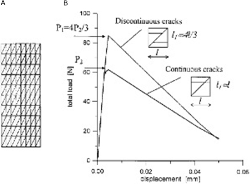
In some proposals, the discontinuity locus is represented by a straight segment crossing the centroid of the element, often defined only for the master square in the parent space, and/or a uniform displacement jump is defined at the element level. Thus, the enhanced displacement field cannot generally satisfy interelement compatibility, tractions are discontinuous across the element boundaries and dissipation is not correctly evaluated. These limitations are evidenced for instance in Figs. 4.20 and 4.21 (Bolzon & Corigliano, 2000), which visualize the simulation results of simple tension tests performed on homogeneous or reinforced plates. The embedded interfaces are activated at the fulfillment of a stress-based criterion frequently adopted in quasi-brittle fracture, which also controls the evolution of the displacement discontinuities.

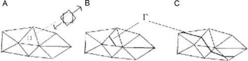
Interelement conformity is achieved by introducing additional nodes and degrees of freedom, shared with the adjacent elements, in correspondence of the newly forming interfaces, as shown for instance in Fig. 4.22 (nodes A and B in the CST, nodes i and j in the quadrilateral). The sequence of activation is carefully controlled and the last introduced node identifies the crack tip. The crack tracking procedure is nonlocal in the case of quadrilateral elements, because it is necessarily evaluated on averaged values of the stress distribution.
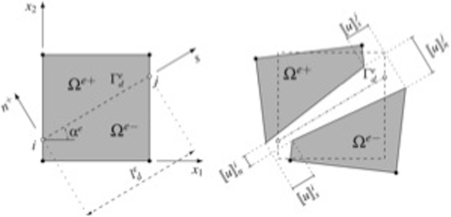
The enhanced displacement field at element level can be expressed by the sum of the contributions:
u(x)=Nu(x)U+N±w(x)W±
where vector U collects the nodal displacements of the standard element while W± represent the additional degrees of freedom, associated to the displacement jumps
W=W+−W−
The relevant shape functions, N w ±, share the same properties of the standard ones, N u , but are defined in the subdomains Ω + and Ω –, see Fig. 4.22. Thus enriched, even the simple CST becomes rather effective.
Once inserted within the equilibrium equations, expressed in weak form by the principle of virtual work, Eq. (4.24) give rise to an equation system of the form
[KuuK+uwK−uwK+wuK+ww0K−wu0K−ww][UW+W−]=[PuP+wP−w]−[0T−T]
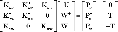
The right hand side of the system (4.26) represents the vectors of equivalent nodal forces, where T vector indicates the nodal forces associated to the embedded interface and usually governed by the assumed cohesive law.
In most approaches, the additional degrees of freedom at the interface (W± with the above notations) are condensed at the element level before overall assembly. Thus, the final formulation and the corresponding results are very similar to those resulting from standard displacement-based finite element and smeared crack approaches. The corresponding output, shown for instance in Fig. 4.21, does not permit to appreciate possible conformity violation. On the contrary, maintaining the additional degrees of freedom produces results, which are free of the above limitation and consistent with the discrete-crack idealization; see e.g., Fig. 4.23 (Dias-da-Costa et al., 2013). Static condensation can be exploited to reduce variables to interface degrees of freedom (displacement discontinuities and tractions) only. This solution strategy, unconventional in FE approaches but rather common in the boundary element context, is particularly convenient from a computational point of view when a linear background is considered (small displacement and linear elasticity outside the progressive-forming interfaces), typical of quasi-brittle fracture problems.

4.4 Extended Finite Element Method
The X-FEM method is characterized by the incorporation of discontinuous shape functions into the finite element approximation, as has been suggested first in the pioneering work of Dvorkin, Cuitino, and Gioia (1990) and by exploiting the partition of unity property of the finite element shape functions by Babuška and Melenk (1997). Cracks are not limited to element boundaries but can be located arbitrarily in the finite element mesh and allowed to continuously propagate through elements. Considering for the moment only the solid field, to improve the ansatz, a crack tip function can be introduced to enhance the resolution of the displacement field approximation in the vicinity of the tip.
These approaches have been used both for LEFM, where stress field in the vicinity of the tip exhibit a singularity, and in cohesive formulation, where crack tip functions do not exhibit stress singularities but yield bounded values of stresses. In zones of crack opening, the transfer of residual stresses parallel as well as orthogonal to the crack faces after crack initiation must be represented by an adequate traction separation law considering interactions between shear and normal components of crack displacements and interface tractions in mixed-mode situations. In the areas where no tractions are transmitted between the lips of the fracture, appropriate discontinuous functions must be introduced to enrich the displacement field. Heaviside and Sign functions represent useful tools to this end. Using enhancement functions for cracks fully penetrating elements and for the crack tip located within elements, cracks may continuously propagate through elements and are not restricted to elements edges. This enables also modeling of curved cracks within elements. This approach can be used indifferently with structured and unstructured meshes. For a more detailed and complete description of the method we refer to Moës, Dolbow, and Belytschko (1999), Wells and Sluys (2001), Moës and Belytschko (2002), Remmers, de Borst, and Needleman (2003).
In order to model the presence of the discontinuity, the usual polynomial finite element approximation may be enriched by one or two additional terms. In general, we can assume
uh=∑i∈IuiNi+∑j∈JbjNjH(f(x))+∑k∈KNk(∑l=1clkFl(x))
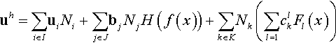
where I is the set of all nodes in the mesh; u i is the usual vectorial displacement degree of freedom at node i and Ni is the shape function associated with node i. Each shape function Ni has compact support given by the union of the elements connected to node i. The first additional term involves the jump Heaviside function and f(x) is the signed distance function to the crack (the sign determining whether x is on one side or the other of the crack). The nodes enriched by the function H are such that their support (we mean the support of the nodal shape function) is cut into two separate pieces by the crack. These nodes form the J set and are depicted with black circles in Fig. 4.24.
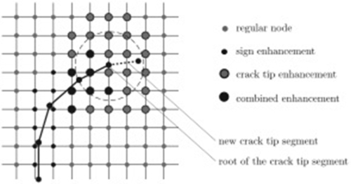
The second additional term in Eq. (4.27) involves a set of branch functions Fl (x) to model the displacement field around the tip of the discontinuity. In LEFM, these functions are chosen based on the well-known asymptotic features of the displacement field at the crack tip. To model a cohesive crack tip, different functions are needed since the stresses at the tip are not singular. An asymptotic analysis of the mechanical fields in a cohesive zone for very large structure has been carried out in Elices et al. (1992), Karihaloo, Xiao, and Liu (2006). The nodes enriched by the branch function form the set K and are shown as gray circles in Fig. 4.24. The support of these nodes contains the cohesive tip. Combined enrichment is obviously possible as shown in Fig. 4.24 (larger black circles).
Introducing the X-FEM approximation (Eq. 4.27) in the displacement variational principle, we obtain the discrete variational statement from which the unknown nodal displacements u i (depending on the number of nodes in the mesh) and the number of additional degrees of freedom to model the presence of the crack (bj and cl k ) can be calculated. The number of additional degrees of freedom depends on the adopted enrichment. The need to use the sign type enhancement where the fracture has opened appears clearly because usual FEM approximations are not discontinuous. As far as the third term is concerned, a node is enhanced by the crack tip enhancement functions if the support of the respective node is located within a circle of radius r e centered in the root of the crack tip segment (see Fig. 4.24). This strategy allows keeping the nodal enrichments unchanged during equilibrium iterations when the global energy criterion is used for crack propagation (Dumstorff and Meschke, 2007). Some authors limited the approximation (Eq. 4.27) to only the first two terms (for instance Mohammadnejad & Khoei, 2013a, 2013b) reducing r e to zero. As a consequence of this choice, the effectiveness of the solution relies on the usual FEM approximation (the first term), requiring a very fine subdivision.
Calculation of stiffness matrices in the discrete displacement variational principle involves integrations over different domains, areas far from the crack, elements cut by the crack without transmission of tractions and an integration over the cohesive zone. The integration over the domain is naturally performed element by element. The other integration requires additional care: for instance in Dumstorff and Meschke (2007), for the element cut by the discontinuity, the integration is performed on each side of the discontinuity separately. For the integration over the cohesive zone, the zone is geometrically represented by a sequence of 1D segments and the integration is thus performed by looping over these segments. Four Gauss points are used on each segment for an accurate integration of the branch functions. Figure 4.25 shows a mesh and a sequence of 1D segments representing the cohesive zone on the mesh.
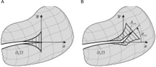
In thermo-hydro-mechanical problems, various enrichment functions can be used to enhance the approximation for pressure and temperature fields, depending on the typical singularities that can be encountered. The displacement field is enriched by the Heaviside and crack tip asymptotic functions, as previously stated. The pressure and temperature fields are enriched by the Heaviside and appropriate asymptotic functions, which are defined based on the analytical solutions of pressure and temperature fields at the vicinity of singularity. The singularity in a discontinuous porous medium can be caused by the thermal and pressure loading in the vicinity of singular points. Since the governing equation of fluid flow in porous media is similar to the heat transfer equation, the treatment of thermal field near the singular points is assumed to be similar to that of the fluid phase. By neglecting the effect of transient terms in the heat transfer equation at the vicinity of singular points and introducing Fourier's law for heat flux, the energy balance Eq. (4.22) can be transformed into ∇2 T = 0 in the absence of heat source, which is also valid near the discontinuity. Boundary conditions must be applied at the discontinuity edges to solve the heat transfer equation. For boundary conditions near the singular points, see e.g., Zamani, Gracie, and Eslami (2010).
A similar procedure can be applied to obtain the pressure distribution in the vicinity of singular points: considering the Darcy equation in steady conditions and disregarding effects of body forces, the continuity equation reduces to ∇2 p = 0. This equation is similar to the steady-state thermal condition and has to be amended by boundary conditions (see Khoei, Moallemi, & Haghighat, 2012). The following branch functions are used in the case of THM problems, respectively for displacement, pressure, and temperature fields:
Fu={Fu1,Fu2,Fu3,Fu4}={√rsinˉθ2,√rcosˉθ2,√rsinˉθ2sinˉθ,√rcosˉθ2sinˉθ}Fp=√rsinˉθ2FT=√rsinˉθ2
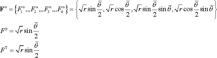
where
ˉθ
![]() is in the range of [− π,π] and is measured from the direction of fracture and r is the local tip coordinate.
is in the range of [− π,π] and is measured from the direction of fracture and r is the local tip coordinate.
To capture the thermo-hydro-mechanical coupling associated with the tractions acting on the fracture and the fluid leak-off from the fracture and heat transfer, the displacement and fluid pressure and temperature fields must satisfy some requirements: a strong discontinuity for the displacement and a weak discontinuity to account for the fluid and temperature flow jump normal to the fracture. Hence, it is required that the fluid pressure and temperature be continuous, while their gradient normal to the fracture be discontinuous.
As observed by Gracie, Wang, and Belytschko (2008), enriched finite element methods (FEMs), such as the X-FEM and the global PUM, are powerful ways of augmenting standard finite element (FE) approximations using known information about the solution of the problem. It is, however, desirable to limit the enrichment to the vicinity of the feature in order to reduce the number of unknowns and improve the conditioning of the system of equations.
Local enrichments have been applied successfully to numerous problems. The method is more accurate than the standard FEM; however, when enrichment is applied to problems with singular fields, the reported results often show the same convergence rate as the standard FEM, which is suboptimal. This degradation of the convergence rate is attributed in part to parasitic terms in the approximation space that arises in the blending elements. A blending element is an element where some but not all of the nodes of the element are enriched. Sukumar, Chopp, Moës, and Belytschko (2001) showed that parasitic terms in the blending elements limit the accuracy of local PUM methods. Several authors proposed strategies for eliminating the parasitic terms. Further, the need of particular care in the integration of elements along the crack has to be recalled.
Bordas, Duflot, and Le (2008) presented an effectivity analysis for crack problems together with a useful error estimator. In mode I problem, when using structured mesh, they concluded that effectivity for various X-FEM enrichment depends on radii of the enriched area. Enriching only the tip element causes an ineffective error indicator nonconvergent to the optimal value. For coarse meshes, higher values of the enrichment radius increase the effectiveness of the indicator. Upon mesh refinement, whatever the enrichment radius, the effectiveness curves meet in the close vicinity of the optimal unity value.
It is interesting to note that the effectivity versus mesh size h curves become closer to the horizontal line e = 1 (optimal value) with increasing enrichment radius. For coarse meshes, large enrichment radii are necessary to obtain an effective indicator. This is expected, as for coarse meshes, near the tip enrichment become dominant over the standard FEM approximation, which in itself is poorly suited to represent the near-tip behavior. As the mesh is refined, the standard FEM part of the approximation becomes more important compared to the enriched part, and the XFEM approximation space tends towards the FEM approximation space. This explains why the use of enrichment for “fine” discretization is ineffective (Bordas & Duflot, 2007), (Duflot & Bordas, 2008).
Few 3D solutions are known for X-FEM, e.g., Gravouil, Moes, and Belytschko (2002), Moës, Sukumar, Chopp, Béchet, and Moës (2008), Bordas and Moran (2006), Bordas, Nguyen, Dunant, Guidoum, and Nguyen-Dang (2007), and Wyart et al. (2007). There are also (in 2D) some papers on multifield problems (for example, piezoelectricity and dynamic crack growth). In 3D, the work of Duflot (2008) on thermomechanics problem is already available, but to our knowledge, no piece of literature addresses in 3D hydraulic fracturing within an X-FEM framework. The evaluation of discretization errors for enriched methods such as the X-FEM deserves particular care. The first studies on error estimation within extended finite element methods were published in the context of the Zhu and Zienkiewicz (1988) recovery-based error estimation techniques. The idea (Bordas & Duflot, 2007) is to smooth the raw X-FEM fields by projecting them upon an intrinsically enriched moving least squares basis (see Nguyen, Rabczuk, Bordas, & Duflot, 2008 for details on such meshless approximations). This idea was shown in Bordas, Rabczuk, and Zi (2008) to provide accurate indication on the error level, even for solutions with large gradients. Slightly later, an extended global recovery technique, based on a projection of the strain field on a global-enhanced space was proposed in Duflot and Bordas (2008).
An extension of the Zienkiewicz–Zhu recovery procedure to enriched (singular and discontinuous) fields, based on a singular-smooth splitting was proposed in Ródenas, González-Estrada, Tarancòn, and Fuenmayor (2008) and bounding estimates given in Ródenas, González-Estrada, Dìez, and Fuenmayor (2010). It was also shown in Barros, Proença, and de Barcellos (2004), Xiao and Karihaloo (2006), and Ródenas et al. (2008), that the use of statically admissible recovery significantly improves the quality of the solution, in particular, that of the crack tip fields. These “admissible” recovered fields can also be constrained to satisfy compatibility. The role of such procedures on the accuracy of the recovered fields in the context of fracture mechanics was discussed recently in González-Estrada et al. (2012). Other works pertaining to error estimation and adaptivity for discontinuous failure were then published in Pannachet, Sluys, and Askes (2009), where various discretization methods and adaptivity schemes are compared. The reader is also referred to the recent work of Prange, Loehnert, and Wriggers (2012), where the authors consider also inelastic material behavior.
Most error estimators in mechanics are in general targeting the error in strain energy. However, the strain energy is usually not a quantity of engineering relevance. Therefore, targeting proper “quantities of interest” or “goals” is gaining popularity, for example, the average stress in a region, the stress intensity factor, the maximum displacement of a structure, and so on. For this, and within an FEM or X-FEM framework, a number of results are available using recovery-based error estimates, González-Estrada et al. (2013), González-Estrada et al. (2014), Panetier, Ladevèze, and Chamoin (2010), Rüter and Stein (2011), Gerasimov, Rüter, and Stein (2012), Lin, Zhuang, You, Wang, and Xu (2012), and Rüter, Gerasimov, and Stein (2013), within the framework of residual-based error estimates. It is not in the scope of this chapter to review the different error estimators available and the interested reader is referred to a didactic review provided in Grätsch and Bathe (2005). Finally, there is only a sparse literature available on a posteriori error estimation for multifield fracture, some of the most noteworthy being Schrefler, Secchi, and Simoni (2006).
4.5 Thick Level Set Model for Localization to Fracture Transition
The thick level set (TLS) model (Bernard, Moës, & Chevaugeon, 2012; Moës, Stolz, Bernard, & Chevaugeon, 2011; Stolz & Moës, 2012) was recently proposed to delocalize local constitutive law suffering from spurious localization. We refer to (Moës, Stolz, & Chevaugeon, 2014) for an up-to-date presentation of the method. It has two major advantages compared to other delocalization methods. The first one is that it acts only when and where needed. That is, the TLS delocalization has no effect on low gradients of internal variables. The second advantage is that the transition from localization to fracture is taken into account in the model. The TLS has been applied so far to damage and fracture of brittle materials only, but is believed promising for other kind of material behaviors, and there is a priori no restriction to combine it with multifield formulations. In order to apply the TLS approach, one must identify in the local constitutive law the variable which may lead to spurious localization. Let us denote this variable as d. We consider in what follows failure of brittle material and d will be the damage variable (the TLS framework is, however, not limited to brittle fracture). The key idea of the TLS is to bound the spatial gradient of this quantity, thus avoiding spurious localization. One imposes
||∇d||≤f(d)onΩ×[0,T],
where Ω and [0, T] are the spatial and time domains, respectively. The choice of the function f will be discussed in what follows. We are interested in models for which localization leads to fracture, i.e., the onset of displacement jumps across boundaries. Finding the zone where d = 1 corresponds to finding the crack location. We face, however, a problem: finding the iso-contour d = 1 of a quantity d that cannot overpass 1 is a tedious operation. This is where the level set ingredient comes into play. Variable d is expressed in terms of a level set ϕ as depicted in Fig. 4.26. This relation introduces a characteristic length l c. Finding the zone where d = 1 is now a well posed problem since the level set ϕ is not strictly limited to l c but may go beyond. Another advantage of the use of the surrogate variable ϕ is that condition (4.29) can be enforced through the two following equations
{d=d(ϕ),||∇ϕ||≤1,

with, f = d′ ![]() d
− 1, d representing a user-defined function of ϕ (Eq. 4.29) and prime symbol representing differentiation with respect to ϕ Eq. (4.30) indicates that ϕ is a distance function in the zone where constraint ||∇ϕ|| = 1 is active. This zone is called nonlocal zone in what follows and is illustrated in Fig. 4.27. We thus fall into the playground of the level set community among which a robust technology has been designed to update distance functions (Sethian, 1999).
d
− 1, d representing a user-defined function of ϕ (Eq. 4.29) and prime symbol representing differentiation with respect to ϕ Eq. (4.30) indicates that ϕ is a distance function in the zone where constraint ||∇ϕ|| = 1 is active. This zone is called nonlocal zone in what follows and is illustrated in Fig. 4.27. We thus fall into the playground of the level set community among which a robust technology has been designed to update distance functions (Sethian, 1999).
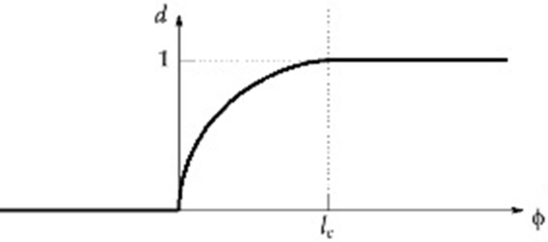
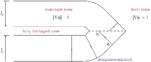
In the nonlocal zone, the evolution of ϕ is nonlocal, indeed
||∇ϕ||=1⇒∇ϕ⋅∇˙ϕ=0.
The rate of ϕ is thus uniform along any segment aligned with ∇ϕ, and the rate of d is given by
˙d=d′(ϕ)˙ϕ
![]() . Consider that the local damage evolution is given by a local relation
˙d=g(Y)
. Consider that the local damage evolution is given by a local relation
˙d=g(Y)
![]() where Y is some local variable. In the nonlocal zone, we replace this local relation by a nonlocal version
where Y is some local variable. In the nonlocal zone, we replace this local relation by a nonlocal version
ˉ˙d=g(ˉY),
where the overline quantities are averages of their local counterpart along segments aligned with ∇ϕ
ˉY(x)=∫ϕbϕaYd′(ϕ)jdϕ∫ϕbϕad′(ϕ)jdϕ,ˉ˙d(x)=∫ϕbϕa˙djdϕ∫ϕbϕajdϕ.
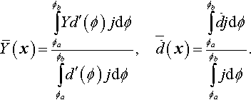
ϕa and ϕb denote the integration bounds on variable ϕ, and j denotes a Jacobian. Following Moës et al. (2014), the integration segments contain the point of coordinate x , are aligned with ∇ϕ and cut through the nonlocal zone characterized by ||∇ϕ|| = 1 (see Fig. 4.27). The above definition of the averaged fields leads to the duality property
∫ϕbϕaY˙djdϕ=∫ϕbϕaˉYˉ˙djdϕ.
As an illustration of the use of the TLS, we consider the plane strain L-shaped panel depicted in Fig. 4.28. A quasi-brittle material is considered and d plays here the role of damage variable. This benchmark, elaborated by Winkler (2001), involves a mixed-mode loading of the crack, and the curved path that is obtained can be confronted to experimental data. The panel is initially crack-free. Figure 4.29 shows that the TLS model is able to predict the development of damage (Fig. 4.29A) followed by crack initiation and growth (Fig. 4.29B). Figure 4.30 shows the load–displacement curve as well as crack path comparison with experimental data. Nodes supported by elements that are cut by the crack are enriched with the X-FEM (Moës et al., 1999).
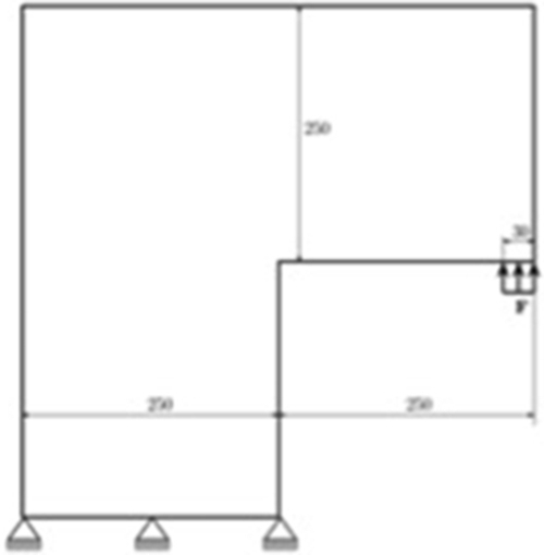
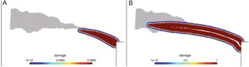
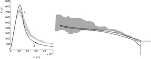
A more detailed presentation of the L-shaped panel example as well as other examples may be found in Bernard et al. (2012). The use of TLS for impact on brittle structure may be found in Moreau, Moës, Picart, and Stainier (2014).
4.6 Phase Field Models
According to Griffith criterion, the crack propagates if the rate of elastic energy decrease per unit surface area of the increment step is equal to the quasi-static critical energy release rate G C. The crack does not move if the elastic energy release rate is less than G C. On the contrary, it is unstable if G C exceeds the critical rate. Griffith found that G C is related to the crack surface energy increase. This statement can neither predict crack initiation nor describe curving and branching cracks: different strategies have been proposed to overcome these shortcomings as we have seen. There is a further one based on phase field models discussed in this section.
Diffusive interface and phase-field models (PFM) (e.g., Bourdin, Francfort, & Marigo, 2008; Francfort & Marigo, 1998; Hakim & Karma, 2009; Kuhn & Müller, 2010) represent the more recent approaches for the above stated goal. In particular, PFM have been proven to be well suited for the description of complex multidimensional, mixed-mode fracture scenarios including dynamic effects and crack branching, see, e.g., Borden, Verhoosel, Scott, Hughes, and Landis (2012) and Miehe, Hofacker, and Welschinger (2010) for more details and references. Instead of modeling the discontinuities explicitly (e.g., as in the X-FEM), the lower dimensional crack surface is approximated by a phase-field function. This introduces a diffusive transition zone (brittle zone or mushy-zone are also common expressions depending on the discipline) between the broken and the unbroken material; see Fig. 4.31. As a consequence there is no need to update or enrich the mesh with proceeding of the fracture.

The modeling of fracture essentially changes if multiphase and heterogeneous porous materials are considered. The problem is due to the inherent coupling of the individual constituents, which is completely disturbed by developing cracks, thereby changing the local physics of the problem.
In the literature, different models for hydraulic fracture simulations can be found, in the respect of a fundamental requirement that there is no need for a preexisting crack to simulate crack initiation. Mikelic, Wheeler, and Wick (2014) propose a phase-field approach for pressure-induced fractures and fluid-filled fractures in porous media based on Biot's equations, which allows the description of different features of crack evolution such as joining and branching. This way of fracture modeling results in a coupled three-field problem (elasticity, phase-field, pressure), which requires a special numerical treatment to obtain stable numerical solutions (see, e.g., Markert, 2013 for details on coupled multi-field problems).
In Markert and Ehlers (2013), the modeling of hydraulic fracturing, as a pressure-driven brittle fracture of fluid-saturated, heterogeneous porous solids, is introduced within a thermodynamically consistent framework using the continuum theory of porous media extended by a diffusive phase-field model. This approach accounts for crack initiation and propagation, the deformation of the solid-matrix and the change of the interstitial fluid flow in the crack and the surrounding porous body. The advantage is that the description of the developing crack path does not require an explicit front tracking, as the kinematics of the crack as diffusive interface is implicitly contained in the extended continuum formulation. However, applying diffusive crack modeling by introducing a phase field as indicator function for the crack adds an additional differential equation to the coupled solid-fluid system. Therefore, also here special attention should be drawn to the spatial and temporal discretization as well as the chosen numerical solution algorithms.
The first step within the phase-field approach is the definition of the potential energy function of a cracked, linear elastic, isotropic body as the sum of the elastic strain energy integrated over the whole body V, and the fracture energy integrated along the crack path Γ c:
F(Γc,ɛ)=∫VˉΨelast(ɛ)︸elasticenergydυ+∫VˉΨcrack(ɛ)︸fractureenergydΓcwith{ɛ:straintensorΓc:crackpath)
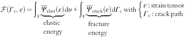
Following this, the phenomenological phase-field variable ϕ is introduced to distinguish between the cracked and the unbroken states of the material, which approximates sharp interfaces (here the crack) by a diffusive transition zone as illustrated in Fig. 4.31.
The potential energy function can be reformulated over the whole body (see, e.g., Francfort & Marigo, 1998) leading to
F[Ψ(ϕ,gradϕ,ɛ)]=∫V[Ψelast(ϕ,ɛ)+Ψcrack(ϕ,gradϕ)]dυ
Herein, the phase-field variable is defined as
ϕ(x,t)∈[0,1]with{ϕ=1:unbrokenϕ=0:cracked)

In this formulation of the potential energy, elastic stress degradation is assumed to occur only under tension, and thus, one distinguishes between the positive (tension) and negative (compression) parts of the elastic energy Ψ elast. In particular, we have
Ψelast(ϕ,ɛ)=ϕ2Ψ+elast(ɛ+)+Ψ−elast(ɛ−)withɛ=ɛ++ɛ−
This split of the elastic energy allows introducing a formulation based on the strain history in order to avoid crack healing in the numerical calculation, see, e.g., Miehe et al. (2010). The fracture energy as a function of the phase field and its gradient can be expressed as
Ψcrack(ϕ,gradϕ)=G4ε(1−ϕ)2+Gε|gradϕ|2{ε:internallengthG:crackresistance)

Having defined the energy functions, the next step is to derive the stress and the phase-field evolution relations. In particular, the stress tensor is defined as the variational derivative of the energy functional with respect to the strain tensor ɛ
σ(ϕ,ɛ)=δFδɛ=ϕ2∂Ψ+elast∂ɛ+∂Ψ−elast∂ɛ
The nonconserved phase-field evolution is derived using the well-known Allen–Cahn diffusion model, which describes the process of phase separation (here crack formation) via a reaction–diffusion equation. Thus, the phase-field evolution reads
∂ϕ(x,t)∂t=−Mδℱδϕ=−M[2ϕΨ+elast−G2є(1−ϕ)−2Gεdivgradϕ]
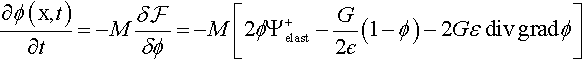
with M being a kinetic parameter related to the interface mobility. It is worth mentioning in this context that improvements could be applied to the Allen–Cahn approach in order to speed-up the computation of the interface movement, for instance, by using the so-called hybrid or Alber–Zhu model (see, e.g., Alber & Markert, 2012). To this end, Eqs. (4.35–4.41) are considered the foundations of the diffusive brittle fracture modeling, which will later be applied to treat hydraulic fracturing of porous media.
In the work of Markert and Ehlers (2013), a biphasic porous body consisting of a solid skeleton φ S saturated by a single interstitial fluid φ F is considered. The binary model is augmented by a phase-field variable ϕ S indicating the degradation of the solid matrix governed by equations similar to the above mentioned. The simplest possibility to account for the crack-induced changes to the pore-fluid flow is to make the permeability dependent on the phase field. It should, however, be noted that this simplification treats the flow in the fluid-filled crack still as porous media flow, which gives space for future improvements, for instance, by using a modified Stokes model.
The treatment within a quasi-static framework leads to a strongly coupled three-field problem, which is formulated in the solid displacement u S, the fluid pressure p, and the phase-field variable ϕ S. The governing balance equations in this case are:
– The mixture momentum balance:
div[σSE(ϕS,ɛS)−pI]=0
with σ E S being the solid effective stress defined comparable to Eq. (4.40), p is the pore-fluid pressure and ɛ S is the linear solid strain tensor (for more details, please refer to, e.g., Markert, Heider, & Ehlers, 2010).
divvS−div[KF(ϕS)gradp]=0
Herein, K F(ϕ S) is the hydraulic conductivity or permeability (isotropic permeability), which depends on the phase-field variable to account for the permeability increase in forming cracks, and v S = (u S)S′ is the solid velocity.
– The phase-field evolution equation (similar to Eq. 4.41)
∂ϕS∂t=−MS[2ϕSΨS+elast−GS2εS(1−ϕ)−2GSεSdivgradϕS]
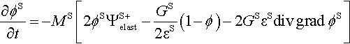
The next step is to solve the strongly coupled differential Eqs. (4.42–4.44) for an initial-boundary-value problem in order to obtain the unknown fields u S, p, and ϕ S. For the numerical solution, the mixed FEM is adopted, which is carried out in two steps: firstly, deriving the weak or variational statements of the governing balance Eqs. (4.42–4.44) and, secondly, using a mixed finite element discretization for the approximate solution of the variational problem. Due to the strong coupling of the governing equations, only special time integration schemes lead to stable numerical solutions (see, e.g., Markert et al., 2010 and Markert, 2013 for a detailed discussion on coupled problems).
In order to give a qualitative benchmark example, the proposed diffusive porous media fracture model is applied to a 2D test case, where the fracture-induced changes to the fluid percolation are investigated. In particular, a rectangular porous material with moderate permeability and included low-permeability barriers is subjected to a pressure gradient from bottom-left high-pressure (red (gray in print version)) inflow to top-right low-pressure (blue (dark gray in print version)) outflow (Fig. 4.32, left). The double-notched porous medium is then set under tension inducing typical mode 1 fracture. The changes to the permeability (from low/blue to high/red) and the flow path are observed while the cracks propagate. As expected, the model predicts the permeability increase in the degraded or cracked material, thereby strongly affecting the pore-fluid flow regime (see Fig. 4.32, right). From the streamlines indicating the flow path, it is apparent that the nature of the flow changes completely from the unbroken porous matrix to the finitely opened cracks.
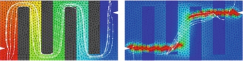
The major advantages of using phase-field modeling for crack propagation are fourfold. First, it is a fixed-mesh approach in which remeshing is avoided. Second, the model is purely based on energy minimization and therefore, crack nucleation, propagation, and the path are automatically determined (avoiding calculation of additional components such as stress intensity factors). Third, multiple joining and branching of cracks do not require any additional techniques. Consequently, phase field modeling allows simple handling of large and complex fracture networks. Fourth, crack growth in heterogeneous media does not require any modification in the framework. Quantities of interest such as the crack opening displacement (the aperture) can be recovered with the help of the phase-field function (Wheeler, Wick, & Wollner, 2014).
4.7 Discrete Crack with Adaptive Remeshing
This method is discussed in some detail because together with the lattice and fuse model (Milanese, 2014; Salerno, Maloney, & Robbins, 2012 and Zapperi, Vespignani, & Stanley, 1997) is able to capture avalanche-type behavior of the fracturing process, see Sections 6.4 and 7.
The method solves directly the governing equations of Section 3 and requires continuous remeshing of the domain because the topology changes with advancing fracture. In our opinion, this method appears as the most suitable one to represent the full physics in the fracturing domain in multifield problems. No smearing of properties over some domain such as an element or diffuse interfaces is required. We describe now the necessary ingredients. To account for the continuous changes of topology of the domain Ω and its boundary with the evolution of the fracture, an adaptive remeshing technique is used based on an a posteriori error analysis of a previously obtained solution. All the governing equations are simultaneously solved, even though staggered solutions may also be devised (Turska & Schrefler, 1993). The fracture path, the position of the process zone and the cohesive forces are unknown, together with the pressure and temperature fields. The efficiency of the overall procedure is based on the efficiency of the discretization in space, which is shortly summarized in the following. Owing that crack propagation is analyzed in slightly different way depending on the dimension of the domain (2D or 3D), the same distinction is made for the mesh generation and fracture tip advancement.
4.7.1 2D Mesh Generation
An improved implementation of 2D Delaunay triangulation is used leading to unstructured planar meshes defined in simply or multiply connected regions of any arbitrary shape (Secchi & Simoni, 2003). The algorithms belonging to the Delaunay–Voronoi class offer the advantage of efficiency together with a sound mathematical basis. The computational cost of the used algorithm is ranging from O(N1.5) to O(N logN), but, avoiding some not strictly necessary quality checks, can be reduced to almost O(N). Further, it pursues flexibility, reduction of user intervention, quality of the mesh, and computational efficiency, independently of the complexity of the domain.
To obtain high computational performances, the capabilities of an object-oriented language are exploited and a modified edge-based data structure is built for storing mesh topology information and handling meshing operations. A series of newly defined primitives and higher level topological operators perform the necessary operations, speed up the procedure and limit memory requirements. The defined primitives and operators, together with an edge-based data structure almost completely avoid the need of computational loops in meshing operations, resulting in a highly efficient generation procedure.
The only user intervention consists in a schematic description of the boundary of the domain (polygonal contours and/or analytical curves) and the location of singularities, for instance sources or sinks. Each geometrical entity is associated with a function controlling the spacing of the nodes to be generated (spacing function). Automatic refinements deal with a priori node grading along the boundaries and with the management of mesh and geometric singularities. Once new nodes are generated, the spacing function is interpolated from the existing nodes. The final discretization depends only on the initial description of the boundary (assigned nodes and spacing function) and there is absolutely no guarantee that with arbitrary input data a good quality mesh can be obtained. To improve this situation, a special algorithm is defined which corrects the boundary description when highly distorted elements originate from the assigned data, running from the initial steps of the generation:
– the nodes are inserted beginning with those at the boundary. The topological entities defining the boundary handle the node distribution by accounting for the spacing function at the end points. For closed contours, the spacing function is assigned a constant value. The boundary entities recognize the regions connected to them by means of information present in their structure, not through searches in special lists and without any orientation rules, and require the region/s topological entities to locate the new common node. Each region then handles separately the generation of triangles and contours, and conformity checks, following the usual Bowyer (1981) Watson (1981) algorithm;
– consistency checks along each interface are made. Once the node location phase has been accomplished, there is no guarantee that the interface boundary is represented by the triangulation edges. The geometric consistency is controlled and, if necessary, can be reached by inserting new nodes as in the basic procedure. In the presence of nonhomogeneities, the region entities indicate the existence of the anomaly and require the boundary to locate a new node in a fixed position. The boundary entity continues with the insertion of the node, but informs all other regions linked to it of this operation. This procedure is repeated until the consistency of all boundaries is obtained.
From the computational point of view and to improve the efficiency of the generator, all the required meshing operations are performed by special Euler operators which exploit the information contained in the data structure representing the fundamental entities, Vertices, Edges, and Faces. Owing to the data structure used, the existence of conditional loops is almost completely avoided, this resulting in a highly efficient computer code.
Particularly interesting for nonhomogeneous materials and fracture problems are some capabilities of the generator such as the node grading along the boundaries, management of mesh and geometric singularities and a strict preservation of the shape of the singularity and/or the interface. In the case of nonhomogeneous materials, each homogeneous region is meshed independently from the others, using completely independent spacing function values with the unique requirement of assuming the same value along the interfaces for the neighboring zones to guarantee mesh consistency and approximation continuity. Further, it is necessary that the triangulation completely represents the boundary of each region and the complete domain. It should be remembered that Delaunay triangulation is a unique geometric construction for an assigned set of points; hence it does not guarantee the consistency of a generic contour defined through a subset of points of the initial set.
The algorithm used produces the initial mesh with element dimensions controlled by a user-defined spacing function and automatically accounts for geometrical domain singularities, improving mesh quality, and curved boundary representation. With proceeding the fracturing process the domain is first updated, accounting for fracture movements, then is triangulated by controlling the dimension of the elements using the a posteriori error measure proposed by Zhu and Zienkiewicz (1988). A quadrilateral mesh, sometimes preferred in fracture mechanics, can also be obtained, preserving mesh quality control. In both cases, linear approximation of the field variables is used. To reduce computation time, the successive refinement/derefinement operations can be limited to suitable subdomains containing the singularities zones. The dimensions of these areas and local density of discretization can be decided on the basis of the solution at the previous steps.
4.7.2 Fracture Nucleation and Propagation
Evolution of discrete fracture results in a continuous change in the topology of the domain together with the updating of boundary conditions. Whereas changes in topology are dealt with by the remeshing of the domain, mechanical, and kinematical boundary conditions are treated by means of the Lagrange multipliers technique.
In order to model the open crack and process zone, finite elements are used that present only the cohesive forces for the solid phase and account for the complete behavior for the fluid phase. As a consequence, these elements allow for a straightforward integration of Eq. (4.15) in the fracture domain, without requiring special treatment of the continuity equation along the open fractures. Finite elements located along the fracture path can be viewed as special nonlinear contact elements, capable of representing mixed mode fracture behavior, as well as integrating the fluid continuity equation along the crack path.
Let us consider a nonhomogeneous 2D domain under plane strain or stress assumptions. In a generic solution step, once the displacement and pressure fields have been obtained, strain and stress fields are calculated. The latter, given that linear approximation of the field variables is used, are constant within each element. Nodal values of stresses are calculated by applying a smoothing procedure only to elements of the same material. Stress discontinuities can therefore be present only at nodes belonging to an interface, whereas the stress field is continuous within each homogeneous region. Given that unstructured meshes are used, each node can be shared in general by n elements with nm different material properties. The topological entity node is required to handle nm stress and strain tensors together with fracture nucleation/propagation. This means that all cracks required by the stress field can be present at the same time.
Even in the presence of nonhomogeneous materials, when the fracture moves within a generic homogeneous subregion it is assumed that nucleation and propagation take place according to the model of Section 2.2. When the fracture path approaches an interface between two different materials the direction of propagation can be different from the previous case. It is chosen to maximize the energy fracture release.
The evolution of the fracture paths involves continuous transformation of the solid phase domain. This is handled by changing the finite element mesh at each step of the solution. The computational procedure to find the point of crack formation consists in finding the node Ni with the highest principal positive stress. When this exceeds the limiting value of the material, a new crack is created or an existing one moves its tip. If a new crack nucleates, the following cases are possible:
– node Ni is inside the domain. The existing node is eliminated and four new nodes are inserted together with four new edges (Fig. 4.33A). The trial advancing step is defined a priori. If the fracture progress brings the tip N n + 2 or N n + 4 into a circular neighborhood of radius d zip of an existing node, the tip is repositioned in correspondence to the existing node. The distance d′ between the two lips of the fracture is initially assumed somewhat greater than d zip to avoid the elimination of one of the new nodes N n + 1 or N n + 3. The assumptions introduced for the longitudinal and transversal dimensions of the fracture are mere operative choices and do not influence the evolution of the phenomenon, which is governed by the balance equations only;
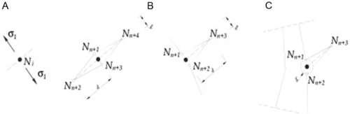
– node Ni belongs to the boundary (external or interface). Once the existing node is eliminated, three new nodes and two edges are located (Fig. 4.33B). The propagation direction is determined so that the formation of a convex boundary is guaranteed;
– node Ni belongs to a border of an existing fracture external to the process zone (Fig. 4.33C). The same operational choices as in the previous case are adopted;
– node Ni belongs to the process zone (Fig. 4.33C). The procedure operates in the same way as in the previous cases, except for the application of the cohesive tractions along the existing fracture and the one branching out from it.
If an existing crack is propagating, the following cases are possible:
– the fracture is propagating inside a homogeneous region. The advancing direction is assumed in order to guarantee the concavity of the new boundary. If alternative possibilities are present, the advancing direction is chosen such that it guarantees the maximum fracture energy dissipation. The crack advances at a step of length d, which is obtained by splitting the node in the previous position of the tip (nodes N n + 1 and N n + 2 are created) and the new node N n + 3 is inserted at distance d (Fig. 4.34A);
– the fracture advancement of a predetermined quantity d results in crossing an interface or locating a new node external to the geometric domain ΓM (Fig. 4.34B). The step length is reduced to d*, this being the distance of node Ni from the interface or boundary along the direction of propagation. The geometric entities describing ΓM are then rebuilt, due to the fact that they have been modified by the insertion of the new node. This step may result in the formation of new regions and new boundaries (Fig. 4.35);
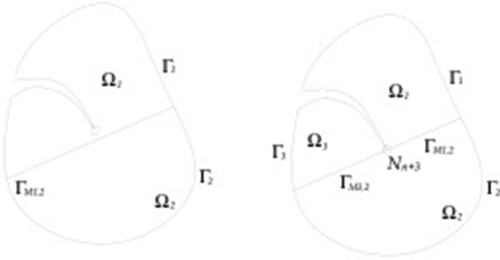
– node Ni belongs to the interface. The fracture may propagate inside one of the adjacent regions or along their interface. Of the different propagation possibilities, the one involving the maximum fracture energy dissipation is chosen. If the first case takes place, because of the continuity of the displacement field and the assumed isotropy of the components, the principal stress directions are coincident in the different materials. Hence, the direction of the fracture propagation can be calculated by using the same procedure as in the previous cases. Once the new tip node has been determined, cohesive tractions are calculated by means of the constitutive relationships of the material of the region containing the new node. When the angle between one of the new edges and the interface is somewhat smaller than a user prefixed value, the new node is projected on the interface ΓM and the procedure operates as in the case of crack propagation along the interface. In the latter case, tangential forces are usually present between the fracture lips. The exchanged tractions are determined on the basis of mixed mode fracture propagation using Eqs. (4.8) and (4.9).
As seen, the advancement of a fracture creates new nodes: in 2D the resulting new elements for the filler (elements in the open crack) at the front are triangles. It is important to point out that with the chosen algorithm at each time station tn, j successive tip (front) advancements are possible until the Rankine criterion is satisfied (Fig. 4.36). Their number in general depends on the chosen time step increment Δt, the adopted crack length increment Δs, and the variation of the applied loads.
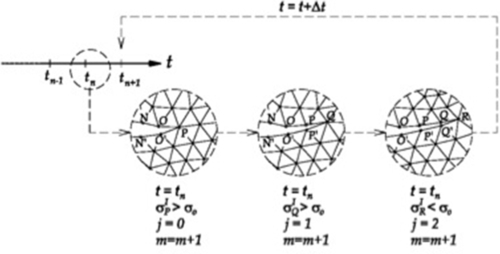
The required continuous remeshing involves transfer of nodal vectors from the old to the continuously updated mesh by a suitable operator v m(Ω m + 1) = ℵ(v m(Ω m)). For momentum and energy conservation, the solution is repeated with the quantities of mesh m but recalculated on the new mesh m + 1 before advancing the crack tip (Secchi, Simoni, & Schrefler, 2007). This will be explained in Section 5.
When geometric or mesh singularities are located near the boundary, generating high gradients of the spacing requirements (Fig. 4.37, top), the algorithm updates the grading along the boundary and improves the geometric description, maintaining the topology of the domain (solution independent mesh improvements). The same procedure, which controls the grading along the boundary, allows for quality control of the complete resulting grid. In this sense, the subdivisions produced, although not optimized as finite element meshes, are certainly very appropriate from the geometric point of view and represent an optimal starting point for adaptive algorithms in numerical solutions. Good meshes are hence obtained by means of a unique process, without any correction phase, even in the presence of very irregular boundaries and geometric constraints. As an example, Fig. 4.37, bottom, represents the mesh improvements related to the presence of a material discontinuity line crossing the domain.
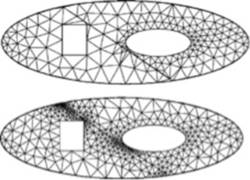
4.7.3 Space-Refinement Strategy
In the frame of h-refinement method in space, a total or partial remeshing technique is adopted. For all variables, linear approximation of the fields is used. This may lead to possible locking for small permeability. This choice has been, however, preferred to overcome the problems of transferring information between different meshes and is supported by the fact that in our numerical experiments with the usual values of permeability locking has never been experienced.
To reduce computation time, the successive refinement/derefinement operations can be limited to suitable subdomains containing the singularity zones. These subdomains can also coincide with the areas where different mathematical models apply. The dimensions of these areas and local density of discretization can be decided on the basis of the solution at the previous steps. The link between the refinement and the mesh generator is the spacing function, which is point-wise updated according to the a posteriori calculated error. The spacing function and the ensuing node distribution are then regularized by interpolation when the new nodes are inserted. In this way, the resulting discretization always presents a smooth distribution of element dimensions (Secchi and Simoni, 2003); further unstructured and nondirectional meshes are obtained.
The general scheme of the refinement procedure is presented in Fig. 4.38. It is important to remark that the first step is performed by the mesh generator using the multiconstrained algorithm previously described, when a geometrical singularity is detected. Then the Zhu and Zienkiewicz (1988) technique is adopted, which relies on an a posteriori recovery-based error estimator. In the original proposal, this approach is applied to stress field that is to the flux term of the displacements. The same procedure is here applied to fluxes (hydraulic and thermal), which depend on spatial first derivatives of the pertinent field variables. The error energy norm is calculated locally over a patch formed by the elements, usually six, surrounding each node of the actual mesh. This error is related to the maximum permissible error. A weighting parameter is hence obtained by which the spacing function in the central node of each patch is multiplied. Note that in the used mesh generator the spacing function is defined point wise, whereas in standard adaptive procedures the generic element is directly handled. The used approach has the advantage of producing more regular and graded meshes. All field variables are involved in the adaptive procedure. Even though it is possible to use different discretizations for different fields, in our applications the same mesh for all fields is always employed. As a consequence, in the case of conflicting refinements indicators the stricter one is applied. We have observed that the stricter requirements come generally from the solid field.
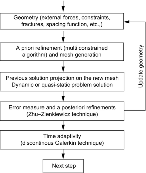
In this way, several purposes are attained at the same time: approximation is enriched where needed by the singularities of each field (i.e., the computational cost is limited), the good conditioning of the system is maintained, no blending elements are present, and the optimality of the overall solution procedure is preserved. Hence, in spite of the cost of the remeshing procedure, the obtained advantages are remarkable.
Zhou and Molinari (2004) suggest three basic rules for a correct space discretization: (i) small mesh size, (ii) mesh size as uniform as possible, (iii) random orientation of elements in order to avoid preferred directions.
The adopted strategy guarantees all these requirements: it is in fact based on a Delaunay tessellation, hence it produces random distribution of elements, without using highly distorted elements. For the process zone, we locate at the tip of the fracture a point element source with strength controlled by the user, that is by using the mechanical properties of the medium, or by the discretization error; uniformity of the mesh in the area surrounding the crack is assured by the interpolation of the spacing function and by ad hoc operators of the remeshing procedure.
By operating in the frame of remeshing, in the used procedure we obtain for instance for a four point bending test the discretizations shown in Fig. 4.39. A typical mesh for the similar three point bending test using X-FEM is shown in Fig. 4.40 (e.g., Moës and Belytschko, 2002).
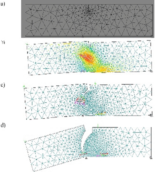
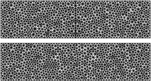
The comparison of the two discretizations of Figs. 4.39 and 4.40 suggests that by refinement strategy a more rational element distribution is obtained with refining limited to the areas with higher gradients and optimal mesh grading is at the same time obtained, which guarantee the correctness of the solution. Further the procedure is fully automatic and only essential domain description is needed, limiting the analyst's intervention and the initial guess of the solution. Eventually, as can be seen in Fig. 4.39, the obtained distributions of cohesive forces are very regular.
Even though the above presented mesh adaptivity algorithm is always active, for relative energy norm percentage errors typically adopted in engineering problems we have found that the most pressing requirements are those of a proper representation of field singularities, such as the process zone where cohesive tractions can take place. This will be addressed next.
Although there is already a large body of literature reporting the successful use of cohesive zone models in analyzing fracture problems in various context (single, multiphase, e.g., Elices et al., 2002), an inconvenient fact less often mentioned in cohesive zone model analyses is that, the softening part of traction–separation laws that governs the damaging process requires a very refined mesh at the crack tip region: characteristic element size has to be less than 1/3–1/5 of the cohesive zone size to achieve reasonable numerical accuracy and stability, see e.g., Carpinteri and Colombo (1989), Moës and Belytschko (2002), Do, Liu, Yang, and Su (2013). Given the fact that the cohesive zone size is typically much smaller than the structural dimensions, this requirement is prohibitively expensive for fracture analysis at the structural level when the fracture path is unknown and a fixed mesh is used. The strict requirement for mesh size led some researchers to use reduced cohesive strength to artificially increase the cohesive zone length, hence to achieve numerical stability, see, e.g., Camanho, Davila, and de Moura (2003), Turon, Camanho, and Costa (2006). However, it should be cautioned that such numerical treatments result in incorrect crack-tip stress fields and should be used only when the existing crack length is much larger than the cohesive zone length. This aspect is strongly emphasized in coupled problems. For instance, in hydraulic fracturing, the correct representation of the crack involves at the same time water pressure within it and, in turn, forces applied to the fracture lips, which influence crack evolution. This aspect will be further addressed below.
It is instructive to analyze the results of the simulation of the three point bending test in a concrete beam problem carried out with cohesive elements which share the nodes with abutting elements (Do et al., 2013). This is a one-field problem (the mechanical one), which is widely present in fracture literature. It has been generally established that a cohesive element with linear displacement distribution along the bonding edge is preferred. This is because a linear cohesive element guarantees a monotonic change of crack displacements within the element as it evolves toward failure, while a high-order element with midnodes may result in serious contact at the midnode pairs even if the crack displacements at the corner nodes undergo monotonic changes (Camanho et al., 2003, and Schellekens & de Borst, 1996). Contact at node pairs is a major source for numerical instability as has been clearly demonstrated in Qiao, Chen, Yang, and Lua (2011). In order to reduce the computational costs when using linear elements, for which dimensional requirements are stricter, improved integration schemes of the Gauss and Newton–Cotes type are introduced for the process zone. Being h the height of the beam and le the mesh size, Fig. 4.41 clearly shows that with fine discretization (h/le = 20), the mechanical behavior is correctly represented by all the integration methods, whereas for coarse mesh (h/le = 2) even the more accurate integration schemes are not able to represent the correct solution (assumed as the one obtained by Moës & Belytschko, 2002 using X-FEM).
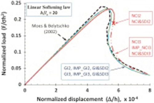
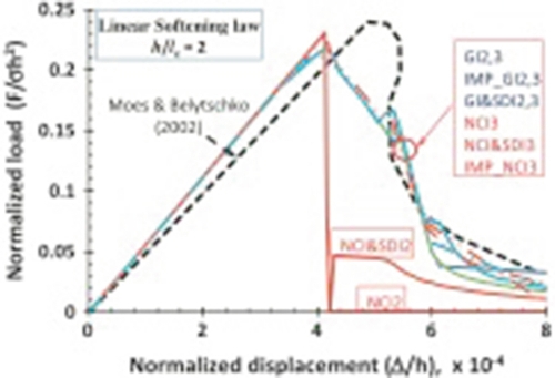
Further, Fig. 4.42 presents the results obtained with improving the discretization from h/le = 2–10 and demonstrates the substantial equivalence of the linear and bilinear softening laws. The conclusion of this experiment is that it is not sufficient improving the integration rule along the cohesive zone, but it is necessary to discretize sufficiently this area and in the presence of an adaptive technique, to account for this in the refinement procedure.
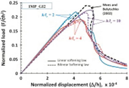
A second stage of the refinement and adaptivity procedure in fact deals with the process zone, according to the proposal of Falk, Needleman, and Rice (2001), and is as follows (Schrefler et al., 2006): the length of the process zone is a priori estimated for the assigned material properties and geometry similar to the case at hand. Once this length is obtained, the analyst can choose the number of elements to represent it (element threshold number). This allows constructing a goal-oriented refinement (Fig. 4.43), to control the trial advancing step Δs and, as a consequence, the velocity of the crack tip.
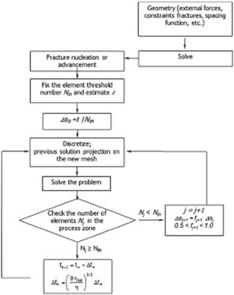
In multifield problems, different singularities may arise within the domain, for instance in hydraulic fracturing a region of reduced pressure develops between the fluid front and the fracture tip, i.e., the fluid lag. This has unknown, but small dimensions (Garagash & Detournay, 2000) and strongly influences fracture propagation (Advani et al., 1997). In an LEFM context, it has been demonstrated that a finite lag is required to ensure coherence of the mathematical solution. Otherwise, a combination of the water mass balance equation and the singular solution for the solid, which is r 0.5 for the stress field, implies a logarithmic singularity for the pressure. This is not only mathematically inconsistent with the eigensolution of the problem, but also with the physical assumption of limited fluid pressure, usually zero (Carter et al., 2000). The tip cavity is in fact filled with evaporated fracturing fluid under constant pressure, negligibly small compared with the stress field far from the fracture. Whereas the crack tip moves at a speed dependent on the mechanical characteristics of the medium, the fluid within the fracture moves depending on permeability defined by the Poiseuille law. The lag dimensions hence change in time. This is true also in presence of cohesive forces.
In the used approach, no simplifying assumption is required for fluid lag or the pressure value within it. All information is obtained through the solution of the governing equations, which combine cohesive mechanics behavior and heat and fluid transport. An important consequence must be drawn regarding the numerical approximation of the field variables. The behavior exhibited by the solid and fluid fields is different. The cohesive effects in fact smooth the stress field, which, however, presents local concentrations, whereas the fluid pressure is more regular because of the limited pressure value at crack tip. As a consequence, it is not advisable to use special fracture elements and the same approximation for the two-field is a reasonable solution. This, however, is a very demanding requirement and the above presented mesh generator together with the a posteriori error refinement has proved to be very effective in the applications. The goal-oriented procedure can be easily extended to correctly represent the fluid field in the process zone and the fluid lag. The only need is to estimate the length of the fluid lag on the base of the previous numerical solution and the element threshold number to be satisfied over the process zone.
4.7.4 3D Problems
The 3D discrete fracture approach, which uses remeshing in an unstructured mesh together with automatic mesh refinement is presented in Secchi and Schrefler (2012). By modifying the data structure which constitutes the base of the 2D discretization technique presented in Section 4.7.1, a numerical procedure for managing generic tetrahedral elements has been obtained in the case of non-manifold surfaces. This new structure preserves the edge algebra and all mathematical and topological properties as well as efficiency in handling the adjacency of the Face Edge. In addition, it has been equipped with some new primitives directed to managing all the different meshing operations in a 3D context.
Geometrical information is preserved; hence the queries are performed in a limited time, almost independently of the number of elements in the list. For this reason, the topological structure also allows for a rapid execution of operations such as swapping of edges, mesh quality control and similar tasks, in particular it is suitable for representing spatial surfaces and solids by means of triangles or polygonal surfaces of higher complexity and to deal with tetrahedral subdivisions. The usual topological transformations (translations, rotations, scaling) as well as more complex operations in space (such as sectioning of solids and their spatial visualization) are also possible by adding a small amount of extra data.
In the resulting procedure, the fracture is assumed to follow the face of the elements around the fracture tip which is closest to the normal direction of the maximum principal stress at the fracture tip. Note that as compared to a 2D situation the fracture tip becomes here a curve in space (front). Along the formed crack faces and in the process zone, boundary conditions are the direct result of the field equations. The adopted remeshing technique accounts for all these changes.
With proceeding of the solution, at each time station tn , again all the necessary spatial refinements are made, i.e., j successive front advancements are possible within the same time step. If a new node is created at the fracture advancement front the resulting elements for the filler (elements inside the fracture) are tetrahedral. If an internal node along the process zone advances, a new wedge element results in the filler.
Except for these aspects, 3D procedure presents the same advantages and problems as the 2D formulation, as will be discussed in Sections 6.3 and 7.