Point and Interval Types Revisited
This chapter discusses a number of miscellaneous issues arising from the fundamental interval type notion and the related point type notion. First, it considers the possibility of supporting several distinct successor functions for “the same” point type; in particular, it shows how the concept of type inheritance can be used to support that possibility. It also considers the pragmatically important special case of intervals defined over points of type NUMERIC(p,q) for some precision p and scale factor q. This latter discussion leads to the need to extend the type inheritance concepts already discussed to deal with multiple inheritance. The chapter also revisits the notion of granularity from Chapter 4 and considers how that notion relates to the more familiar notion of scale.
Keywords
type inheritance; successor function; multiple inheritance; precision; scale; granularity
Second thoughts are best.
—late 16th century proverb
It’s time to take care of some unfinished business. In Chapter 6, we said every interval type involves an underlying point type, and a point type is essentially just a type that has a successor function. Here’s the pertinent text from that chapter (irrelevant material omitted):
A given type T is usable as a point type if all of the following are defined for it:
■ A total ordering, according to which the operator “>“ (greater than) is defined for every pair of values v1 and v2 of type T, such that if v1 and v2 are distinct, exactly one of the expressions v1 > v2 and v2 > v1 returns TRUE and the other returns FALSE
■ Niladic first and last operators, which return the smallest and largest value of type T, respectively, according to the aforementioned ordering
■ Monadic next and prior operators, which return the successor (if it exists) and predecessor (if it exists), respectively, of any given value of type T according to the aforementioned ordering
However, it turns out that there’s a lot more to be said on the topic of point types in general (and therefore on the associated topic of interval types as well); hence the present chapter. Unfortunately, it also turns out that a great deal of groundwork needs to be laid, and a large number of implications and ramifications need to be explored, before we can really get to the substance of some of the issues. Thus, if you find it seems to be taking a long time for the true significance of the chapter to emerge, we just have to ask you to be patient; that true significance will—we hope—emerge eventually.
Ordered vs. Ordinal
Our first point is this: As you might have noticed, that definition from Chapter 6 gives a list of conditions that are certainly sufficient for a type T to be usable as a point type—but are they all necessary? In what follows, we’ll show (eventually) that the answer to this question is no. But first things first. We begin by drawing a distinction between ordered and ordinal types:
Definition: An ordered type is a type for which a total ordering is defined. In other words, an ordered type is a type T such that the expression v1 > v2 is defined for all pairs of values v1 and v2 of type T, returning TRUE if and only if v1 follows v2 with respect to the applicable ordering.
Definition: An ordinal type is an ordered type for which certain additional operators are defined: first, last, next, prior, and possibly others.
■ Type INTEGER is an ordinal type. In fact, we can say more specifically that any given type is an ordinal type if and only if it’s isomorphic to type INTEGER.
■ By contrast, type RATIONAL (“rational numbers”) is an ordered type but not an ordinal one, because if p/q is a rational number, then—in mathematics at least, if not in computer arithmetic—there’s no rational number that can be said to be “next” in numerical order, immediately following p/q.1
Given these definitions, we can now say that all of the types, apart from interval types, that we’ll be discussing in this chapter—until further notice, at any rate—will be ordinal types specifically. For simplicity, therefore, from this point forward we’ll take the unqualified term type to mean an ordinal type specifically, where it makes any difference (unless the context demands otherwise, of course).
Now, in Chapter 6, we made a crucial assumption: to be specific, we assumed the successor function for a given point type was unique (in other words, if T is a point type, then T has exactly one successor function). However, we also said this assumption was a very strong one, and we gave the example of a type, “calendar dates,” for which we might want to consider two distinct successor functions, “next day” and “next year.” (In fact, we might want to consider many different successor functions for this type: “next day,” “next business day,” “next week,” “next month,” “next year,” “next century,” and so on.) And we promised to come back to this issue later. Now it’s time to do so.2
It turns out that the key to the problem we’re trying to solve is the notion of type inheritance. We therefore begin with a section—unfortunately but inevitably a little on the lengthy side—describing the salient features of that concept.
Type Inheritance
A robust, rigorous, and formal model of type inheritance (inheritance for short) is presented in references [51-52], and it’s that model we’ll be following here. Note: We mention this point right away because several different approaches to inheritance are described in the literature (and implemented, in some cases, in commercial products and languages), yet we find at least some of those approaches to be logically questionable. This isn’t the place to get into details; please just be aware that the approach described in the present book differs in certain important respects from approaches described elsewhere in the literature.
Consider the type “calendar dates” once again. In contrast to earlier chapters, assume this type is not built in (this assumption allows us to illustrate a number of ideas explicitly that might otherwise have to be implicit). Also, let’s agree to call this type not DATE but DDATE, in order to emphasize the fact that it denotes dates that are accurate to the day. Of course, DDATE is an ordinal type; its values are ordered chronologically, and the successor function is basically “next day,” or in other words just “add one day.” We’ll give a definition for this operator (also for the associated first, last, next, and prior operators) in the next section, “Point Types Revisited,” but here’s a definition for the type as such:
TYPE DDATE POSSREP DPRI { DI INTEGER CONSTRAINT DI ≥ 1 AND DI ≤ N } ;■ Type DDATE has a possible representation called DPRI (“DDATE possible representation as integers”) that says that any given DDATE value can possibly be represented by a positive integer called DI.
■ The CONSTRAINT portion of the POSSREP specification constrains type DDATE to be such that values of DI must lie in the range [1:N], where N is some large integer (we leave the actual value of N unspecified here to avoid irrelevancies).
Please refer to Chapter 1 if you need to refresh your memory regarding either possible representations (possreps for short) in general or type constraints in particular.
Now, we saw in Chapter 1 that every type requires (a) an equals operator and (b) for each declared possrep, a selector operator and a set of THE_ operators (actually just one THE_ operator, in the case at hand). Here are definitions of those operators for type DDATE. Note: The implementation code for the equals operator, at least, can and probably should be provided automatically by the system. We show it here explicitly for pedagogic reasons.
OPERATOR DPRI ( DI INTEGER ) RETURNS DDATE ;
/* code to return the DDATE value corresponding */
/* to the given integer DI */
END OPERATOR ;
OPERATOR THE_DI ( DD DDATE ) RETURNS INTEGER ;
/* code to return the integer corresponding */
/* to the given DDATE value DD */
END OPERATOR ;
OPERATOR “=” ( DD1 DDATE , DD2 DDATE ) RETURNS BOOLEAN ;
RETURN ( THE_DI ( DD1 ) = THE_DI ( DD2 ) ) ;
END OPERATOR ;
The selector operator DPRI allows the user to specify, or select, a required DDATE value by providing the appropriate positive integer. (You can think of it as an operator for converting a positive integer to a DDATE value, if you like.) For example, the DPRI invocation
DPRI ( 59263 )
returns whatever DDATE value—i.e., whatever date in the calendar, accurate to the day—happens to be 59,263rd in the overall ordering of such values. However, what’s clearly missing here is a more user friendly way of specifying such DDATE values. So let’s extend the type definition to add a second possrep, thus:
TYPE DDATE POSSREP DPRI { DI INTEGER CONSTRAINT DI ≥ 1 AND DI ≤ N } POSSREP DPRC { DC CHAR CONSTRAINT …………………… } ;The CONSTRAINT specification for possrep DPRC (details of which are omitted here for simplicity) constitutes another constraint on values of type DDATE; it consists of a probably rather complicated expression that constrains such values to be such that they can possibly be represented by—let’s assume—character strings of the form yyyy/mm/dd, where yyyy is an unsigned positive integer in the range [0001:9999],3 mm is an unsigned positive integer in the range [01:12], dd is an unsigned positive integer in the range [01:31], and the overall yyyy/mm/dd string abides by the usual calendar rules. Of course, every value of type DDATE has both a DPRI representation and a DPRC representation, a fact that implies among other things that every DPRI value must be representable as a DPRC value and vice versa.
We also need a selector and a THE_ operator corresponding to the DPRC possrep:
OPERATOR DPRC ( DC CHAR ) RETURNS DDATE ;
/* code to return the DDATE value corresponding */
/* to the given yyyy/mm/dd string DC */
END OPERATOR ;
OPERATOR THE_DC ( DD DDATE ) RETURNS CHAR ;
/* code to return the yyyy/mm/dd string corresponding */
/* to the given DDATE value DD */
END OPERATOR ;
Now the user can write, e.g.,
DPRC ( '2013/07/20' )
to specify a certain date—July 20th, 2013, in the example—and
THE_DC ( d )
to obtain the character string representation of a given DDATE value d.
Note: In practice, we would surely want to define numerous additional operators in connection with type DDATE: one to return the year corresponding to a given DDATE value, another to return the month, another to return the year and month in the form of a yyyy/mm string, another to return the day of the week, various arithmetic operators (e.g., to return the date n days before or after a specified date), and many others. We omit detailed discussion of such operators here, since they’re irrelevant to our main purpose.
To get back to that main purpose, then: We can use type DDATE to illustrate the concept of type inheritance by observing that sometimes we’re not interested in dates that are accurate all the way to the day. For example, sometimes accuracy to the month is all that’s required—the day within the month is irrelevant. Equivalently, we might say that, for certain purposes, we’re interested only in those values of type DDATE that happen to correspond to (let’s agree) the first of the month—just as, e.g., when we count in tens, we’re interested only in those numbers that happen to correspond to the first of each successive sequence of ten integers (10, 20, 30, etc.).
Now, if we’re interested only in a subset of the values that make up some type T, then by definition we’re dealing with a subtype—call it T'—of type T. In a geometric system, for example, we might have two types called RECTANGLE and SQUARE, with the obvious semantics; and since every square is certainly a rectangle, albeit a special case, we can say that (a) every value of type SQUARE is also a value of type RECTANGLE, and hence that (b) type SQUARE is a subtype of type RECTANGLE. Here’s a definition:
Definition: Type T' is a subtype of type T if and only if every value of type T' is also a value of type T (i.e., the set of values of type T' is a subset of the set of values of type T).
■ Every type is a subtype of itself (because every set is a subset of itself).
■ If T' is a subtype of T and T” is a subtype of T', then T” is a subtype of T.
■ If T' is a subtype of T and there’s at least one value of T that’s not a value of T', then T' is a proper subtype of T (thus, although T itself is a subtype of T, it’s not a proper one).
■ If T' is a subtype of T, then T is a supertype of T' (and T is a proper supertype of T' if and only if T' is a proper subtype of T).
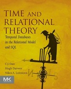
So, to continue with our example, let’s define a type MDATE that’s a proper subtype of type DDATE, where MDATE denotes dates that are accurate only to the month, not the day:
TYPE MDATE IS DDATE CONSTRAINT FIRST_OF_MONTH ( DDATE )
POSSREP MPRI { MI = THE_DI ( DDATE ) } POSSREP MPRC { MC = SUBSTR ( THE_DC ( DDATE ), 1, 7 ) } ;■ Type MDATE is defined to be a subtype of type DDATE, thanks to the specification IS DDATE.
■ In fact, a DDATE value is an MDATE value if and only if the DDATE value corresponds to the first of the month, thanks to the CONSTRAINT specification. (We’ve assumed the existence of an operator called FIRST_OF_MONTH that takes a value of type DDATE and returns TRUE if that value does indeed correspond to the first of the pertinent month, FALSE otherwise.)
■ Like type DDATE, type MDATE has two possreps, MPRI and MPRC, each of which is derived, in the manner specified, from the corresponding possrep for type DDATE. MPRC in particular allows us to think of MDATE values as if they were character strings of the form yyyy/mm. (In practice, we’d probably want to define yet another possrep for type MDATE, namely “month number,” again derived in some way from some possrep for type DDATE. We omit further consideration of this possibility for simplicity.)
Here now are the necessary selector and THE_ operators for type MDATE as just defined:
OPERATOR MPRI ( MI INTEGER ) RETURNS MDATE ;
/* code to return the MDATE value corresponding */
/* to the given integer MI (which must correspond */
/* in turn to the first of the month) */
END OPERATOR ;
OPERATOR THE_MI ( MD MDATE ) RETURNS INTEGER ;
/* code to return the integer corresponding */
/* to the given MDATE value MD */
END OPERATOR ;
OPERATOR MPRC ( MC CHAR ) RETURNS MDATE ;
/* code to return the MDATE value corresponding */
/* to the given yyyy/mm string MC */
END OPERATOR ;
OPERATOR THE_MC ( MD MDATE ) RETURNS CHAR ;
/* code to return the yyyy/mm string corresponding */
/* to the given MDATE value MD */
END OPERATOR ;
We’ve now defined type MDATE as a proper subtype of type DDATE (see the simple type hierarchy in Fig. 18.1). What are the implications of this fact? Probably the most important is the phenomenon known as value substitutability, which in the case at hand means that wherever the system expects a value of type DDATE, we can always substitute a value of type MDATE instead (because MDATE values are DDATE values). In particular, therefore, if Op is an operator that applies to DDATE values in general, we can always apply Op to an MDATE value specifically.4 For example, the operators “=”, THE_DI, and THE_DC defined above for values of type DDATE all apply to values of type MDATE as well (they’re inherited by type MDATE from type DDATE). Of course, the converse is false—operators specifically defined for values of type MDATE don’t apply to values of type DDATE (in general), because DDATE values aren’t MDATE values (again in general). We’ll see some examples in the next section.
It follows from the foregoing that, e.g., the following code fragment is valid:
VAR I INTEGER ;
VAR MDX MDATE ;
VAR DDX DDATE ;
I := THE_DI ( MDX ) ;
IF MDX = DDX THEN … END IF ;
/* etc., etc., etc. */
For simplicity, let’s assume for the remainder of this section that the type hierarchy contains just types DDATE and MDATE and no others. Given that assumption, let’s take a closer look at the fundamental operations of assignment (“:=”) and equality comparison (“=”). First, assignment. Consider the following example:
VAR DDX DDATE ;
DDX := MPRC ( '2013/09' ) ;
In the assignment here, the target variable on the left side is declared to be of type DDATE, but the source expression on the right side denotes a value of type MDATE. However, the assignment is valid, thanks to value substitutability. And after the assignment, of course, the variable contains a DDATE value that happens to satisfy the type constraint for type MDATE (to be specific, it contains the value DPRC (‘2013/09/01’), which is in fact an MDATE value). We can therefore say that, while the declared type of variable DDX is (as stated) DDATE, the current most specific type—i.e., the type of the current value of that variable—is MDATE. (That current value is of type DDATE as well, of course, because MDATE values are DDATE values. Thus, a given value has, in general, several types. As noted in Chapter 1, however, it always has exactly one most specific type.)
Now, it’s important to understand that the distinction we’re discussing here, between declared and current most specific types, applies not just to variable references but in fact to expressions in general. In other words, every expression has both a declared type and a current most specific type. To be specific, the declared type of an expression exp is, precisely, the declared type of the outermost operator involved in exp; likewise, the current most specific type of that same expression exp is, precisely, the current most specific type of the outermost operator invocation involved in the evaluation of exp.5 Note: The declared type of an operator is the type named in the RETURNS specification in the definition of the operator in question; the current most specific type of an invocation of that operator is the most specific type of the value returned by the invocation in question.
To continue with the code fragment shown above, suppose the following assignment is now executed:
DDX := DPRC ( '2012/10/17' ) ;
The current most specific type of variable DDX is now DDATE again, because the expression on the right side is of most specific type DDATE (i.e., it’s “only” of type DDATE, not type MDATE).
One more example:
DDX := DPRC ( '2000/11/01' ) ;
Here the DPRC invocation on the right side actually returns a value of type not just DDATE but MDATE, because the value in question satisfies the “first of month” constraint for type MDATE. We refer to this effect as specialization by constraint, on the grounds that the result of the DPRC invocation is “specialized” to type MDATE, precisely because it does satisfy the type constraint for type MDATE. And after the assignment, of course, the current most specific type of variable DDX is MDATE, too.
To generalize from the foregoing examples, let V be a variable of declared type T and let T' be a proper subtype of T. Then:
■ If the current most specific type of V is T and a value v of most specific type T' is assigned to V, the current most specific type of V becomes T' (as we’ve just seen). This effect is a logical consequence of the phenomenon we call specialization by constraint, as already explained.
■ Conversely, if the current most specific type of V is T' and a value v of most specific type T is assigned to V, the current most specific type of V becomes T. We refer to this effect as generalization by constraint, on the grounds that the current most specific type of V is “generalized” to type T—it’s established as T because the value v satisfies the type constraint for T and not for any proper subtype of T.
We note in passing that it’s precisely in this area (specialization by constraint and generalization by constraint) that the inheritance model we advocate [51-52] departs most obviously from other approaches described in the literature.
Be that as it may, you can see from the foregoing examples that it’s a rule regarding assignment that the most specific type of the source value can be any subtype (not necessarily a proper subtype, of course) of the declared type of the target variable. What about equality comparisons? In the absence of subtyping and inheritance, the comparison v1 = v2 would require the comparands v1 and v2 to be of the same type, T say. Thanks to value substitutability, however, we can substitute a value of any subtype of T for v1 and a value of any subtype of T for v2. It follows that for the comparison v1 = v2 to be legitimate, it’s necessary and sufficient that the most specific types of the comparands have a common supertype. Of course, the comparison will give true if and only if v1 and v2 are in fact the same value (implying in particular, therefore, that they’re of the same most specific type).
Point Types Revisited
Of course, there’s a lot more that could be said about type inheritance in general, but what we’ve said so far should suffice for the purposes of this chapter (for the time being, at any rate). Now let’s get back to point types as such. Now, it’s clear that type DDATE from the previous section can be made to meet all of the requirements for such a type if we want it to (and we do)—we can certainly define a total ordering based on a “>” operator for values of the type, and we can certainly define the necessary “first,” “last,” “next,” and “prior” operators as well. In fact, Tutorial D allows a type definition to state explicitly that the type in question is an ordinal type, as in this example (note the highlighted text):
TYPE DDATE ORDINAL
POSSREP DPRI { DI INTEGER CONSTRAINT DI ≥ 1 AND DI ≤ N } POSSREP DPRC { DC CHAR CONSTRAINT ………………… } ;The ORDINAL specification implies that “>”, “first,” “last,” “next,” and “prior” operators must all be explicitly defined for the type (a real language might require the names of those operators to be specified as part of the ORDINAL specification). Here are some possible definitions for those operators:
OPERATOR ">" ( DDI DDATE, DD2 DDATE ) RETURNS BOOLEAN ;
RETURN ( THE_DI ( DDI ) > THE_DI ( DD2 ) ) ;
END OPERATOR ;
OPERATOR FIRST_DDATE ( ) RETURNS DDATE ;
RETURN DPRI ( 1 ) ;
END OPERATOR ;
OPERATOR LAST_DDATE ( ) RETURNS DDATE ;
RETURN DPRI ( N ) ;
END OPERATOR ;
OPERATOR NEXT_DDATE ( DD DDATE ) RETURNS DDATE ;
RETURN DPRI ( THE_DI ( DD ) + 1 ) ;
END OPERATOR ;
OPERATOR PRIOR_DDATE ( DD DDATE ) RETURNS DDATE ;
RETURN DPRI ( THE_DI ( DD ) − 1 ) ;
END OPERATOR ;
Type DDATE now meets the sufficiency requirements for a point type. Note carefully, however, that the “first,” “last,” “next,” and “prior” operators are named FIRST_DDATE, LAST_DDATE, NEXT_DDATE, and PRIOR_DDATE, respectively.6 Although we did follow this style of naming in earlier chapters (“FIRST_T,” etc., where T is the name of the pertinent point type), we never really explained it properly, but now we need to, and we will.
Consider type MDATE. As we know, MDATE is a proper subtype of DDATE; thus, since DDATE is an ordinal type, we can regard MDATE as an ordinal type too, if we want to (and again we do want to, because we want to use type MDATE as a point type). So we need to define associated “>”, “first,” “last,” “next,” and “prior” operators for type MDATE. The “>” operator is inherited from type DDATE. So too are the operators NEXT_DDATE and so on; however, those operators are not the “next” (etc.) operators we need for type MDATE! For example, given the MDATE value August 1st, 2015, the operator NEXT_DDATE will return the date of the next day (August 2nd, 2015), not the date of the next month (September 1st, 2015). Thus, we need some new operators for type MDATE:
OPERATOR FIRST_MDATE ( ) RETURNS MDATE ;
RETURN MPRI ( op ( 1 ) ) ;
/* op ( 1 ) computes the integer possible representation */
/* —presumably 1—for the first day of the first month */
END OPERATOR ;
OPERATOR LAST_MDATE ( ) RETURNS MDATE ;
RETURN MPRI ( op ( N ) ) ;
/* op ( N ) computes the integer possible representation */
/* for the first day of the last month */
END OPERATOR ;
OPERATOR NEXT_MDATE ( MD MDATE ) RETURNS MDATE ;
RETURN MDATE ( THE_MI ( MD ) + incr ) ;
/* incr is 28, 29, 30, or 31, as applicable */
END OPERATOR ;
OPERATOR PRIOR_MDATE ( MD MDATE ) RETURNS MDATE ;
RETURN MDATE ( THE_MI ( MD ) - decr ) ;
/* decr is 28, 29, 30, or 31, as applicable */
END OPERATOR ;
And now we can see why the “first,” “last,” “next,” and “prior” operators for a given type T have to be named FIRST_T, LAST_T, NEXT_T, and PRIOR_T, respectively. For example, given the MDATE value August 1st, 2015, the operator NEXT_DDATE returns August 2nd, 2015 (as we already know); by contrast, the operator NEXT_MDATE returns September 1st, 2015. NEXT_DDATE and NEXT_MDATE are thus clearly different operators.
Aside: An alternative approach would be to call both NEXT_DDATE and NEXT_MDATE simply “NEXT” and provide two different implementation versions of that “NEXT” operator, using the mechanism—mentioned briefly in Chapters 7 and 8 and again in Chapter 17—called overloading. The expression NEXT (exp) would then cause the MDATE or DDATE implementation to be invoked according as to whether the type of exp was MDATE or just DDATE. (Note: The phrase “the type of exp” here could mean either the declared type or the most specific type, depending on factors beyond the scope of the present discussion.) However, such a scheme would do rather serious damage to an important prescription of our inheritance model—in terms of the DDATE and MDATE example, it could imply that there’d be no way to apply the DDATE version of NEXT to a value of type MDATE—and we therefore reject it. End of aside.
Numeric Point Types
Now we’d like to shift gears, as it were, and talk about the implications of the ideas discussed in this chapter so far for certain types that differ in kind, somewhat, from the calendar types DDATE and MDATE we’ve concentrated on prior to this point. To be specific, there are some languages—SQL is one—that support a variety of system defined NUMERIC types (where “numeric” really means fixed point decimal numbers, such 43.7 or −6.9). For example, the following is a legal SQL variable definition:
DECLARE V NUMERIC ( 5, 2 ) ;
Values of the specific numeric type illustrated here—i.e., NUMERIC(5,2)—are decimal numbers with precision five and scale factor two. In other words, those values are precisely the following:
-999.99, -999.98, …, -000.01, 000.00, 000.01, …, 999.99
In general, the precision for a given numeric type specifies the total number of decimal digits,7 and the scale factor specifies the position of the assumed decimal point, in the string of digits denoting any given value of the type in question, where:
■ A nonnegative scale factor q means the decimal point is assumed to be q decimal places to the left of the rightmost decimal digit of such a string of digits.
■ By contrast, a negative scale factor −q means the decimal point is assumed to be q decimal places to the right of the rightmost decimal digit of such a string of digits.
Note, therefore, that the precision and scale factor between them serve as an a priori constraint on values of the type; in effect, they constitute the applicable type constraint.
Aside: Observe that NUMERIC isn’t a type as such; instead, it’s a type generator. Specific numeric types such as NUMERIC(5,2) are obtained by invoking that type generator with arguments representing the desired precision and scale factor. End of aside.
We need to stress the fact that values of type NUMERIC(p,q) should be thought of as being denoted by strings of digits with an assumed decimal point. What this means is that if v is such a value, then v can be thought of in terms of a p-digit integer, n say; however, that p-digit integer n must be interpreted as denoting the value v = n * (10−q). The multiplier 10−q is the scale defined by the scale factor q (e.g., for NUMERIC(5,2), the scale is one hundredth).8 Observe that, by definition, every value of the type is evenly divisible by the scale (i.e., dividing the value in question by the scale always leaves a zero remainder). We note that the concept of scale can reasonably be applied to the examples of the previous section as well; for type DDATE it’s one day, for type MDATE it’s one month.
Note: From this point forward, we adopt the usual conventions regarding the omission of insignificant leading and trailing zeros in numeric literals. Thus, we might say more simply that the values of type NUMERIC(5,2) are:
−999.99, −999.98, …, −.01, 0, .01, …, 999.99
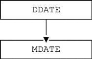
Fig. 18.2 gives several examples of NUMERIC types, with the corresponding scale and a symbolic picture of a typical value (ignoring the possible prefix minus sign) in each case.
■ Real languages usually provide a system defined type called INTEGER; indeed, we’ve been assuming the existence of just such a type throughout this book. However, we can now see that INTEGER is effectively just another spelling for NUMERIC(p,0) for some particular (system defined) precision p. Note: While every value of type INTEGER is certainly an integer, of course, it’s not the case that type INTEGER is the only type whose values are all integers. In fact, every type of the form NUMERIC(p,q) for which q is negative also has values that are all integers (see the next bullet item).
■ If the scale factor q is negative, least significant digits of the integer part of the number are missing. Those missing digits are assumed to be zeros. By way of example, values of type NUMERIC(3,−2) are:
−99900, −99800, …, −100, 0, 100, …, 99900
All of these values are numbers—in fact, integers—that are evenly divisible by one hundred, which is the scale.
Incidentally, we can use this example to highlight the important difference between a literal and a value (the concepts are indeed often confused—see, e.g., reference [11]). As explained in Chapter 1, a literal is not a value but is, rather, a symbol that denotes a value. Thus, e.g., the symbol 99900 is a literal that might on the face of it be thought of as denoting a value of type NUMERIC(5,0), not NUMERIC(3,−2). However, the value in question does happen to satisfy the type constraint for values of type NUMERIC(3,−2), which is, as we’ll see in a moment, actually a subtype of NUMERIC(5,0). Conceptually, therefore, specialization by constraint comes into play—at compile time, in fact—and the literal thus does indeed denote a value of type NUMERIC(3,−2). Similarly, the literal 5.00 actually denotes a value of type INTEGER. See the discussion of multiple inheritance later in this section for further discussion.
■ If the scale factor q is greater than the precision p, most significant digits of the fractional part of the number are missing. Again, those missing digits are assumed to be zeros. By way of example, values of type NUMERIC(3,5) are:
−0.00999, −0.00998, …, −0.00001, 0.0, 0.00001, …, 0.00999
(Here we do show the zero integer part preceding the decimal point, just for explicitness.) All of these values are numbers that are evenly divisible by one hundred thousandth, which is the scale.
Now, it’s surely obvious that any of these NUMERIC types can be used as a point type, and we’ll examine that possibility in a few moments. However, there’s an important issue that needs to be addressed first, as follows:
■ Consider the types NUMERIC(3,1) and NUMERIC(4,1). It should be clear that every value of type NUMERIC(3,1) is a value of type NUMERIC(4,1) as well9—to be specific, a value of type NUMERIC(4,1) for which the leading digit in the integer part happens to be zero. It follows that NUMERIC(3,1) is a proper subtype of NUMERIC(4,1), and so we can (for example) assign a value of the former type to a variable that’s declared to be of the latter type.
■ Now consider the types NUMERIC(3,1) and NUMERIC(4,2). It should also be clear that every value of type NUMERIC(3,1) is a value of type NUMERIC(4,2) as well10—to be specific, a value of type NUMERIC(4,2) for which the trailing digit in the fractional part happens to be zero. It follows that NUMERIC(3,1) is a proper subtype of NUMERIC(4,2) as well.
■ Observe now that neither of NUMERIC(4,1) and NUMERIC(4,2) is a subtype of the other; for example, 999.9 is a value of the first type that’s not a value of the second, while 99.99 is a value of the second type that’s not a value of the first. And so we see that type NUMERIC(3,1) has two distinct proper supertypes, neither of which is a subtype of the other. It follows that here we’re dealing with multiple inheritance—i.e., a form of inheritance in which a given type can have n proper supertypes, none of which is a subtype of any other, for some n > 1. (By contrast, the form of inheritance discussed earlier in this chapter was, tacitly, what’s called single inheritance only. Of course, single inheritance is just a degenerate special case of multiple inheritance.)
Thus, we need to digress again for a moment in order to extend the ideas presented earlier for single inheritance to deal with the possibility of multiple inheritance.
Multiple Inheritance
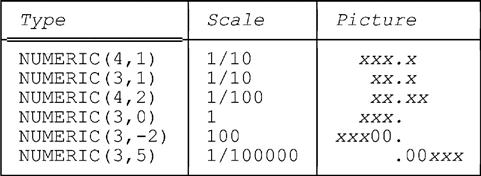
Consider the case of numeric types once again. Assume for definiteness and simplicity that the maximum precision the system supports is 3 (the minimum, of course, is 1) and the maximum and minimum scale factors are 4 and −4, respectively. Then Fig. 18.3 shows the corresponding type lattice—a simple type hierarchy will obviously no longer suffice—for the entire range of valid numeric types. (For space reasons, we abbreviate the type name “NUMERIC(p,q)” throughout that figure to just “p,q”.) The figure should be more or less self-explanatory, except for the two types LUB and GLB shown at the top and bottom of the lattice, respectively, which we now explain:
■ Type LUB (“least upper bound”) contains all possible NUMERIC values and is a proper supertype of every other type in the figure.11
■ Type GLB (“greatest lower bound”), by contrast, is a type that contains just the single value zero; it’s a proper subtype of every other type in the figure.
What extensions are needed to our model of inheritance as sketched earlier in order to deal with situations like the one illustrated in Fig. 18.3? It turns out that—at least so far as we’re concerned in the present book—not many extensions are needed at all. In fact, the only one we need consider here is this:
■ If types T1 and T2 overlap (i.e., have at least one value in common), then they must have both:
b. A common subtype T' (the intersection type for T1 and T2) such that every value that’s of both type T1 and type T2 is in fact a value of type T'.
(Actually the foregoing statement is both simpler and more complicated than it really needs to be—simpler, because among other things it needs to be generalized to deal with three or more overlapping types; more complicated, because if the proper groundwork is laid first, it can be stated much more elegantly and precisely. See reference [51] for further discussion.)
Observe now that the foregoing rule is certainly satisfied in Fig. 18.3. For example, consider the types NUMERIC(2,1) and NUMERIC(2,0). These two types do overlap—for example, they have the value 9 in common. And:
a. They do have a common supertype, NUMERIC(3,1).
b. They also have a common subtype, NUMERIC(1,0), such that a value is of both the specified types if and only if it’s a value of that common subtype.12
The foregoing rule regarding overlapping types can be regarded as a rule that type lattices like that in Fig. 18.3 are required to obey in order to be well formed. And, assuming the type lattice we have to deal with is indeed well formed in this sense, we can now say that:
■ Our previous rule regarding assignment remains unchanged: namely, the most specific type of the source must be some subtype of the declared type of the target.
■ What’s more, our previous rule for equality comparison remains unchanged, too: The most specific types of the comparands must have a common supertype. However, this latter rule now has an extended interpretation. For example, it’s possible that a comparison between a NUMERIC(2,1) value and a NUMERIC(2,0) value might give true—but only if the values in question are in fact both of the corresponding intersection type NUMERIC(1,0) (and are both the same value, of course).
Point Types Continued
Now let’s get back to the main topic of this chapter. Clearly, all of the various numeric types we’ve been discussing can be used as point types—they all have a total ordering, and “first,” “last,” “next,” and “prior” operators can obviously be defined for all of them. However, they differ in one significant respect from types DDATE and MDATE as discussed earlier, inasmuch as the definitions of the “first” (etc.) operators are all effectively implied by the applicable precision and scale—the precision implies the definitions of the “first” and “last” operators, and the scale implies the definitions of the “next” and “prior” operators. For example, consider the type NUMERIC(3,1), which consists of the following values (in order):
−99.9, −99.8, …, −0.1, 0, 0.1, …, 99.9
Clearly, the “first” operator here returns −99.9, the “last” operator returns 99.9, the “next” operator is “add one tenth,” and the “prior” operator is “subtract one tenth.”
Aside: To be consistent with our earlier remarks regarding operator naming, the foregoing operators ought by rights to be named FIRST_NUMERIC(3,1), LAST_NUMERIC(3,1), NEXT_NUMERIC(3,1), and PRIOR_NUMERIC(3,1), respectively! Quite apart from the question as to whether such names are even syntactically legal, we’d be the first to admit that they’re clumsy and ugly. However, as we’ve said elsewhere in this book, we’re concerned here not so much with matters of concrete syntax, but rather with the question of getting the conceptual foundations right. And conceptually, yes, the “first,” “last,” “next,” and “prior” operators for type NUMERIC(3,1) really are different from the corresponding operators for (e.g.) type NUMERIC(4,2), and they do need different names. (If they need names at all, that is—but they might not. For example, the expression NEXT_NUMERIC(3,1) (exp), where exp is of declared type NUMERIC(3,1), will clearly return the same result as the expression exp + 0.1. Thus, the conventional “+” operator might be all we need here.13 Note too that even though the declared type of the expression exp + 0.1 will probably be just LUB, the result it returns at run time will certainly be of type NUMERIC(3,1)—and possibly some proper subtype thereof—thanks to specialization by constraint.) End of aside.
Other Scales
In effect, what we’ve been claiming in our discussion so far is this: To say a certain NUMERIC type has a certain precision and scale is really just a shorthand way of saying we have a type that (a) is usable as a point type, (b) has values that are numbers, and (c) has certain specific “first,” “next,” etc., operators. We now observe, however, that this shorthand—what we might call “the NUMERIC(p,q) shorthand”—works only if the desired scale is a power of ten. But other scales are certainly possible, and perhaps desirable, even with types that are essentially numeric in nature. We now briefly consider this possibility.
By way of a simple example, suppose we want a point type consisting of even integers—which is to say, an ordinal type for which (a) the values are (let’s agree) the integers −99998, −99996, …, −2, 0, 2, …, 99998, and (b) the “first,” “next,” etc., operators are as suggested by this sequence (i.e., the “first” operator returns −99998, the “next” operator is “add two,” and so on). No NUMERIC(p,q) shorthand is capable of expressing these requirements. Instead, therefore, we need to define an explicit subtype, perhaps as follows:
TYPE EVEN_INTEGER ORDINAL
IS INTEGER CONSTRAINT MOD ( INTEGER, 2 ) = 0 … ;
MOD here (“modulo”) is, let’s assume, an operator that takes two integer operands and returns the remainder that results after dividing the first by the second. (The reference to the type name “INTEGER” in the CONSTRAINT specification is meant to stand for an arbitrary value of type INTEGER.)
The “=” and “>” operators for EVEN_INTEGER are inherited from type INTEGER. As for the “first” (etc.) operators, they might be defined as follows:
OPERATOR FIRST_EVEN_INTEGER ( ) RETURNS EVEN_INTEGER ;
RETURN −99998 ;
END OPERATOR ;
OPERATOR LAST_EVEN_INTEGER ( ) RETURNS EVEN_INTEGER ;
RETURN 99998 ;
END OPERATOR ;
OPERATOR NEXT_EVEN_INTEGER ( I EVEN_INTEGER ) RETURNS EVEN_INTEGER ;
RETURN I + 2 ;
END OPERATOR ;
OPERATOR PRIOR_EVEN_INTEGER ( I EVEN_INTEGER ) RETURNS EVEN_INTEGER ;
RETURN I − 2 ;
END OPERATOR ;
Aside: Actually we’ve taken some rather considerable liberties in these operator definitions. The fact is that, e.g., the expression in the RETURN statement in the definition of FIRST_EVEN_INTEGER ought really to be, not just the literal −99998 as shown, but rather an expression of the form TREAT_AS_EVEN_INTEGER (−99998). However, detailed discussion of this point would take us much further away from our main topic than we care to go here; thus, we’ve adopted certain simplifications in order to avoid a detailed discussion of a subject that’s not very relevant to our main purpose.14 For further discussion and explanation, see reference [51]. End of aside.
In the same kind of way, we might define, e.g., a point type where the scale is calendar quarters and the “next” operator is “add three months,” or a point type where the scale is decades and the “next” operator is “add ten years” (and so on).
Granularity Revisited
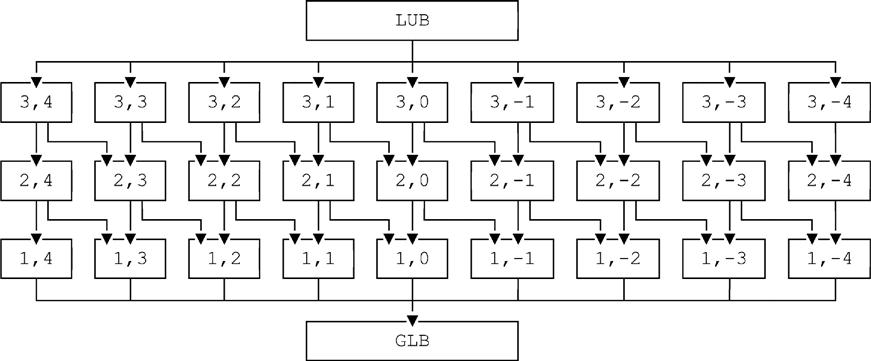
We now turn our attention to the concept of granularity. Recall from Chapter 4 that this term refers, informally, to the “size” of the individual points, or equivalently the size of the gap between adjacent points, for the point type in question. Fig. 18.4 lists the various point types we’ve been considering in this chapter so far, with (a) their scales as previously discussed and also with (b) their corresponding granularities.
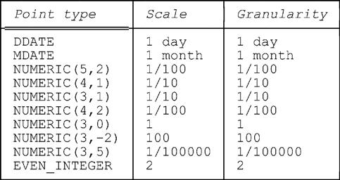
Now, you might have noticed that we didn’t mention the term granularity in previous sections of this chapter at all. One major reason for that omission is that, in all of the examples discussed in this chapter so far, the granularity is identical to the corresponding scale, as Fig. 18.4 clearly shows. For those types, therefore, the term is simply redundant; it’s just another term for a concept for which a better term already exists (not to mention the fact that scale is formally defined, while—pace references [6] and [62]—granularity seems not to be). However, a more important reason for the omission is that there are some point types for which the concept of granularity doesn’t apply. We’ll give an example in a few moments. First, however, we want to consider a different example, involving a user defined type called HEIGHT. Here’s the definition:
TYPE HEIGHT POSSREP HIPR { HI INTEGER CONSTRAINT HI > 0 AND HI ≤ 120 } ;Type HEIGHT is meant to represent person heights. Legal values are as follows:
HIPR ( 1 ), HIPR ( 2 ), …, HIPR ( 120 )
These values are meant to denote heights in inches (we’re assuming nobody is under one inch or over ten feet tall). Clearly, the granularity is one inch. Or is it? Surely we might equally well say it’s two half-inches, or one twelfth of a foot—or even 2.54 centimeters, or 25.4 millimeters, or any of many, many other possibilities. Thus, we see that, in general, granularity requires some associated unit of measure (not necessarily unique) in order for it to make sense.
Of course, while there might be many different ways, some of which might be more user friendly than others, of stating what the granularity actually is in any given situation, those different ways must all be logically equivalent to one another—which is just as well, in fact, since the concept of units of measure has no formal part to play in a type definition. Indeed, reference [52] argues that, as a general rule, types and units should generally not be in any kind of one to one correspondence. That is, instead of having (e.g.) one type representing heights in inches and another representing heights in centimeters, it would be better to have just one HEIGHT type with two distinct possreps, one for inches and one for centimeters. But now we’re beginning to stray too far from our main topic once again. To return to that topic, we now show (as promised) an example of a point type for which the granularity concept doesn’t seem to apply at all:
TYPE RICHTER ORDINAL
POSSREP RPR { R NUMERIC ( 3, 1 ) CONSTRAINT R > 0.0 } ;Type RICHTER is meant to represent points on the Richter scale. Legal values are as follows:
RPR ( 0.1 ), RPR ( 0.2 ), … , RPR ( 1.0 ),
RPR ( 1.1 ), RPR ( 1.2 ), … ,
………………………… , RPR ( 99.9 ) /* help! */
As is well known, however, the Richter scale is not linear but logarithmic to base 10.15 As a consequence, it makes little sense to talk about the concept of “granularity” in this context at all—the gaps between one RICHTER value and the next aren’t of constant size.16 So what this example demonstrates is that there’s a logical difference between scale and granularity:
■ Scale is, as already stated, a formal concept; essentially, it’s the basis of the definition of the successor function (“next”).
■ Granularity, by contrast, is an informal concept only; it helps to explain at an intuitive level what a certain point type is supposed to represent. However, it does tacitly assume that the point type in question involves evenly spaced values.
In other words, the tacit model underlying the concept of granularity seems to be something like the following:
■ We’re given a linear axis (e.g., “the timeline”) with certain points marked on it.
■ Those marked points are the only ones of interest—there are no accessible points “between” adjacent points on the axis. To put it another way, measurements along the axis are discrete, not continuous (they always correspond to one of the marked points, there are no “half measures”).
■ Those points of interest are assumed to be evenly spaced along the axis. That is, if p1 and p2 are any two adjacent points, then the size g of the gap between p1 and p2—which must be measured, be it noted, by going outside the model—is always the same.
■ That constant value g is the granularity. Furthermore, it corresponds to the scale, in the sense that g is what must be “added” to any given point to get to the next.
But the RICHTER example shows that the even spacing assumption isn’t always valid. For type RICHTER, scale makes sense, but granularity does not. More generally, whenever granularity makes sense, then scale does too, but the converse is false.
We now consider one last example of a point type in order to show that, not only does granularity not always apply, but scale doesn’t always apply either:
TYPE PRIME ORDINAL IS INTEGER CONSTRAINT … ;
Values of type PRIME are (let’s agree) prime numbers, starting with two; the CONSTRAINT specification, details of which are omitted for simplicity, presumably consists of a reference to some operator that determines, for any given positive integer p, whether p is in fact prime.
Now, prime numbers are certainly not regularly spaced, so the concept of granularity doesn’t apply. What’s more, there’s no obvious scale, either! And yet PRIME is clearly usable as a point type—”>“ is obviously applicable, and we can define suitable “first” (etc.) operators, thus:
OPERATOR FIRST_PRIME ( ) RETURNS PRIME ;
RETURN 2 ;
END OPERATOR ;
OPERATOR LAST_PRIME ( ) RETURNS PRIME ;
RETURN N ; /* N = the largest representable prime */
END OPERATOR ;
OPERATOR NEXT_PRIME ( P PRIME ) RETURNS PRIME ;
/* code to compute the prime immediately following P */
END OPERATOR ;
OPERATOR PRIOR_PRIME ( P PRIME ) RETURNS PRIME ;
/* code to compute the prime immediately preceding P */
END OPERATOR ;
So PRIME is an example of a type that’s certainly usable as a point type and yet has no scale (and a fortiori no granularity).17
To summarize: The concept of granularity (a) isn’t formally defined, (b) doesn’t always apply, and (c) seems to be identical to the concept of scale when it does apply. Given this state of affairs, it seems a little strange that the concept has received so much attention in the literature—especially since, as noted in Chapter 4, there seems to be a certain amount of confusion surrounding the concept anyway; for example, it’s sometimes taken to be the same as precision (!). By way of a second example (i.e., of apparent confusion), you might like to meditate on the following definition from reference [62]. Italics are as in the original.
[The] timestamp granularity is the size of each chronon in a timestamp interpretation. For example, if the timestamp granularity is one second, then the duration of each chronon in the timestamp interpretation is one second (and vice versa) … If the context is clear, the modifier “timestamp” may be omitted.
Note: The concept of “timestamp interpretation” is defined elsewhere in the same document thus:
[The] timestamp interpretation gives the meaning of each timestamp bit pattern in terms of some time-line clock chronon (or group of chronons).
(The term chronon was discussed briefly in Chapter 4.)
Interval Types Revisited
In Chapter 6, we defined an interval type to be, specifically, a generated type of the form INTERVAL_T, where T is a point type. Like all generated types, therefore, interval types have certain generic operators associated with them: specifically, interval selectors, BEGIN and END, PRE and POST, POINT FROM, “∈” and “∋”, COUNT, Allen’s operators, and interval UNION, INTERSECT, and MINUS. In this section, we consider some of the implications of the ideas discussed so far in this chapter on these operators.
We begin our investigation by noting that if T is a point type and T is a proper subtype of T, then INTERVAL_T' is not a subtype of INTERVAL_T. Why not? Because intervals of type INTERVAL_T' aren’t intervals of type INTERVAL_T. Indeed, even if intervals i and i', of types INTERVAL_T and INTERVAL_T' respectively, have the same begin and end points b and e, they’re not the same interval, because they have different sets of contained points (except in the special case where b = e, meaning the interval in question is a unit interval). For example, take T and T' as INTEGER and EVEN_INTEGER, respectively, and consider i = [2:6] and i' = [2:6]; then i contains the integers 2, 3, 4, 5, and 6, while i' contains just the even integers 2, 4, and 6.
Note: Even in that special case where b = e, intervals i and i' are still not the same interval, precisely because they’re of different types. For example, the operator invocations POST(i) and POST(i') will give different results, even in this special case (unless e happens to be the last value of both types T and T', of course, in which case the POST invocations are both undefined).
One important consequence of the foregoing is that the type of a given interval can’t be inferred from the type of its begin and end points. It follows that—as indeed we already know from earlier chapters—interval selectors do need that “_T" qualifier, just as the “first” and “next” (etc.) operators do. Here are a couple of examples:
INTERVAL_INTEGER ( [2:6] )
INTERVAL_EVEN_INTEGER ( [2:6] )
The general format—assuming, as usual, closed:closed notation just for definiteness—is INTERVAL_T ([b:e]), where b and e are values of type T and b ≤ e.
A more general consequence is as follows. We’ve seen in particular that if T' is a proper subtype of T, then INTERVAL_T' isn’t a subtype of INTERVAL_T. In fact, if IT is the interval type INTERVAL_T, then in general there’s no interval type of the form INTERVAL_T'—let’s call it IT'—that’s a proper subtype of IT. For suppose, conversely, that such a type IT' does in fact exist. Let i' = [b’:e] be an interval of type IT' such that b' ≠ e'. Since IT' is a subtype of IT, i' must be an interval of type IT as well. But even if b' and e'’happen to be values of type T, i' can’t possibly be an interval of type IT, because its contained points are determined by the successor function for T', which by definition is distinct from the successor function for T. Contradiction!
Note: The remarks in the foregoing paragraph are broadly true, but there are some minor exceptions that we should at least mention in passing:
■ First, if T' is empty—see the answer to Exercise 6.5 in Chapter 6—then IT' is a subtype of all possible interval types; in fact, it’s a proper subtype of all of them except for IT' itself. However, IT', like T', is empty in this case (it contains no intervals).
■ Second, if T' is a singleton type whose sole value is a value of type T—again see the answer to Exercise 6.5 in Chapter 6—then IT' is a subtype of IT after all, but it contains just one interval (necessarily a unit interval, of course).
■ Third (and perhaps more important than the previous two possibilities), it might be possible to define a type IT' that is a proper subtype of IT—for example, IT' might be defined to consist of just those intervals of type IT that happen to be unit intervals—but if T contains at least two points, then such a type IT' can’t be defined by means of the interval type generator. Thus, it wouldn’t be a type (a generated type, that is) of the form INTERVAL_T' as such. Please note, therefore, that (as we’ve more or less said already) when we use the term interval type in this book, we always mean, specifically, a type that’s produced by some invocation of the INTERVAL type generator.
Next, we observe that intervals are of course values; like all values, therefore, they carry their type around with them, so to speak. Thus, if i is an interval, it can be thought of as carrying around with it a kind of flag that announces “I’m an interval of type INTERVAL_INTEGER” or “I’m an interval of type INTERVAL_EVEN_INTEGER” or “I’m an interval of type INTERVAL_DDATE” (etc., etc.). In fact, if we ignore the minor exceptions identified above, we can reasonably say that every interval carries exactly one type with it, and so we can speak unambiguously of the type of any given interval. (That type is of course the most specific type of the interval in question, but in effect it’s the least specific type too, and indeed the declared type of any expression denoting it as well.)
Now consider the operator POST, which, given the interval i = [b:e], returns the immediate successor e+1 of the end point e of i. Now, the type of the argument i here is known and well defined; hence the applicable successor function is known as well, and so there’s no need for POST to involve any kind of _T qualifier. Thus, the following is a valid POST invocation:
POST ( INTERVAL_INTEGER ( [2:6] ) )
The result, of course, is 7. By contrast, the POST invocation
POST ( INTERVAL_EVEN_INTEGER ( [2:6] ) )
returns 8, not 7.
It should be clear that remarks analogous to the foregoing apply equally to PRE, BEGIN, END, and indeed to all of the other generic interval operators, because the applicable successor function, when needed, is always known. In other words, the only interval operators that require that _T qualifier are interval selectors. (In fact, of course, interval selectors differ in kind from the other operators mentioned, inasmuch as their operands are points, not intervals. In this respect, they resemble the operators “first,” “last,” “next,” and “prior,” all of which take operands that are points, and all of which do need that _T qualifier.)
Allen’s Operators Revisited
Suppose we’re given three point types T, T1, and T2, such that T1 and T2 are distinct proper subtypes of T. To make the example a little more concrete, take T to be INTEGER, and take T1 and T2 to be “integers that are multiples of two” and “integers that are multiples of three,” respectively.18 Now let p1 be a value (point) of type T1 and let p2 be a value of type T2. As we already know, then, the comparison
p1 = p2
is certainly legal, and might even give TRUE (e.g., suppose p1 and p2 are both 18). Moreover, the comparison
p1 > p2
is also legal—at least, it would be unreasonable to define “>“ in such a way as to make it not so—and of course it might give TRUE as well (e.g., suppose p1 is 14 and p2 is 9).
Given the foregoing state of affairs, let’s see whether it makes any sense to generalize Allen’s operators accordingly. For brevity, let’s agree to use the shorthand names IT, IT1, and IT2 to denote the interval types INTERVAL_T, INTERVAL_T1, and INTERVAL_T2, respectively. Then:
■ Let i1 = [b1:e1] be an interval of type IT1. Define j1 = [b1:e1] to be the unique interval of type IT with the same begin and end points as i1. For example, if b1 and e1 are 2 and 6, respectively, then i1 contains just the points 2, 4, and 6, while j1 contains the points 2, 3, 4, 5, and 6.
■ Similarly, let i2 = [b2:e2] be an interval of type IT2, and define j2 = [b2:e2] to be the unique interval of type IT with the same begin and end points as i2.
Now let Op denote any of Allen’s operators apart from “=”; then we can define i1 Op i2 to be logically equivalent to j1 Op j2—though whether we’d really want to do so is another matter! Anyway, let’s see how this proposed definition works out for each of the operators in turn:
■ Inclusion: Let i1 and i2 be [4:8] and [3:12], respectively. Then i1 ⊂ i2 is true, and so of course are i1 ⊆ i2, i2 ⊃ i2, and i2 ⊇ i2. Note, however, that (e.g.) i1 ⊂ i2 does not mean in this context that every point in i1 is also a point in i2, a state of affairs that might immediately give us pause … Do we really want to go down this path? Well, let’s overlook such reservations and continue, at least for now.
■ BEFORE and AFTER: Let i1 and i2 be [4:6] and [9:18], respectively. Then i1 BEFORE i2 is true, and so of course is i2 AFTER i1.
■ OVERLAPS: Let i1 and i2 be [4:10] and [9:18], respectively. Then i1 OVERLAPS i2 and i2 OVERLAPS i1 are both true—despite the fact that i1 and i2 have no points in common!
■ MEETS: Let i1 and i2 be [4:8] and [9:18], respectively. Then i1 MEETS i2 and i2 MEETS i1 are both true.
■ MERGES: As usual, i1 MERGES i2 is true if and only if i1 OVERLAPS i2 is true or i1 MEETS i2 is true (but OVERLAPS and MEETS now have extended definitions).
■ BEGINS and ENDS: Let i1 and i2 be [6:10] and [6:18], respectively. Then i1 BEGINS i2 is true. Similarly, let i1 and i2 be [14:18] and [6:18], respectively. Then i2 ENDS i1 is true.
It follows from all of the above that we can generalize the interval union, intersection, and difference operators as well (again, if we want to):
■ UNION: The definition remains unchanged—i1 UNION i2 is defined if and only if i1 MERGES i2 is true, in which case it returns [MIN{b1,b2}:MAX{e1,e2}]. Note, however, that the result is of type IT, not IT1 or IT2. For example, let i1 and i2 be [4:10] and [9:18], respectively; then i1 UNION i2 is [4:18], containing the following points:
4, 5, 6, 7, 8, 9, 10, 11, 12, 13, 14, 15, 16, 17, 18
■ INTERSECT: Again the definition remains unchanged—i1 INTERSECT i2 is defined if and only if i1 OVERLAPS i2 is true, in which case it returns [MAX{b1,b2}:MIN{e1,e2}]. Again, however, that the result is of type IT, not IT1 or IT2. For example, let i1 and i2 be [4:10] and [9:18], respectively; then i1 INTERSECT i2 is [9:10], containing just the following points:
9, 10
■ MINUS: Yet again the definition remains effectively unchanged—i1 MINUS i2 is defined if and only if (a) i1 OVERLAPS i2 is false (in which case i1 MINUS i2 reduces to simply i1), or (b) j1 (not i1) contains either b2 or e2 but not both, or (c) exactly one of i2 BEGINS i1 and i2 ENDS i1 is true. Once again, however, the result is of type IT, not IT1 or IT2. For example, let i1 and i2 be [4:10] and [9:18], respectively; then i1 MINUS i2 is [4:8], containing just the following points:
4, 5, 6, 7, 8
Finally, recall that the all important PACK operator is defined in terms of interval union and intersection, and so it follows that PACK too can be generalized along the foregoing lines. (So of course can UNPACK.) We leave the specifics as something for you to think about, if you’re interested. Our own feeling, though, for what it’s worth, is that these various generalized definitions—starting with interval inclusion and continuing with OVERLAPS, MEETS, and so on—display so much in the way of anomalous behavior that it would be better not to support them after all.
Concluding Remarks
In this chapter, we’ve examined, among many other things, type inheritance, both single and multiple—at least insofar as that concept applies to point and interval types—and the associated notions of ordering, precision, scale, successor function, and granularity. These various concepts, though distinct, are very much interwoven; in fact, they’re interwoven in rather complicated ways, and it can sometimes be quite difficult to say just where the demarcations lie. What we’ve tried to do is pin down the distinctions among them (the concepts, that is) as precisely as possible, and thereby shed some light on a subject on which much of the existing literature seems to be very confusing—not to say confused.
Exercises
18.1 Define in your own terms:
b. Specialization by constraint
c. Generalization by constraint
18.2 What do you understand by the term multiple inheritance?
18.3 Let CHAR(n) denote a type whose values are character strings of at most n characters. Does CHAR(n) make sense as a point type?
18.4 Define a point type called MONEY, with the obvious semantics. Give definitions for all associated selectors and THE_ operators, also for the successor function and related operators (FIRST_MONEY, NEXT_MONEY, etc.).
18.5 Extend your answer to Exercise 18.4 to incorporate the necessary support for two distinct monetary scales, one expressed in terms of (say) dollars and the other in terms of cents.
Answers
a. Substitutability is a term used in connection with operator invocations. It refers to the substitution of arguments, in the invocation in question, for the parameters of the operator in question. Let Op be an operator, let P be a parameter to Op, and let P be of declared type T. Further, let P not be subject to update. Then The Principle of Value Substitutability allows the argument (a value) substituted for P in any given invocation of Op to be of any subtype of T.
Suppose now that P is subject to update (so the corresponding argument expression is required to be a variable reference specifically). A Principle of Variable Substitutability, analogous to The Principle of Value Substitutability, would say that wherever an argument variable of type T is expected, a variable of any proper subtype of T is also permitted. In that case, it would be permitted, for example, to assign a value of type RECTANGLE to a variable of declared type SQUARE. Since rectangles generally aren’t squares, such an assignment should clearly fail at run time, if not at compile time. For such reasons, a Principle of Variable Substitutability isn’t normally adopted. Note: Object oriented languages typically do, however, allow such “variable substitutability” for certain special kinds of variables known as objects. They do so, somewhat suspectly, by not allowing invocations of update operators on such variables to give rise to a change of most specific type. One consequence of this approach is that if you define an “object class” called SQUARE, you must be prepared to deal with the fact that objects of that class might not correspond to squares in the real world but only to rectangles (because adjacent sides are of different lengths).
b. Specialization by constraint is the phenomenon whereby the result x of evaluating an expression of declared type T might have types T1, T2, …, Tn in addition to type T, by virtue of the fact that each of T1, T2, …, Tn is a proper subtype of T such that x satisfies the constraint that defines the values constituting that subtype.
c. Generalization by constraint is the phenomenon whereby the result x of evaluating an expression to be assigned to variable V of declared type T might cause the most specific type of V—necessarily a subtype of T—to be some proper supertype of the most specific type of the value being replaced by x.
18.2 Multiple inheritance is a term denoting the possibility that a type might have two or more distinct immediate supertypes—where type T is an immediate supertype of type T' if and only if it’s a proper supertype of T' and there’s no type T”, distinct from both T and T', such that T is a proper supertype of T”and T” is a proper supertype of T'. Note: If and only if T is an immediate supertype of T', then T' is an immediate subtype of T.
18.3 Let the characters in the character set from which strings of type CHAR(n) are drawn be totally ordered, with Ic as the least character in that ordering and ɡc as the greatest, and let string comparisons be done in the usual way, character by character from left to right. Then FIRST_CHAR(n) is the empty string and LAST_CHAR(n) is the string consisting of n occurrences of the character ɡc. For a given string s ≠ LAST_CHAR(n), of length Is, NEXT_CHAR(s) could be defined as follows:
Case 1: When Is < n, then s concatenated with Ic.
Case 2: When Is = n and the rightmost character of s isn’t ɡc, then the string formed by replacing that rightmost character by its immediate successor.
Case 3: When Is = n and the rightmost k characters of s are all ɡc, then the string consisting of the leftmost Is − (k + 1) characters of s followed by the character that’s the immediate successor of the (Is − k)th character of s.
Therefore CHAR(n) is usable as a point type.19 But does it make any sense as a point type? Possibly, and intervals such as INTERVAL_CHAR(30) ([‘Darwen’:‘Date’]) might have some useful application. However, counterintuitive results might arise from the fact that, for example, ‘Daszzzzzzzzzzzzzzzzzzzzzzzzzzz’ is a string in that interval.
Have you heard the one about the person who, looking in the bookstore for a book on hypnotism, discovered and bought the one titled Guide to Hypnotism? Disappointment ensued when she discovered she had purchased Volume 6 of a certain encyclopedia.
18.4 TYPE MONEY ORDINAL POSSREP DOLLARS_AND_CENTS { D_AND_C NUMERIC(9,2) } ;
OPERATOR DOLLAR_AND_CENTS ( D_AND_C NUMERIC(9,2) ) RETURNS MONEY ;
/* code to return the MONEY value corresponding */
/* to the given NUMERIC(9,2) value D_AND_C */
END_OPERATOR ;
OPERATOR THE_D_AND_C ( AMOUNT MONEY ) RETURNS NUMERIC(9,2) ;
/* code to return the NUMERIC(9,2) value corresponding */
/* to the given MONEY value AMOUNT */
END OPERATOR ;
OPERATOR "=" ( A1 MONEY, A2 MONEY ) RETURNS BOOLEAN ;
RETURN ( THE_D_AND_C ( A1 ) = THE_D_AND_C ( A2 ) ) ;
END OPERATOR ;
OPERATOR ">" ( A1 MONEY, A2 MONEY ) RETURNS BOOLEAN ;
RETURN ( THE_D_AND_C ( A1 ) > THE_D_AND_C ( A2 ) ) ;
END OPERATOR ;
OPERATOR FIRST_MONEY ( ) RETURNS MONEY ;
RETURN DOLLARS_AND_CENTS ( −9999999.99 ) ;
END OPERATOR ;
OPERATOR LAST_MONEY ( ) RETURNS MONEY ;
RETURN DOLLARS_AND_CENTS ( 9999999.99 ) ;
END OPERATOR ;
OPERATOR NEXT_MONEY ( AMOUNT MONEY ) RETURNS MONEY ;
RETURN DOLLARS_AND_CENTS ( THE_D_AND_C ( AMOUNT ) + 0.01 )
END OPERATOR ;
OPERATOR PRIOR_MONEY ( AMOUNT MONEY ) RETURNS MONEY ;
RETURN DOLLARS_AND_CENTS ( THE_D_AND_C ( AMOUNT ) − 0.01 )
END OPERATOR ;
18.5 TYPE CMONEY ORDINAL POSSREP DOLLARS_AND_CENTS { D_AND_C NUMERIC(9,2) } ;
OPERATOR DOLLARS_AND_CENTS ( D_AND_C NUMERIC(9,2) ) RETURNS CMONEY ;
/* code to return the CMONEY value corresponding */
/* to the given NUMERIC(9,2) value D_AND_C */
END_OPERATOR ;
OPERATOR THE_D_AND_C ( AMOUNT CMONEY ) RETURNS NUMERIC(9,2) ;
/* code to return the NUMERIC(9,2) value corresponding */
/* to the given CMONEY value AMOUNT */
END_OPERATOR ;
OPERATOR "=" ( A1 CMONEY, A2 CMONEY ) RETURNS BOOLEAN ;
RETURN ( THE_D_AND_C ( A1 ) = THE_D_AND_C ( A2 ) ) ;
END_OPERATOR ;
OPERATOR ">" ( A1 CMONEY, A2 CMONEY ) RETURNS BOOLEAN ;
RETURN ( THE_D_AND_C ( A1 ) > THE_D_AND_C ( A2 ) ) ;
END_OPERATOR ;
OPERATOR FIRST_CMONEY ( ) RETURNS CMONEY ;
RETURN DOLLARS_AND_CENTS ( −9999999.99 ) ;
END_OPERATOR ;
OPERATOR LAST_CMONEY ( ) RETURNS CMONEY ;
RETURN DOLLARS_AND_CENTS ( 9999999.99 ) ;
END_OPERATOR ;
OPERATOR NEXT_CMONEY ( AMOUNT CMONEY ) RETURNS CMONEY ;
RETURN DOLLARS_AND_CENTS ( THE_D_AND_C ( AMOUNT ) + 0.01 ) ;
END_OPERATOR ;
OPERATOR PRIOR_CMONEY ( AMOUNT CMONEY ) RETURNS CMONEY ;
RETURN DOLLARS_AND_CENTS ( THE_D_AND_C ( AMOUNT ) − 0.01 ) ;
END_OPERATOR ;
TYPE DMONEY ORDINAL IS CMONEY
CONSTRAINT MOD ( CMONEY, 1.0 0 ) = 0.00
POSSREP DOLLARS { D = THE_D_AND_C ( CMONEY ) } ;
Note: The constraint here requires the “cents” portion to be zero.
OPERATOR DOLLARS ( D_AND_C NUMERIC(7,0) ) RETURNS DMONEY ;
/* code to return the DMONEY value corresponding */
/* to the given NUMERIC(7,0) value D_AND_C */
END_OPERATOR ;
OPERATOR THE_D_AND_C ( AMOUNT MONEY ) RETURNS NUMERIC(7,0) ;
/* code to return the NUMERIC(7,0) value corresponding */
/* to the given MONEY value AMOUNT */
END_OPERATOR ;
OPERATOR FIRST_DMONEY ( ) RETURNS DMONEY ;
RETURN DOLLARS ( −9999999.00 ) ;
END_OPERATOR ;
Note: The “cents” portion of the argument to DOLLARS has to be zero, of course, as dictated by the type constraint for type DMONEY.
OPERATOR LAST_DMONEY ( ) RETURNS DMONEY ;
RETURN DOLLARS ( 9999999.00 ) ;
END_OPERATOR ;
OPERATOR NEXT_DMONEY ( AMOUNT DMONEY ) RETURNS DMONEY ;
RETURN DOLLARS ( THE_D ( AMOUNT ) + 1.0 0 ) ;
END_OPERATOR ;
OPERATOR PRIOR_DMONEY ( AMOUNT DMONEY ) RETURNS DMONEY ;
RETURN DOLLARS ( THE_D ( AMOUNT ) − 1.00 ) ;
END_OPERATOR ;