Relational Algebra
This chapter describes and illustrates a set of generic, read-only operators on relations that together constitute what’s called the relational algebra. The algebraic closure property is explained and its significance discussed in detail. Operators described include RENAME, restrict, project, UNION, INTERSECT, MINUS, JOIN, TIMES, MATCHING, NOT MATCHING, EXTEND (two versions), GROUP, and UNGROUP. Image relations are explained, including in particular a discussion of their usefulness in formulating summarization queries. Relational comparisons (relation equality, relation inclusion, etc.) are discussed, as are primitive operations and the important notion of relational completeness. The use of WITH in formulating complicated expressions one step at a time is illustrated.
Keywords
relational algebra; relational closure; image relation; relation inclusion; relational completeness
In poetry and algebra we have the pure idea elaborated and expressed through the vehicle of language.
—James Joseph Sylvester (attrib.)
The relational model includes an open ended set of generic read-only operators known collectively as the relational algebra.1 In this chapter, we define the operators we’ll be relying on most heavily in the pages to come; we also give a few examples, but only where we think the operators in question might be unfamiliar to you. Each operator takes zero or more relations as its operands and returns another relation as its result.2 (In case you’re wondering, the zero case arises in connection with the so called n-adic operators, q.v.) Note: The—very important!—fact that the result is another relation is referred to as the relational closure property. It’s that property that, among other things, allows us to write nested relational expressions.
Rename
Definition: Let relation r have an attribute called A and no attribute called B. Then the expression r RENAME {A AS B} denotes an (attribute) renaming of r, and it returns the relation with heading identical to that of r except that attribute A in that heading is renamed B, and body identical to that of r except that all references to A in that body—more precisely, in tuples in that body—are replaced by references to B.
As a matter of user convenience, Tutorial D also supports a multiple form of RENAME, which allows several renamings to be done in parallel (“simultaneously”). For example:
SP RENAME { SNO AS SNUM , PNO AS PNUM }Restrict
Definition: Let r be a relation and let bx be a restriction condition on r (i.e., a boolean expression in which every attribute reference identifies some attribute of r and there are no references to any other relation). Then the expression r WHERE bx denotes the restriction of r according to bx, and it returns the relation with heading the same as that of r and body consisting of all tuples of r for which bx evaluates to TRUE.
As a matter of user convenience, real languages (including both Tutorial D and SQL in particular) typically allow WHERE conditions to be more general than simple restriction conditions as defined above. An example appears in the section “EXTEND bis” later in this chapter, and another appears in the section “Relational Comparisons.”
Project
Definition: Let {A1, A2, …, An} be a subset of the heading of relation r. Then the expression r{A1,A2,…,An} denotes the projection of r on {A1, A2, …, An}, and it returns the relation with heading {A1,A2, …,An} and body consisting of all tuples t such that there exists a tuple in r that has the same values for attributes A1, A2, …, An as t does.
As a matter of user convenience, Tutorial D allows projection operations to be expressed in terms of the attributes to be removed instead of the ones to be retained. For example, the following Tutorial D expressions are logically equivalent:
S { SNO , SNAME , CITY }S { ALL BUT STATUS }Note: Tutorial D supports this ALL BUT syntax not just for projection but all throughout the language—essentially wherever it makes sense to do so.
Aside: Actually, the definition given above for projection isn’t quite as precise as it might be. If {A1,A2, …,An} is, as stated, a subset of the heading of relation r, then by definition each of those Ai’s is an attribute name : type name pair. But in the projection expression r{A1,A2, …,An}, each of those Ai’s is just an attribute name. (The syntax works because attribute names are unique within the pertinent heading.) And then, when we say {A1,A2, …,An} is the heading of the result of the projection, each of those Ai’s is supposed to denote an attribute name : type name pair once again. So there’s a kind of punning going on here—the very same symbol Ai is being used to denote different things in different contexts.
Similar remarks apply elsewhere in this chapter, and indeed throughout this book. Also—generalizing from such remarks—please note that the term attribute must sometimes be understood as meaning an attribute name rather than an attribute as such, and the term heading must sometimes be understood as meaning a set of attribute names rather than a set of attributes as such. Apologies if you find this state of affairs confusing, but in fact it’s pretty standard practice. End of aside.
Union, Intersect, and Minus
Let relations r1 and r2 be of the same type T. Then:
Definition: The expression r1 UNION r2 denotes the union of r1 and r2, and it returns the relation of type T with body the set of all tuples t such that t appears in r1 or r2 or both.
Definition: The expression r1 INTERSECT r2 denotes the intersection of r1 and r2, and it returns the relation of type T with body the set of all tuples t such that t appears in both r1 and r2.
Definition: The expression r1 MINUS r2 denotes the difference between r1 and r2 (in that order), and it returns the relation of type T with body the set of all tuples t such that t appears in r1 and not in r2.
Example: The following Tutorial D expression represents the natural language query “Get supplier numbers for suppliers currently unable to supply any parts at all”:3
S { SNO } MINUS SP { SNO }Suppose, however, that the supplier number attribute in SP were called SNUM instead of SNO. Then the projections S{SNO} and SP{SNUM} would be of different types. In order to be able to form the required difference, therefore, we’d have to rename at least one of those supplier number attributes first—e.g., as follows:
S { SNO } MINUS ( SP RENAME { SNUM AS SNO } ) { SNO }Some Formal Properties
Union is commutative, associative, and idempotent. Commutative here means r1 UNION r2 and r2 UNION r1 are equivalent (this property follows immediately from the fact that the operator definition is symmetric in r1 and r2). Associative means r1 UNION (r2 UNION r3) and (r1 UNION r2) UNION r3 are equivalent, so the parentheses aren’t needed and both of these expressions can be simplified to just r1 UNION r2 UNION r3. Idempotent means r UNION r reduces to simply r.
The foregoing paragraph applies to intersection also, mutatis mutandis; that is, intersection too is commutative, associative, and idempotent. However, it doesn’t apply to difference, for which none of the three properties holds.
Note: Partly because UNION and INTERSECT do enjoy the foregoing formal properties, it turns out to be possible, and desirable, to define n-adic versions of those operators. To be specific, let relations r1, r2, …, rn (n ≥ 0) all be of the same type T. Then:
Definition: The expression UNION {r1,r2, …,rn} denotes the union of r1, r2, …, rn, and it returns the relation of type T with body the set of all tuples t such that t appears in at least one of r1, r2, …, rn. Note: If n = 0, then (a) some syntactic mechanism, not shown here, is needed to specify the pertinent type T, and (b) the result is the empty relation of that type (i.e., the unique relation of type T whose body contains no tuples at all).
Definition: The expression INTERSECT {r1,r2, …,rn} denotes the intersection of r1, r2, …, rn, and it returns the relation of type T with body the set of all tuples t such that t appears in each of r1, r2, …, rn. Note: If n = 0, then (a) some syntactic mechanism, not shown here, is needed to specify the pertinent type T, and (b) the result is the universal relation of that type (i.e., the unique relation of type T whose body contains all possible tuples of type TUPLE H, where H is the heading of type T).
D_Union and I_Minus
D_UNION (“disjoint union”) and I_MINUS (“included minus”) are variants on the regular UNION and MINUS operators that can be useful on occasion (especially in connection with update operations—see Chapter 3). Let relations r1 and r2 be of the same type. Then:
Definition: If r1 and r2 have any tuples in common, then the expression r1 D_UNION r2 is undefined; otherwise it denotes the disjoint union of r1 and r2, and it reduces to r1 UNION r2. Note: An n-adic version of D_UNION can be defined too, but we omit the details here, since they’re essentially obvious.
Definition: If some tuple appears in r2 and not in r1, then the expression r1 I_MINUS r2 is undefined; otherwise it denotes the included difference between r1 and r2 (in that order), and it reduces to r1 MINUS r2.
Join
Before we define JOIN as such, it’s helpful to introduce the concept of joinability. Briefly, relations r1 and r2 are joinable if and only if attributes with the same name are of the same type, meaning, formally speaking, that they’re the very same attribute.4 So let relations r1 and r2 be joinable. Then:
Definition: The expression r1 JOIN r2 denotes the join of r1 and r2, and it returns the relation with heading the set theory union of the headings of r1 and r2 and body the set of all tuples t such that t is the set theory union of a tuple of r1 and a tuple of r2.
Cartesian Product
It’s easy to see that cartesian product (product for short) is a special case of join, but we give the definition for completeness:
Definition: If relations r1 and r2 have any attribute names in common, then the expression r1 TIMES r2 is undefined; otherwise, it denotes the product of r1 and r2, and it reduces to r1 JOIN r2.
Tutorial D does support TIMES, but it does so mainly for psychological reasons. For simplicity, therefore, we’ll ignore it in what follows, except for the occasional remark here and there.
Intersection Revisited
It’s easy to see that intersection too is a special case of join; to be specific, r1 JOIN r2 is equivalent to r1 INTERSECT r2 if and only if r1 and r2 are of the same type. In fact, INTERSECT, like TIMES, is supported in Tutorial D mainly for psychological reasons. In this case, however, the benefits of explicit support are perhaps more obvious, and (partly for such reasons) we’ll definitely have more to say about INTERSECT as such in later chapters.
Formal Properties
Like union and intersection, join is commutative, associative, and idempotent. Thus, r1 JOIN r2 and r2 JOIN r1 are equivalent; r1 JOIN (r2 JOIN r3) and (r1 JOIN r2) JOIN r3 are also equivalent, so the parentheses aren’t needed and both of these expressions can be simplified to just r1 JOIN r2 JOIN r3; and r JOIN r reduces to simply r. And it’s possible, and desirable, to define an n-adic version of the operator. To be specific, let relations r1, r2, …, rn (n ≥ 0) be joinable. Then:
Definition: The expression JOIN {r1,r2, …,rn} denotes the join of r1, r2, …, rn, and it’s defined as follows: If n = 0, the result is TABLE_DEE;5 if n = 1, the result is r1; otherwise, choose any two distinct relations ri and rj from r1, r2, …, rn and replace them by their join ri JOIN rj, and repeat this process until there’s just one relation r left, which is the final result.
Matching and Not Matching
Let relations r1 and r2 be joinable. Then:
Definition: The expression r1 MATCHING r2 denotes the semijoin of r1 with r2 (in that order), and it returns the projection of r1 JOIN r2 on all of the attributes of r1.
Definition: The expression r1 NOT MATCHING r2 denotes the semidifference between r1 and r2 (in that order), and it returns the relation denoted by the expression r1 MINUS (r1 MATCHING r2).
Note: If r1 and r2 aren’t just joinable but are in fact of the same type, then r1 NOT MATCHING r2 reduces to r1 MINUS r2. In other words, regular difference is a special case of semidifference.
Extend
EXTEND comes in two forms. Here’s a definition of the first:
Definition: Let relation r not have an attribute called A. Then the expression EXTEND r : {A := exp} denotes an extension of r, and it returns the relation with heading the heading of r extended with attribute A and body the set of all tuples t such that t is a tuple of r extended with a value for A that’s computed by evaluating the expression exp on that tuple of r.
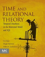
Here’s a simple example (the query is “For each supplier, get full supplier information, together with a TRIPLE value that’s equal to three times the supplier’s status”):
EXTEND S : { TRIPLE := 3 * STATUS }
Here’s the result:
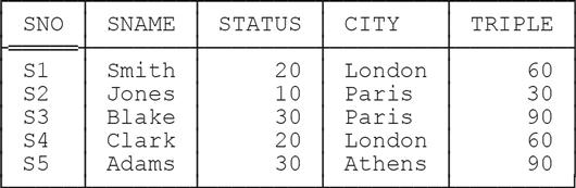
The second form of EXTEND differs from the first only in that the target attribute, in the attribute assignment in braces, isn’t a “new” attribute as it is in the first form—instead, it’s an attribute that already exists in the relation that’s being extended. For example:
EXTEND S : { STATUS := 3 * STATUS }Here’s the result:
For completeness, here’s the definition:
Definition: Let relation r have an attribute called A. Then the expression EXTEND r : {A := exp} denotes an extension of r, and it returns the relation with heading the same as that of r and body the set of all tuples t such that t is derived from a tuple of r by replacing the value of A by a value that’s computed by evaluating the expression exp on that tuple of r.6
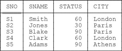
As a matter of user convenience, Tutorial D also supports a multiple form of EXTEND, which allows several attribute assignments to be done in parallel (“simultaneously”). For example:
EXTEND S : { TRIPLE := 3 * STATUS , STATUS := STATUS + 5 , CITY := 'Oslo' }Here’s the result:
Image Relations
An image relation is, loosely, the “image” within some relation r of some tuple (usually but not necessarily a tuple within some distinct relation r') For example, given our usual suppliers-and-shipments database, the following is the image within the shipments relation of the tuple in the suppliers relation for supplier S4:
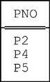
Clearly, this particular image relation can be obtained by evaluating the following expression (a projection of a restriction):
( SP WHERE SNO = SNO ( 'S4' ) ) { PNO }But image relations in general are such a useful and widely applicable concept that it’s desirable to define a shorthand for them, and so we do. Here’s an example to illustrate:
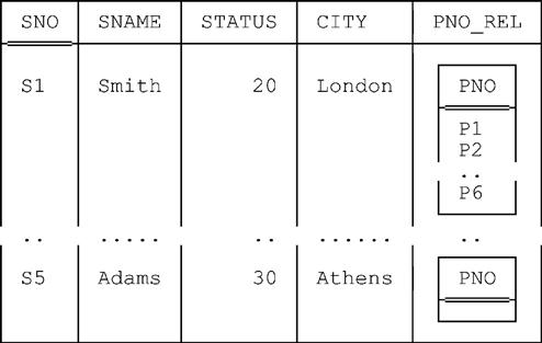
EXTEND S : { PNO_REL := !!SP }In this expression, the subexpression !!SP—pronounced “bang bang SP” or “double bang SP”—is an image relation reference, and it denotes the image relation within SP corresponding to “the current tuple” of S (i.e., it denotes that restriction of SP having the same values for common attributes as that current tuple, projected over all but those common attributes).7 Thus, the foregoing expression is evaluated as follows:
■ The expression overall (EXTEND S …) denotes a certain extension of the suppliers relation. You can imagine that extension being done a tuple at a time in some arbitrary sequence. Consider one such tuple, say the tuple for supplier Sx. For that tuple, then, the expression !!SP denotes the corresponding image relation within the shipments relation. For example, if Sx is S4, it denotes the relation shown at the beginning of this section.
■ So the new attribute PNO_REL is relation valued—recall from Chapter 1 that relation valued attributes are certainly legal—and the value for that attribute for supplier Sx is precisely the corresponding image relation.
Here’s the overall result (in outline):
Group and Ungroup
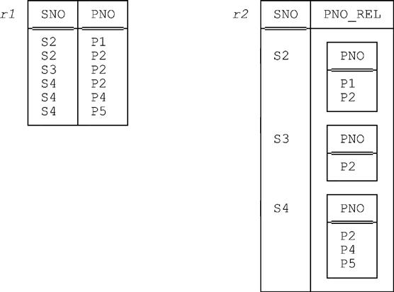
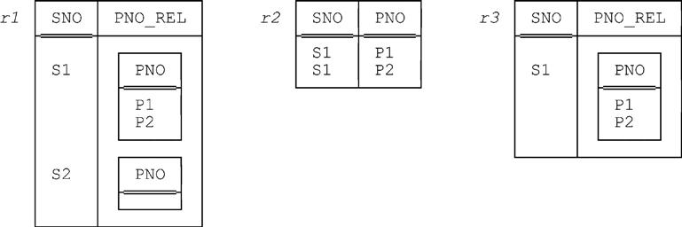
To repeat, relation valued attributes (RVAs for short) are certainly legal. So consider Fig. 2.1, which shows (a) a relation r1 without any RVAs—it’s a simplified version of our usual shipments relation—and (b) another relation r2 that does have an RVA. Observe that relations r1 and r2 are clearly not the same as one another but that, equally clearly, they do both represent the same information.
Here are the corresponding predicates:
r1: Supplier SNO is able to supply part PNO.
r2: Supplier SNO is able to supply part p, if and only if p appears as a PNO value in some tuple in the body of relation PNO_REL.8
And here for the record are the corresponding types:
r1: RELATION { SNO SNO , PNO PNO }
r2: RELATION { SNO SNO , PNO_REL RELATION { PNO PNO } }
Now, we obviously need a way to map between relations without RVAs (like r1) and corresponding relations with them (like r2), and that’s the purpose of the GROUP and UNGROUP operators. For example, given relations r1 and r2 from Fig. 2.1, the expression
r1 GROUP { PNO } AS PNO_RELeffectively maps r1 to r2; likewise, the expression
r2 UNGROUP PNO_REL
effectively maps r2 to r1.
In order to define the GROUP and UNGROUP operators more formally, it’s convenient first to introduce two auxiliary operators called WRAP and UNWRAP. Basically, WRAP wraps up specified attributes of a given relation into a single attribute that’s tuple valued, and UNWRAP does the opposite. For example, given relation r1 from Fig. 2.1, the expression
r1 WRAP { PNO } AS PNO_TUPproduces the relation r3 shown in Fig. 2.2, and then the expression
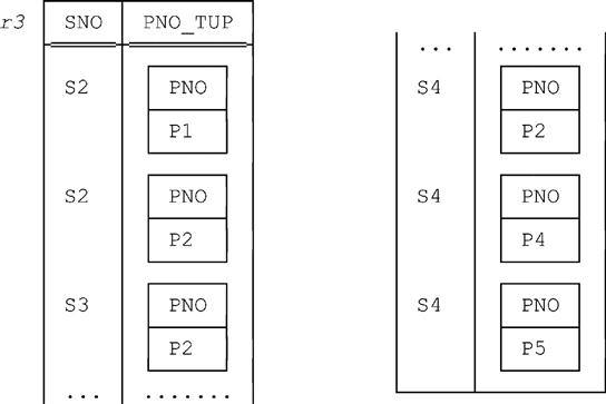
r3 UNWRAP PNO_TUP
produces relation r1 again. (Please note that the PNO_TUP values in relation r3 are tuples, not relations—PNO_TUP is a tuple valued attribute, not a relation valued attribute.)
Here now are definitions of these various operators. Note: We give these definitions mainly for completeness; they might be a little difficult to understand, at least on a first reading.
Definition: Let relation r have attributes called A1,A2, …, Am, B1, B2, …, Bn (only), and let BT be an attribute name that’s distinct from that of every attribute Ai (1 ≤ i ≤ m). Then the expression r WRAP {B1,B2, …,Bn} AS BT denotes the wrapping of r on {B1,B2, …,Bn}, and it returns the relation denoted by the expression (EXTEND r : {BT := TUPLE {B1 B1, B2 B2, …, Bn Bn}}){A1,A2, …,Am,BT}.
Definition: Let relation r have attributes called A1, A2, …, Am, and BT (only), and let attribute BT be tuple valued and have attributes called B1, B2, …, Bn (only); further, let no Ai have the same name as any Bj (1 ≤ i ≤ m, 1 ≤ j ≤ n). Then the expression r UNWRAP BT denotes the unwrapping of r on BT, and it returns the relation denoted by the expression (EXTEND r : {B1 := B1 FROM BT, B2 := B2 FROM BT, …, Bn := Bn FROM BT}){ALL BUT BT}.
Note: This latter definition makes use of expressions of the form X FROM tx, where X is an attribute name and tx is a tuple expression. Such an expression is, of course, defined to return the value of attribute X from the tuple denoted by tx.9
Definition: Let the heading of relation r be partitioned into subsets A = {A1,A2, …,Am} and B = {B1,B2 …,Bn}; also, let BR be an attribute name that’s distinct from that of every attribute Ai (1 ≤ i ≤ m). Then the expression r GROUP {B1,B2, …,Bn} AS BR denotes the grouping of r on {B1,B2, …,Bn}, and it returns a relation s with heading{A1,A2, …,Am,BR}, where BR is a relation valued attribute with heading {B1,B2, …,Bn}. The body of s is defined as follows. Let x be the result of r WRAP {B1,B2, …,Bn} AS BT. For each distinct A value a in x, let br be the relation whose tuples are all and only those BT values from tuples in x in which the A value is a; let t be a tuple with heading {A1,A2, …,Am,BR} with A value a and BR value br; then, and only then, t is a tuple of s.
Definition: Let relation s have a relation valued attribute BR with heading {B1,B2, …,Bn}, and let A = {A1,A2, …,Am} be all of the attributes of s other than BR; also, let no Ai have the same name as any Bj (1 ≤ i ≤ m, 1 ≤ j ≤ n). Then the expression s UNGROUP BR denotes the ungrouping of s on BR, and it returns a relation r with heading {A1,A2, …,Am, B1,B2, …,Bn}. The body of r is defined as follows. Let x be a relation with heading {A1,A2, …Am,BT}, where BT is a tuple valued attribute with heading {B1,B2, …,Bn}, and body defined as follows: For each tuple of s, x contains one tuple (t, say) for each tuple in the BR value in that s tuple; each such tuple t contains an A value equal to the A value from the s tuple in question and a BT value equal to some tuple from the BR value in the s tuple in question. Let x contain no other tuples. Then r is the result of x UNWRAP BT.
Note, incidentally, that given some relation r and some grouping of r, there’s always an inverse ungrouping that yields r again; however, the converse isn’t necessarily so. The following example illustrates the point. Consider the relation—call it r1—shown on the left in Fig. 2.3, and note in particular that the PNO_REL value in that relation for supplier S2 is empty. The expression r1 UNGROUP PNO_REL yields the relation r2 shown in the middle of the figure. And the expression r2 GROUP {PNO} AS PNO_REL then yields the relation r3 shown on the right, which is obviously not the same as the original relation r1.
Note: Refer again to Fig. 2.1. Here again is the expression that derives relation r2 from relation r1:
r1 GROUP { PNO } AS PNO_RELAs you might have realized, the following expression will produce exactly the same result:
EXTEND r1 { SNO } : { PNO_REL := !!r1 }Indeed, as this example suggests, GROUP can actually be defined in terms of EXTEND and image relations. What’s more, the same goes for UNGROUP as well. We choose not to show those definitions here, but you can find them if you’re interested in reference [46]. Of course, we’re not suggesting we get rid of our useful GROUP and UNGROUP operators—but it’s at least interesting, and perhaps pedagogically helpful, to note that the semantics of GROUP and UNGROUP can in fact be explained in such a manner.
Extend bis
EXTEND and image relations can be used together to perform summarizations. Here’s an example (the query is “For each supplier, get the supplier number and a count of the number of parts that supplier supplies”):
EXTEND S { SNO } : { PCT := COUNT ( !!SP ) }Here’s the result:
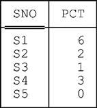
■ COUNT here is an aggregate operator. In general, an aggregate operator is an operator that derives a single value from the “aggregate”—i.e., the set or bag10—of values of some attribute of some relation (or, in the case of COUNT, which is slightly special, from the “aggregate” that’s the entire relation). Typical aggregate operators include COUNT, SUM, AVG, MAX, MIN, AND, and OR (where SUM and AVG apply only to aggregates of numeric values; MAX and MIN apply only to aggregates of values for which the operators “>” and “<” are defined; and AND and OR apply only to aggregates of boolean values).
■ As already indicated, the expression overall in the example—i.e., the EXTEND invocation—denotes a certain summarization. Loosely, to perform a summarization on some given relation r means, for each tuple of r, (a) to identify some corresponding image relation, and then (b) to perform some aggregation over that image relation—which is, of course, exactly what we did in the example.
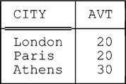
Here’s another example (note the syntax of the AVG invocation in particular):
EXTEND S { CITY } : { AVT := AVG ( !!S , STATUS ) }Result:
Tutorial D also allows aggregate operator invocations to appear in WHERE conditions, as in the following example (the query is “Get suppliers able to supply two or more distinct parts”):
S WHERE COUNT ( !!SP ) > 1
Note: This expression isn’t a proper relational restriction as such because the boolean expression (i.e., the WHERE condition) isn’t a restriction condition as such. However, the expression overall can be regarded as shorthand for the following:
( ( EXTEND S : { x := COUNT ( !!SP ) } WHERE x > 1 ) { ALL BUT x }And the boolean expression (i.e., the WHERE condition) in this latter formulation is a proper restriction condition, of course.
Relational Comparisons
As noted in Chapter 1, the “=” comparison operator is—in fact, must be—defined for every type, and relation types are no exception to this rule. That is, given two relations r1 and r2 of the same type T, we must certainly be able to test whether they’re equal. For example:
S { SNO } = SP { SNO }The left comparand here is the projection of suppliers on SNO, the right comparand is the projection of shipments on SNO, and the comparison gives TRUE if these two projections are equal, FALSE otherwise. (Given our usual sample values, it gives FALSE, of course.)
The comparison operators “≠”, “⊆” (is included in), “⊂” (is properly included in), “⊇” (includes), and “⊃” (properly includes) should obviously all be supported as well. Here’s another example, illustrating the use of “⊃”:
S { SNO } ⊃ SP { SNO }The meaning of this expression, considerably paraphrased, is: “Some suppliers supply no parts at all” (which, please note, does necessarily evaluate to either TRUE or FALSE).
Aside: There’s a tiny technical issue here that might be bothering you. The operators of the relational algebra are supposed to form a closed system, in the sense that the result of every such operator is supposed to be a relation. But the result of the relational comparison operators is, of course, not a relation but a truth value. Thus, it’s not clear that these operators should be considered part of the algebra as such (writers differ on this issue). However, the important point as far as we’re concerned is simply that the operators are certainly available, regardless of whether we consider them part of the algebra as such. End of aside.
Here now is an example of the use of a relational comparison in formulating a fairly complicated (but realistic) query:
S WHERE ( MSP ) { PNO } ⊇ ( SP WHERE SNO = SNO ( 'S2' ) ) { PNO }The query is “Get supplier information for suppliers who supply all parts supplied by supplier S2.”
One very common requirement is to be able to perform an “=” comparison between some given relation r and the corresponding empty relation (i.e., the unique empty relation of the same type as r)—in other words, a test to see whether r is empty. So we define a shorthand:
IS_EMPTY ( r )
This expression is defined to return TRUE if r is empty and FALSE otherwise. It can be regarded as shorthand for the following:
r = ( r WHERE FALSE )
(It’s also equivalent to r{ } = TABLE_DUM.) The inverse operator is useful too:
IS_NOT_EMPTY ( r )
This expression is equivalent to NOT (IS_EMPTY(r)), or r{ } = TABLE_DEE.
Formulating Expressions One Step at a Time
Consider the following expression (the query is “Get pairs of supplier numbers such that the suppliers concerned are in the same city”):
( ( ( S RENAME { SNO AS XNO } ) { XNO , CITY } JOIN ( S RENAME { SNO AS YNO } ) { YNO , CITY } ) WHERE XNO < YNO ) { XNO, YNO }The result has two “supplier number” attributes, called XNO and YNO. Note: The purpose of the condition XNO < YNO is twofold—it eliminates pairs of supplier numbers of the form (x,x), and it guarantees that the pairs (x,y) and (y,x) won’t both appear. Of course, we’re assuming here that the operator “<” has been defined in connection with type SNO.
We now show another formulation of the query in order to show how Tutorial D’s WITH construct can be used to simplify the business of formulating what might otherwise be considered rather complicated expressions:
WITH ( t1 := ( S RENAME { SNO AS XNO } ) { XNO , CITY } , t2 := ( S RENAME { SNO AS YNO } ) { YNO , CITY } ,t3 := t1 JOIN t2,
t4 := t3 WHERE XNO < YNO ) :
t4 { XNO , YNO }WITH isn’t an operator as such, it’s just a syntactic device that lets us introduce names for subexpressions and thereby lets us see the trees as well as the forest (as it were). As the example suggests, a WITH specification consists of the keyword WITH followed by a parenthesized commalist of assignments of the form name := expression, that parenthesized commalist then being followed by a colon. For each such assignment, the specified expression is evaluated and the result is effectively assigned to a temporary variable with the specified name. Also, since the assignments are effectively performed in sequence as written, any given assignment is allowed to refer to names introduced earlier within the same commalist.
Note: Tutorial D allows WITH specifications on statements as well as on expressions. Here’s a simple example (the statement here is a relational assignment statement—see Chapter 3 for further explanation):
WITH ( X := RELATION { TUPLE { SNO SNO ( 'S5' ), PNO PNO ( 'P6' ) } } ) : SP := SP UNION X ;Relational Completeness
We began this chapter by saying the set of algebraic operators was open ended. That’s true, but what we didn’t say was that the operators in question, taken together, are supposed to be at least relationally complete [22]. Relational completeness is a basic measure of the expressive capability of a language. If a language is relationally complete, then it means—speaking very loosely, please note!—that queries of arbitrary complexity can be formulated in that language without having to resort to branching or iterative loops. And in order to be relationally complete, it’s sufficient that the language in question support, directly or indirectly, all of the following operators: restriction, projection, JOIN, UNION, NOT MATCHING, and EXTEND (first version), together with the relational inclusion operator “⊆”
Exercises
2.1 Write algebraic expressions for the following queries:
b. Get supplier numbers for suppliers able to supply part P1.
c. Get part numbers for parts capable of being supplied by a supplier in London.
d. Get part numbers for parts capable of being supplied, but not by a supplier in London.
e. Get part numbers for parts capable of being supplied by either a supplier in London or a supplier in Paris or both.
f. Get pairs of part numbers such that some supplier is able to supply both of the indicated parts.
g. For each supplier in Paris, get the supplier number and the total number of parts capable of being supplied by the supplier in question.
h. Get supplier numbers for suppliers with a status lower than that of supplier S1.
i. Get supplier numbers for suppliers whose city is first in the alphabetic list of such cities.
j. Get part numbers for parts capable of being supplied by all suppliers in London.
k. Get supplier number / part number pairs such that the indicated supplier is unable to supply the indicated part.
l. Get pairs of supplier numbers for suppliers who are able to supply exactly the same set of parts each.
2.2 Consider the following definitions for the relvars in a courses-and-students database:11
VAR COURSE BASE RELATION
{ COURSENO COURSENO , CNAME NAME , AVAILABLE DATE }
KEY { COURSENO } ;
VAR STUDENT BASE RELATION
{ STUDENTNO STUDENTNO , SNAME NAME , REGISTERED DATE }
KEY { STUDENTNO } ;
VAR ENROLLMENT BASE RELATION
{ COURSENO COURSENO , STUDENTNO STUDENTNO , ENROLLED DATE }
KEY { COURSENO , STUDENTNO }
FOREIGN KEY { COURSENO } REFERENCES COURSE
FOREIGN KEY { STUDENTNO } REFERENCES STUDENT ;
Types COURSENO and STUDENTNO are user defined, type DATE is built in. You can assume these types each have an associated selector operator with the same name, each one taking a single argument of type CHAR and returning a value of the appropriate type. The predicates for the relvars are as follows:
■ COURSE: Course COURSENO, named CNAME, became available at the university on date AVAILABLE.
■ STUDENT: Student STUDENTNO, named SNAME, registered with the university on date REGISTERED.
■ ENROLLMENT: Student STUDENTNO enrolled on course COURSENO on date ENROLLED.
a. Write a query to get student number and name for students who are enrolled on all the courses student ST2 is enrolled on.
b. Consider the following expression:
( ( STUDENT WHERE STUDENTNO = STUDENTNO ( 'ST1' ) ) JOIN COURSE ) WHERE AVAILABLE > REGISTERED
Write a predicate for the relation denoted by this expression.
Answers
2.1 The following solutions aren’t the only ones possible. Note: This remark applies to many of the solutions provided in this book; we won’t bother to keep repeating it, however, letting this one disclaimer do duty for all.
b. ( SP WHERE PNO = PNO ( 'P1' ) ) { SNO }
c. ( SP MATCHING ( S WHERE CITY = 'London' ) ){ PNO }
d. ( SP NOT MATCHING ( S WHERE CITY = 'London' ) ) { PNO }
e. ( SP MATCHING ( S WHERE CITY = 'London' OR CITY = 'Paris') ) { PNO }
f. ( JOIN { SP RENAME { PNO AS XNO } , SP RENAME { PNO AS YNO } } ) { XNO , YNO }
g. EXTEND ( S WHERE CITY = 'Paris' ) { SNO } : { PCT := COUNT ( !!SP ) }
h. ( S WHERE STATUS < STATUS FROM ( TUPLE FROM ( S WHERE SNO = SNO ( 'S1' ) ) ) ) { SNO }
i. ( S WHERE CITY = MIN ( S , CITY ) ) { SNO }
j. ( P WHERE !!SP { SNO } ⊇ ( S WHERE CITY = 'London' ) { SNO } ) { PNO }
k. ( S { SNO } JOIN SP { PNO } ) MINUS SP
l. ( ( ( ( SP GROUP { PNO } AS X } ) RENAME { SNO AS XNO } ) JOIN
( ( SP GROUP { PNO } AS X } ) RENAME { SNO AS YNO } ) ) ) { XNO , YNO }
a. ( STUDENT WHERE ( !!ENROLLMENT ) { COURSENO } ⊇
( ENROLLMENT WHERE STUDENTNO = STUDENTNO ( 'ST2' ) ) { COURSENO } ) { STUDENTNO , SNAME }
b. Predicate: Student STUDENTNO has student number ST1, is named SNAME, and registered on date REGISTERED; course COURSENO is named CNAME and became available on date AVAILABLE; and AVAILABLE is more recent than REGISTERED.
Note: What this exercise illustrates is the following. Recall from Chapter 1 that every relation does have a predicate. Well, the predicate for the relation denoted by some operational expression can be obtained from the predicates for the operands (relations) involved in that expression, together with the semantics of the operators involved in that expression. For example, if relations r1 and r2 have predicates p1 and p2, respectively, then the relation denoted by r1 JOIN r2 has predicate p1 AND p2. For further discussion of such matters, see, e.g., reference [28].