Types and Relations
This chapter is the first of three devoted to reviewing the basics of relational theory. It explains relations as such, as well as the supporting notion of types (aka domains), in considerable depth. With regard to types; it discusses values, variables, operators, parameters, arguments, expressions, and polymorphism; equality and assignment; system defined vs. user defined types; scalar vs. nonscalar types; possible vs. physical representations; type generators and generated vs. nongenerated types; type constraints; and selectors, literals, and THE_ operators. With regard to relations, it discusses tuples, attributes, and relation headings and bodies; relation and tuple types; TABLE_DEE and TABLE_DUM; relation valued attributes; predicates and propositions; and The Closed World Assumption. The chapter also introduces the running example (i.e., the suppliers-and shipments-database).
Keywords
domain; relation; tuple; attribute; relation heading; relation body; type theory; relation predicate; The Closed World Assumption
What type of relation do you mean?
—Anon.:
Where Bugs Go
The relational model is, of course, defined in terms of relations, and relations in turn are defined in terms of types. This first chapter explains these two constructs in detail. First, however, it introduces the running example.
The Running Example
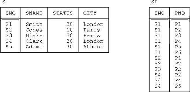
Most of the examples in this book are based on the well known suppliers-and-parts database—or, more precisely, on a simplified version of that database that we refer to as suppliers and shipments. Fig. 1.1 shows a set of sample values for that simplified database (and please note that we’ll be assuming those specific sample values in examples throughout this part of the book, barring explicit statements to the contrary). Note: In case you happen to be familiar with the more usual version of this database as discussed in, e.g., reference [45], we explain here briefly what the simplifications consist of:
■ First of all, we’ve dropped the parts relvar P entirely (hence the revised name “suppliers and shipments”). Note: The term relvar is short for relation variable. Relation variables are discussed in detail in Chapter 3.
■ Second, we’ve removed attribute QTY (“quantity”) from the shipments relvar SP, leaving just attributes SNO and PNO.
■ Third, we (re)interpret that revised SP relvar thus: “Supplier SNO is currently able to supply part PNO. ” In other words, instead of standing for actual shipments of parts by suppliers, as it did in, e.g., reference [45], relvar SP now stands for what might be called potential shipments—i.e., the ability of certain suppliers to supply certain parts.
Overall, then, the database is meant to be interpreted as follows:
■ Relvar S represents suppliers under contract. Each such supplier has a supplier number (SNO), unique to that supplier; a supplier name (SNAME), not necessarily unique (though the sample SNAME values shown in Fig. 1.1 do happen to be unique); a status or rating value (STATUS); and a location (CITY). Note: In the rest of this book we’ll refer to “suppliers under contract,” most of the time, as just suppliers for short.
■ Relvar SP represents potential shipments—it shows which suppliers are capable of supplying, or shipping, which parts. Obviously, the combination of SNO and PNO values for a given “potential shipment” is unique to that shipment. Note: In the rest of this book we’ll take the liberty of referring to “potential shipments”—somewhat inaccurately, but very conveniently—as just shipments for short. Also, we’ll assume it’s possible for a given supplier to be under contract at some time and yet not actually be able to supply any parts at that time (supplier S5 is a case in point, given the sample values of Fig. 1.1).
Here for purposes of reference are formal definitions for the example, expressed in a language called Tutorial D—or, rather, in a version of that language that’s been tailored slightly in order to suit the purposes of this book. Tutorial D is a computationally complete programming language with fully integrated database functionality and, we believe, more or less self-explanatory syntax. It was introduced in the first (1998) edition of reference [52] as a vehicle for teaching database concepts. All coding examples in this book are expressed in that language or certain specified extensions thereto (except, of course, for the SQL-specific examples in Part IV).
TYPE SNO … ;
TYPE PNO … ;
TYPE NAME … ;
VAR S BASE
RELATION
{ SNO SNO , SNAME NAME, STATUS INTEGER , CITY CHAR } KEY { SNO } ;VAR SP BASE
RELATION
{ SNO SNO , PNO PNO } KEY { SNO , PNO } FOREIGN KEY { SNO } REFERENCES S ;To elaborate briefly (note, however, that all of the technical issues illustrated by this example and discussed in outline below will be explained in more detail either later in this chapter or somewhere in the next two):
■ The first three lines are type definitions (shown here in outline only; further details are given in the section “Types,” immediately following the present section). The specified types—SNO, PNO, and NAME—are user defined types, and they’re used in the definitions of attributes SNO and SNAME in relvar S and attributes SNO and PNO in relvar SP. By contrast, attributes STATUS and CITY in relvar S are of system defined types—namely, INTEGER (integers) and CHAR (character strings of arbitrary length), respectively—and, of course, no explicit type definitions are needed for such types. Note: In what follows, we’ll assume the availability of another system defined type also: namely, type BOOLEAN (truth values), consisting of just the two values TRUE and FALSE.
■ The next seven lines constitute the definition of relvar S. The keyword VAR indicates that the statement overall defines a variable. The variable in question is called S. The keyword BASE indicates the kind of variable being defined; it stands for “base relvar,” which is the kind of relvar S is. Note: Relvars come in several different varieties, of which the most important are (a) base, or real, relvars and (b) virtual relvars, also called views. In this book, however, we’ll have little to say regarding virtual relvars until we get to Chapter 15; prior to that point, therefore, we’ll adopt the simplifying assumption that the unqualified term relvar always means a base relvar specifically, unless the context demands otherwise.
■ Within the definition for relvar S, lines 2–6 specify the type of the variable being defined. The keyword RELATION shows it’s a relation type, and the next four lines specify the corresponding attributes, where each attribute consists of the applicable attribute name together with the name of the corresponding type. The complete set of attribute specifications is enclosed in braces. No significance attaches to the order in which the attributes are specified within those braces. Note: For a general explanation of how braces are used in Tutorial D, please see Appendix D.
■ Line 7 of the definition for relvar S defines {SNO} to be a key for that relvar.
■ The last six lines constitute the definition of relvar SP. The definition follows the same general pattern as that for relvar S; the only new construct is the foreign key specification in the last line, which defines {SNO} to be a foreign key in relvar SP referencing the “target” key {SNO} in relvar S. Note, incidentally, that relvar SP is “all key.”
Types
Relations in the relational model are defined over types (also known as domains—the terms are interchangeable, but we’ll stay with types). Types are discussed in the present section, relations are discussed in the next.
What exactly is a type? Among other things, it’s a set of values. Examples include:
■ The set of all integers (type INTEGER)
■ The set of all character strings (type CHAR)
■ The set of all supplier numbers (type SNO)
Aside: Instead of saying that (e.g.) type INTEGER is the set of all integers, it would be more correct to say it’s the set of all integers that are capable of representation in the computer system under consideration. Obviously there’ll be some integers that are beyond the representational capability of any given system. In what follows, however, we won’t usually bother to be quite so precise. End of aside.
Every value has, or is of, some type; in fact, every value is of exactly one type.1 Moreover:
■ Every variable is defined, or “declared,” to be of some type, meaning that every possible value of the variable in question is a value of the type in question.
■ Every attribute of every relation is declared to be of some type, meaning that every possible value of the attribute in question is a value of the type in question.
■ Every operator that returns a result is declared to be of some type, meaning that every possible result that can be returned by an invocation of the operator in question is a value of the type in question. Note: An operator that returns a result is called a read-only operator; an operator that returns no result but updates one or more of its arguments instead is called an update operator. Examples of both kinds are given in the subsection “User Defined Operators” later in this section. Further, let Op be an update operator. Since an invocation of Op doesn’t denote a value, Op doesn’t have a declared type (though its parameters do—see the bullet item immediately following).
■ Every parameter of every operator is declared to be of some type, meaning that every possible argument that can be substituted for the parameter in question is a value or variable of the type in question. Note that it must be a variable if the operator in question is an update operator and the argument corresponding to the parameter in question will be updated by an invocation of the operator in question.
■ More generally, every expression is declared to be of some type—namely, the type declared for the outermost operator (necessarily a read-only operator) involved in the expression in question, or equivalently the type of the value denoted by that expression.
Aside: The remarks concerning operators and parameters in the two bullet items immediately preceding require some slight refinement if the operator in question is polymorphic. An operator is said to be polymorphic if it’s defined in terms of some parameter P and the argument corresponding to P can be of different types on different invocations. The equality operator “=” is an obvious example: We can compare values of any type for equality (just so long as the values in question are both of the same type), and so “=” is polymorphic—it applies to integers, and character strings, and supplier numbers, and in fact to values of every type. Analogous remarks apply to the assignment operator “:=”; indeed, we follow reference [49] in requiring both “=” and “:=” to be defined for every type. Further examples of polymorphic operators include aggregate operators such as SUM and MAX (see Chapter 2); operators of the relational algebra such as UNION and JOIN (again, see Chapter 2); and the operators defined for intervals in Part II of this book. End of aside.
Any given type is either system defined or user defined2 As previously noted, of the types mentioned in connection with the running example, types INTEGER, CHAR, and BOOLEAN are system defined (or so we assume for the purposes of this book, at any rate), and types SNO, NAME, and PNO are user defined.
Next, any type whatsoever, regardless of whether it’s system or user defined, can be used as the basis for defining variables, attributes, operators, and parameters. Well … there are two small exceptions to this statement, both of them having to do with attribute types specifically:
■ First, the relational model expressly prohibits relations in the database from having attributes of any pointer type—meaning in particular, albeit a little loosely, that no relation in the database is allowed to have an attribute whose values are pointers to tuples in the database. Note: Relations and tuples are discussed in the next section.
■ The second limitation is a little harder to state, but what it boils down to is this: If relation r has heading H, then no attribute of r can be defined in terms of a relation or tuple type that has that same heading H, at any level of nesting. Note: Headings too are discussed in the next section.
Next, it’s usual to think of types, informally, as being either scalar or nonscalar. Loosely, a type is scalar if it has no user visible components and nonscalar otherwise—and values, variables, attributes, operators, parameters, and expressions of some type T are scalar or nonscalar according as type T itself is scalar or nonscalar. For example:
■ Type INTEGER is a scalar type (it has no user visible components); hence, values, variables, and so on of type INTEGER are also all scalar.
■ Relation and tuple types are nonscalar (the pertinent user visible components being the corresponding attributes); hence, relation and tuple values, variables, and so on are also all nonscalar.
That said, we must emphasize that these notions are quite informal. In particular, the relational model nowhere relies on the scalar vs. nonscalar distinction in any formal sense. In this book, however, we do appeal to it informally from time to time, because we do find it at least intuitively useful.3 To be specific, we use the term scalar in connection with types that are neither tuple nor relation types, and the term nonscalar in connection with types that are either tuple or relation types.4
Aside: Another term you’ll sometimes hear used to mean “scalar” is encapsulated. Be aware, however, that this term is also used—especially in object oriented contexts—to refer to the physical bundling, or packaging, of code and data (or operator definitions and data representation definitions, to be more precise about the matter). But to use the term in this latter sense is to mix model and implementation considerations; clearly the user shouldn’t care, and shouldn’t need to care, whether code and data are physically bundled together or are kept separate. See reference [36] for further discussion. End of aside.
Following on from the foregoing, we need to explain that although scalar types have no user visible components, they do have what are called possible representations (“possreps” for short), and those possible representations are user visible and do have user visible components, as we’ll see in a moment. Don’t be misled, however: Those user visible components aren’t components of the type, they’re components of the possrep. The type itself is still scalar in the sense explained above.
By way of illustration, suppose we have a user defined scalar type called QTY (“quantity”). Assume for the sake of the example that a possible representation called QPR is declared for this type that says, in effect, that quantities can “possibly be represented” by positive integers, as indicated here:
TYPE QTY POSSREP QPR { Q INTEGER CONSTRAINT Q ≥ 1 … } ;Then the specified possrep certainly does have user visible components—in fact, it has exactly one such component, Q, of type INTEGER—but, to repeat, quantities per se do not.
Here’s a more complicated example that illustrates the same point:
TYPE POINT /* geometric points in two-dimensional space */
POSSREP CARTESIAN { X RATIONAL, Y RATIONAL … } POSSREP POLAR { RHO RATIONAL, THETA RATIONAL … } ;Type POINT has two distinct possreps, CARTESIAN and POLAR, reflecting the fact that points in two-dimensional space can indeed “possibly be represented” by either cartesian or polar coordinates. Each of those possreps in turn has two components, both of which are of type RATIONAL (“rational numbers”).5 Note carefully, however, that, to say it again, type POINT per se is still scalar—it has no user visible components. Note too that the physical representation of POINT values, in the particular implementation at hand, might be cartesian coordinates, or it might be polar coordinates, or it might be something else entirely. In other words, possible representations (which are, to repeat, user visible) are indeed only possible ones; physical representations are an implementation matter merely and should never be visible to the user.
Next, be aware that each POSSREP specification causes automatic definition of the following more or less self-explanatory operators:
■ One selector operator, which allows the user to select, or specify, a value of the type in question by supplying a value for each component of the possible representation in question
■ A set of THE_ operators (one such for each component of the possible representation in question), which allow the user to access components of the corresponding possible representation of values of the type in question
Aside: When we say a POSSREP specification causes “automatic definition” of such operators, what we mean is this: Whatever agency—possibly the system, possibly some human user—is responsible for implementing the type in question is also responsible for implementing those operators; moreover, until those operators have been implemented, the process of implementing the type can’t be regarded as complete. End of aside.
We adopt certain naming conventions in connection with the foregoing operators. To be specific, we adopt the conventions that (a) selectors have the same name as the corresponding possrep, and (b) THE_ operators have names of the form THE_C, where C is the name of the corresponding component of the corresponding possrep. Thus, type QTY has one selector, called QPR, and one THE_ operator, called THE_Q. By contrast, type POINT has two selectors, called CARTESIAN and POLAR; it also has two THE_ operators corresponding to the CARTESIAN possrep, called THE_X and THE_Y, and two THE_ operators corresponding to the POLAR possrep, called THE_RHO and THE_THETA. Here are some sample invocations:
QPR ( 250 )
/* returns the quantity corresponding to the integer 250 */
THE_Q ( QX )
/* returns the integer corresponding to the quantity */
/* value in QX, where QX is a variable of type QTY */
CARTESIAN ( 5.0 , −2.5 )
/* returns the point with x = 5.0 and y = −2.5 */
CARTESIAN ( X1 , Y1 )
/* returns the point with x = X1 and y = Y1 , where X1 and */
/* Y1 are variables of type RATIONAL */
POLAR ( 1.7 , 2.0 )
/* returns the point with rho = 1.7 and theta = 2.0 */
THE_X ( P )
/* returns the x coordinate of the point value in P, */
/* where P is a variable of type POINT */
THE_RHO ( P )
/* returns the rho coordinate of the point value in P, */
/* where P is a variable of type POINT */
THE_Y ( exp )
/* returns the y coordinate of the point denoted by the */
/* expression exp (which must be of type POINT) */
We adopt another naming convention also: If type T has a possrep with no explicitly declared name, then that possrep is named T by default. By way of example, we could simplify the definition of type QTY by omitting the possrep name QPR, thus:
TYPE QTY POSSREP { Q INTEGER CONSTRAINT Q ≥ 1 … } ;And then we could simplify the first selector invocation in the foregoing list of examples to the following more user friendly form:
QTY ( 250 )
/* returns the quantity corresponding to the integer 250 */
Note: As several of the foregoing examples should be sufficient to suggest, selectors—or selector invocations, rather—are a generalization of the more familiar concept of a literal.6 In fact, all literals are selector invocations; however, not all selector invocations are literals. To be specific, a selector invocation is a literal if and only if its argument expressions are all literals in turn. Thus, of the selector invocations shown above, QTY (250) (or QPR (250)), CARTESIAN (5.0,−2.5), and POLAR (1.7,2.0) are literals and the others aren’t.
User Defined Operators
The foregoing discussion of THE_ operators in particular touches on another crucial issue: namely, the fact that the type concept includes the associated notion of the operators that apply to values and variables of the type in question. (By definition, values and variables of a given type can be operated upon only by means of the operators defined in connection with that type.) For example, in the case of the system defined type INTEGER:
■ The system defines operators “:=”, “=”, “>”, and so on, for assigning and comparing integers.
■ It also defines operators “+”, “*”, and so on, for performing arithmetic on integers.
■ It does not define operators “| |” (concatenate), SUBSTR (substring), and so on, for performing string operations on integers. In other words, string operations on integers aren’t supported.
By way of another example, consider the user defined type SNO. Then whoever actually defines that type will certainly define “:=” and “=” operators, and perhaps “>” and “<” operators as well, for assigning and comparing supplier numbers. However, that user will probably not define operators “+”, “*”, and so on, which means that arithmetic on supplier numbers won’t be supported.
We see, therefore, that users will necessarily have the ability to define their own operators. This fact isn’t particularly relevant to the primary topic of the present book—at least, it won’t be until we get to Chapter 18—but we show a few examples here in order to give some idea as to what such a feature might look like. First, here’s the definition for a user defined operator called ABS (“absolute value”) for the system defined type INTEGER:
OPERATOR ABS ( I INTEGER ) RETURNS INTEGER ;
RETURN ( IF I ≥ 0 THEN +I ELSE −I END IF ) ;
END OPERATOR ;
This operator is declared to be of type INTEGER (i.e., it returns an integer when it’s invoked), and it has just one parameter, I, which is also of declared type INTEGER.
By way of a second example, here’s the definition for an operator DIST (“distance between”) for the user defined type POINT:
OPERATOR DIST ( P1 POINT , P2 POINT ) RETURNS RATIONAL ;
RETURN ( SQRT ( ( THE_X ( P1 ) − THE_X ( P2 ) ) ↑ 2 + ( THE_Y ( P1 ) − THE_Y ( P2 ) ) ↑ 2 ) ) ;
END OPERATOR ;
This operator is of declared type RATIONAL; it has two parameters, P1 and P2, both of declared type POINT. (We’re assuming for the sake of the example that the operator SQRT returns a rational number result, representing the nonnegative square root of its nonnegative rational number argument. The symbol “↑” means “raise to the power of.”)
Now, ABS and DIST are both read-only operators. Here by contrast is an example of a definition for an update operator called REFLECT:
OPERATOR REFLECT ( P POINT ) UPDATES { P } ;
THE_X ( P ) := − THE_X ( P ),
THE_Y ( P ) := − THE_Y ( P ) ;
END OPERATOR ;
This operator has just one parameter P, of declared type POINT, and that parameter is “subject to update” (meaning that when the operator is invoked, it updates the argument variable corresponding to that parameter). It doesn’t return a result, and thus has no declared type. Note: This example also illustrates the use of (a) multiple assignment and (b) THE_ operators on the left side of an assignment (“THE_ pseudovariables”). Multiple assignment is discussed in Chapter 3, also in reference [48]. As for THE_ pseudovariables, for the purposes of this book we take them to be self-explanatory. A detailed explanation of pseudovariables in general and THE_ pseudovariables in particular can be found in that same reference [48].
Type Constraints
Every type definition includes, implicitly or explicitly, a corresponding type constraint, which is a specification of the set of values that make up that type. Now, in the case of system defined types, it’s the system that provides that specification, and there’s not much more to be said. So let’s focus for the moment on user defined types. Here once again is the type definition for the user defined type QTY, but now shown complete (we’ve numbered the lines for purposes of subsequent reference):
■ Line 1 just says we’re defining a type called QTY.
■ Line 2 says quantities have a possible representation also called QTY. (In fact, of course, the possrep name QTY would have been assumed by default if no possrep name had been specified explicitly.)
■ Line 3 says possrep QTY has a single component, called Q, which is of type INTEGER.
■ Finally, line 4 says those integers must lie in the range 1 to 5000 inclusive. Thus, lines 2-4 taken together define valid quantities to be, precisely, those values that can possibly be represented by integers in the specified range, and it’s that definition that constitutes the type constraint for type QTY. Observe, therefore, that such constraints are specified not in terms of the type as such but, rather, in terms of a possrep for the type. Indeed, one of the reasons (not the only one) for requiring the possrep concept in the first place is precisely to serve as a vehicle for formulating type constraints, as the example suggests.
By way of a second example, here’s a variation on the POINT type definition from a few pages back:
TYPE CPOINT POSSREP { X RATIONAL, Y RATIONAL CONSTRAINT SQRT ( X ↑ 2 + Y ↑ 2 ) ≤ 100.0 } ;The CONSTRAINT specification here says (in effect) that the only points we’re interested in are those that lie on or inside a circle with center the origin and radius 100.
Type constraints are checked whenever some selector is invoked. For example, with reference to type QTY as defined above, the expression QTY (250) is an invocation of the QTY selector, and that invocation succeeds. By contrast, the expression QTY (6000) is also such an invocation, but it fails. In fact, it should be obvious that we can never tolerate an expression that’s supposed to denote a value of some type T but in fact doesn’t; after all, “a value of type T that’s not a value of type T” is a contradiction in terms. Since, ultimately, the only way any expression can yield a value of type T is by virtue of some invocation of some selector for type T, it follows that no variable can ever be assigned a value that’s not of the right type.
Relations
Relations are made up of tuples, and so, in order to come up with a definition of exactly what a relation is, we first need to say what a tuple is:
Definition: Let T1, T2, …, Tn (n ≥ 0) be type names, not necessarily all distinct. Associate with each Ti a distinct attribute name, Ai; each of the n attribute-name : type-name pairs that results is an attribute. Associate with each attribute Ai an attribute value, vi, of type Ti; each of the n attribute : value pairs that results is a component. Then the set—call it t—of all n components thus defined is a tuple value (or just a tuple for short) over the attributes A1, A2, …, An. The value n is the degree of t; a tuple of degree one is unary, a tuple of degree two is binary, a tuple of degree three is ternary, …, and more generally a tuple of degree n is n-ary. The set H of all n attributes is the heading of t (and the degree and attributes of t are, respectively, the degree and attributes of H).
And here now is a precise definition of the term relation:
Definition: Let H be a tuple heading, and let t1, t2, …, tm (m ≥ 0) be distinct tuples all with heading H. Then the combination—call it r—of H and the set of tuples {t1, t2, …, tm} is a relation value (or just a relation for short) over the attributes A1, A2, …, An, where A1, A2, …, An are all of the attributes in H. The heading of r is H; r has the same attributes (and hence the same attribute names and types) and the same degree as that heading does. The set of tuples {t1, t2, …, tm} is the body of r. The value m is the cardinality of r.
Points arising from these definitions:
■ In terms of the usual tabular picture of a relation—see, e.g., the two examples in Fig. 1.1—the row of column names denotes the heading and the data rows denote the body. Note: Strictly speaking, the rows of column names in such pictures should therefore include the relevant type names; similarly, the data rows should include the relevant attribute names. In practice, however, it’s usual to omit those type and attribute names as we did in Fig. 1.1 (and as we’ll continue to do throughout the rest of the book).
■ Following on from the previous point, observe that of course there’s a logical difference7 between an attribute name and an attribute per se. Informally, however, we often use expressions such as “attribute A”—indeed, we’ve done so several times in this chapter already, as you might have noticed—but such expressions must of course be understood as meaning the attribute whose name is A (and whose type has been left unspecified).
■ Observe now that a relation does not directly contain its tuples—it contains a body, and that body in turn contains those tuples. Informally, however, it’s convenient to talk as if relations did contain their tuples directly, and we’ll follow this simplifying convention throughout this book. In particular, we’ll often use the term “empty relation,” a little loosely, to mean a relation whose body is empty.
■ A relation of degree one is said to be unary, a relation of degree two binary, a relation of degree three ternary, …, and a relation of degree n n-ary. A relation of degree zero is said to be nullary.8 Note: Perhaps we should say a little more about the nullary case, since the concept might be unfamiliar to you. In fact there are exactly two nullary relations, one that contains just one tuple (necessarily with no components, and hence a nullary tuple or 0-tuple—see the bullet item immediately following), and one that’s empty and thus contains no tuples at all. Following reference [25], we refer to these two relations colloquially as TABLE_DEE and TABLE_DUM, respectively. We’ll meet them again, many times, in later chapters.
Aside: For the benefit of readers who might not be native English speakers, we should explain that the names TABLE_DEE and TABLE_DUM are basically just wordplay on Tweedledee and Tweedledum, who were originally characters in a children’s nursery rhyme and were subsequently incorporated into Through the Looking-Glass and What Alice Found There, by Lewis Carroll. TABLE_DEE is the one with just one tuple, TABLE_DUM is the empty one. End of aside.
■ The term n-tuple is sometimes used in place of tuple (and so we sometimes speak of, e.g., 2-tuples, 4-tuples, 0-tuples, etc.). However, it’s usual to drop the “n-” prefix and speak of just tuples, unqualified. The terms pair, triple, etc., are also used on occasion.
■ No relation ever contains any duplicate tuples.9 Note: We should explain precisely what we mean by the term “duplicate tuples.” Here’s a definition:
Definition: Tuples t and t' are duplicates of one another if and only if they have exactly the same attributes A1, A2, …, An and, for all i (i = 1, 2, …, n), the value for Ai in t is equal to the value for Ai in t'. Furthermore—this might seem obvious but it needs to be said—tuples t and t' are equal to each other (i.e., t = t' is true) if and only if they’re duplicates of each other, meaning they’re in fact the very same tuple.
The concept of tuple equality is relevant in numerous contexts, including, for example, the definitions of key and foreign key (see Chapter 3) and the definition of relational operators such as join (see Chapter 2).
Incidentally, note that it’s an immediate consequence of the foregoing definition that all 0-tuples are duplicates of one another. For this reason, we’re justified in talking in terms of the 0-tuple instead of “a” 0-tuple, and indeed we usually do.
■ There’s no top to bottom ordering to the tuples of a relation (pictures like Fig. 1.1 notwithstanding).
■ There’s no left to right ordering to the attributes of a tuple or relation (pictures like Fig. 1.1 notwithstanding).
■ Every tuple of every relation contains exactly one value, of the appropriate type, for each attribute of the relation in question (in other words, relations are always normalized or, equivalently, in first normal form, 1NF). Note: As you probably know, much of the literature talks about—and SQL products in particular support—the use of what are called “nulls” in attribute positions to indicate that some value is missing for some reason. However, since by definition nulls aren’t values, the notion of a “tuple” containing nulls is a contradiction in terms. A “tuple” that contains nulls isn’t a tuple!—and a “relation” that contains such a “tuple” isn’t a relation. In other words, relations never contain nulls. (In fact, we categorically reject the concept of nulls, at least as that concept is usually understood. A detailed justification for this position can be found in reference [37]. See also references [23], [24], [34], and [90], among many others.)
■ If relation r has heading H, then that relation r is of type RELATION H (and the name of that type is, precisely, “RELATION H”). In fact, RELATION here is a type generator (see the subsection “Relation Types Revisited,” later in this section), and RELATION H is a specific relation type—namely, the type produced by invoking that type generator with heading H as argument. And type RELATION H is said to have the same heading, degree, and attributes as every relation of that type does.
■ Note carefully that, by definition, a relation is a value (a nonscalar value, of course, with a set of user visible components). Fig. 1.1, for example, shows two such values. For emphasis, we sometimes speak of “relation values” explicitly, but we usually abbreviate that term to simply relations (just as we usually abbreviate, e.g., “integer values” to simply integers). See Chapter 3 for further discussion of this and related matters. Note: All of the remarks in this bullet item apply to tuples also, mutatis mutandis.10
■ Finally, if tuple t has heading H, then that tuple t is of type TUPLE H (and the name of that type is, precisely, “TUPLE H”). In fact, TUPLE here is a type generator (again, see the subsection “Relation Types Revisited”), and TUPLE H is a specific tuple type—namely, the type produced by invoking that type generator with heading H as argument. And type TUPLE H is said to have the same heading, degree, and attributes as every tuple of that type does. Note: If tuple t has heading H, we also say, a trifle informally, that tuple t “conforms to” heading H. Note that if relation r is of type RELATION H, then every tuple in r is of type TUPLE H and thus conforms to heading H.
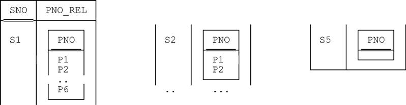
Relation Valued Attributes
To repeat, any type whatsoever—apart from the two exceptions noted in the section “Types” earlier—can be used as the basis for defining attributes of relations. In particular, relation types can be used for this purpose. (So too can tuple types.) Thus, attributes can be relation valued, meaning we can have relations with attributes whose values are relations in turn. An example of such a relation is shown, in outline, in Fig. 1.2.
Relations and Their Meaning
Note: The topic of this subsection is of crucial importance. We’ll be appealing to it repeatedly in the chapters to come, as you’ll quickly discover.
Given a relation r, the heading of r can be regarded as denoting a certain predicate, or in other words a truth valued function. Like all functions, that predicate has a set of parameters, and, because it’s truth valued, it returns a boolean value—TRUE or FALSE—when it’s invoked (i.e., when arguments are substituted for those parameters). The predicate corresponding to relation r is the relation predicate for r. Further, each tuple in the body of r can be regarded as denoting a certain proposition (where a proposition is a statement that’s unconditionally either true or false).11 The propositions in question represent invocations, or “instantiations,” of the relation predicate, obtained from that predicate by using values from the pertinent tuple as arguments to be substituted for the parameters. By way of example, consider the suppliers relation shown in Fig. 1.1. For that relation, the predicate, when expressed in the form of an English sentence, looks something like this:
Supplier SNO is under contract, is named SNAME, has status STATUS, and is located in city CITY
(the parameters here are SNO, SNAME, STATUS, and CITY, corresponding of course to the attributes of the relation). And the corresponding propositions, again when expressed as English sentences, are:
Supplier S1 is under contract, is named Smith, has status 20, and is located in city London
(obtained by substituting the SNO value S1, the NAME value Smith, the INTEGER value 20, and the CHAR value London for the appropriate parameters);
Supplier S2 is under contract, is named Jones, has status 10, and is located in city Paris
(obtained by substituting the SNO value S2, the NAME value Jones, the INTEGER value 10, and the CHAR value Paris for the appropriate parameters); and so on.
More generally, we can say the predicate corresponding to a given relation is the intended interpretation, or meaning, for that relation. And the propositions corresponding to tuples appearing in that relation are understood by convention to be ones that evaluate to TRUE. In other words, we subscribe, noncontroversially, to what’s called The Closed World Assumption. Here’s a definition:
Definition: Let relation r have predicate P. Then The Closed World Assumption (CWA) says: If tuple t appears in r, then the instantiation p of P corresponding to t is assumed to be true; conversely, if tuple t has the same heading as r but doesn’t appear in r, then the instantiation p of P corresponding to t is assumed to be false. In other words, a tuple appears in relation r if and only if it satisfies the predicate for r.
To say it another way: If relation r has predicate P, then the body of r contains all and only those tuples that correspond to instantiations of P that evaluate to TRUE.
By the way, it’s important to understand that every relation has an associated predicate, including in particular relations that are defined in terms of others by means of relational operators such as projection and join (see Chapter 2). For example, suppose we project the suppliers relation shown in Fig. 1.1 over the SNO, SNAME, and STATUS attributes (thereby effectively removing the CITY attribute). Then the predicate for the relation that results looks something like this:
There exists some city CITY such that supplier SNO is under contract, is named SNAME, has status STATUS, and is located in city CITY.
Observe that (as required) this predicate does have three parameters, not four, corresponding to the three attributes of the relation—CITY is now no longer a parameter but a bound variable instead, thanks to the fact that it’s quantified by the phrase “there exists some city. ” Note: Another and perhaps clearer way of making the same point (i.e., that the predicate has three parameters, not four) is to observe that the predicate as stated is logically equivalent to this one:
Supplier SNO is under contract, is named SNAME, has status STATUS, and is located somewhere (i.e., in some unspecified city).
This version of the predicate very clearly has just three parameters.
Relation Types Revisited
Earlier in this section, we said that if a given relation has heading H, then that relation is of type—relation type, that is—RELATION H. For example, the type of the suppliers relation from our running example is:
RELATION { SNO SNO , SNAME NAME , STATUS INTEGER , CITY CHAR }Of course, no significance attaches to the order in which the attributes happen to be specified within those enclosing braces, because there’s no left to right ordering to the attributes of a relation.
Now, there’s quite a bit more to be said about relation types in general; first, however, we need to take a closer look at tuple types. Let t be a tuple within the suppliers relation. Then t is of the following tuple type:
TUPLE { SNO SNO , SNAME NAME , STATUS INTEGER , CITY CHAR }(where, again, no significance attaches to the order in which the attributes are specified within the enclosing braces).
Observe now that, in contrast to the user defined scalar types SNO, NAME, and PNO, the foregoing tuple type—let’s call it STT—is not defined by means of a TYPE statement as such. Rather, the fact that the specified attribute types (SNO, NAME, INTEGER, and CHAR, in the case at hand) all exist is sufficient to ensure that type STT exists as well, albeit implicitly. In fact, every tuple type TT exists implicitly, just so long as every attribute of that tuple type TT is of some type that’s known to the system. For definiteness, however, let’s concentrate here on tuple type STT specifically:
■ Since there’s no TYPE statement for that type, there’s no associated possible representation (“possrep”) either.
■ Since there’s no possrep for that type, there aren’t any associated THE_ operators either.
■ However, there is an associated selector operator (in fact, every type has at least one associated selector). The easiest way to explain what an invocation of such a selector looks like is to show a simple BNF grammar fragment:12
<tuple selector invocation>
::= TUPLE { <component commalist> }<component>
::= <attribute name> <expression>
Here’s an example for tuple type STT:
TUPLE { SNO SNO ( 'S1' ) , SNAME NAME ( 'Smith' ) , STATUS 20 , CITY 'London' }This example is actually a tuple literal (which is a special case, of course)—it’s a literal because all of its component attribute values are specified as literals in turn—and it denotes precisely the tuple for supplier S1 from the suppliers relation as shown in Fig. 1.1. Of course, the order in which the components are specified is irrelevant.
Aside: When we say here that, e.g., the expression SNO ('S1') is a literal, we’re making tacit assumptions to the effect that (a) type SNO has a possrep also called—very likely by default—SNO, and further that (b) the possrep in question has a single component, of type CHAR. Similar remarks apply to types NAME and PNO also. End of aside.
Here’s another example, in which by contrast the component attribute values are mostly not specified as literals:
TUPLE { SNO SX , SNAME NMX, STATUS STX + 5 , CITY 'London' }Here, presumably, SX is a variable of type SNO, NMX is a variable of type NAME, and STX is a variable of type INTEGER.
One last point regarding tuple type STT: The fact is, that type—like all tuple types, at least so far as we’re concerned—is actually a generated type. A generated type is a type that’s obtained by invoking some type generator (in the example, the type generator is, specifically, TUPLE). You can think of a type generator as a special kind of operator; it’s special because (a) it returns a type instead of a value, and (b) it’s invoked at compile time instead of run time. For example, most programming languages support a type generator called ARRAY, which lets users define a variety of specific array types. In such a language, for example, the expression
ARRAY [ 1..10 ] OF INTEGER
might constitute an invocation of that type generator that returns a type consisting of all one-dimensional arrays with integer elements and with lower bound 1 and upper bound 10. In the same kind of way, the expression
TUPLE { SNO SNO , SNAME NAME, STATUS INTEGER , CITY CHAR }constitutes an invocation of the TUPLE type generator, and it returns a type consisting of all tuples whose attributes have the specified names and types—in other words, tuple type STT.
Turning now to relation types, almost everything we’ve been saying regarding tuple types applies to relation types as well, mutatis mutandis. For example, the relation type
RELATION { SNO SNO , SNAME NAME, STATUS INTEGER , CITY CHAR }—let’s call it SRT—is also not defined by means of a TYPE statement as such. Instead, the fact that the specified attribute types all exist is sufficient to ensure that type SRT exists as well, albeit implicitly. In fact, every relation type RT exists implicitly, just so long as every attribute of that relation type RT is of some type that’s known to the system. For definiteness, however, let’s concentrate here on type SRT specifically:
■ Since there’s no TYPE statement for that type, there’s no associated possible representation (“possrep”) either.
■ Since there’s no possrep for that type, there aren’t any associated THE_ operators either.
■ However, an associated selector operator does exist, and again the easiest way to explain it is by way of a simple BNF grammar fragment:13
<relation selector invocation>
::= RELATION [ <heading> ] <body>
<heading>
::= { <attribute name commalist> }<body>
::= { <tuple expression commalist> }Here’s an example for relation type SRT:
RELATION
{ TUPLE { SNO SNO ( 'S1' ) , SNAME NAME ( 'Smith' ) , STATUS 20, CITY 'London' } , TUPLE { SNO SNO ( 'S2' ) , SNAME NAME ( 'Jones' ) , STATUS 10 , CITY 'Paris' } , TUPLE { SNO SNO ( 'S3' ) , SNAME NAME ( 'Blake' ) , STATUS 30 , CITY 'Paris' } , TUPLE { SNO SNO ( 'S4' ) , SNAME NAME ( 'Clark' ) , STATUS 20 , CITY 'London' } , TUPLE { SNO SNO ( 'S5' ) , SNAME NAME ( 'Adams' ) , STATUS 30 , CITY 'Athens' } } ;This example is actually a relation literal (because the tuples that make up the body are all specified by means of literals in turn), and it denotes precisely the suppliers relation as shown in Fig. 1.1. (Of course, the order in which the tuples are specified is irrelevant. However, those tuples must certainly all be of the same tuple type—type STT, in fact, in the case at hand.) No explicit heading has been specified in this example, because the pertinent heading can obviously be inferred from the body. In fact, an explicit heading need be specified in a relation selector invocation if and only if the associated body is empty.
Providing an example in which the tuples are specified not as literals but as more general expressions is left as an exercise.
Finally, relation type SRT (like all relation types, in fact) is actually a generated type. That is, the expression
RELATION { SNO SNO , SNAME NAME, STATUS INTEGER , CITY CHAR }constitutes an invocation of the RELATION type generator, and it returns a type consisting of all relations with the specified heading—in other words, relation type SRT.
Exercises
1.1 Explain in your own words the terms type, possible representation, and selector.
1.2 Explain the difference between scalar and nonscalar types.
1.4 Write a Tutorial D definition for a read-only operator called DOUBLE that takes an integer and doubles it.
1.5 Repeat Exercise 1.4 but make the operator an update operator instead (i.e., the effect of invoking the operator should be to double the value assigned to a specified variable).
1.6 Define the terms heading, attribute, body, tuple, cardinality, and degree. By the way, the following facts are worth bearing in mind:
a. Every subset of a heading is a heading.
b. Every subset of a body is a body.
c. Every subset of a tuple is a tuple.
Aside: The term subset and various related terms are often used somewhat imprecisely in informal writing, and we therefore offer some brief (but accurate) definitions here. Let A and B be sets. Then “A is a subset of B” (or “A is included in B”), written A ⊆ B, means every element of A is also an element of B. By contrast, “A is a proper subset of B” (or “A is properly included in B”), written A ⊂ B, means A is a subset of B but there exists at least one element of B that isn’t also an element of A. So every set is a subset of itself, but no set is a proper subset of itself.
All of the foregoing applies to supersets also, mutatis mutandis. Thus, “B is a superset of A” (or “B includes A”), written B ⊇ A, means the same as “A is a subset of B.” Similarly, “B is a proper superset of A” (or “B properly includes A”), written B ⊃ A, means the same as “A is a proper subset of B.” So every set is a superset of itself, but no set is a proper superset of itself. End of aside.
1.7 State as precisely as you can what it means for two tuples t and t' to be duplicates of each other.
1.8 What’s a relation valued attribute?
1.9 Explain the term relation predicate.
1.10 Explain The Closed World Assumption.
1.12 Give an example of (a) a tuple literal, (b) a relation literal.
Answers
Most of the exercises in this chapter are really just review questions, and answers can be found in the body of the chapter. Here we give answers to Exercises 1.4 and 1.5 only.