Preliminaries
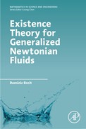
Abstract
In this chapter we present some preliminary material which will be needed in order to study non-stationary models for generalized Newtonian fluids. We begin with the functional analytic framework and define Bochner-spaces. After this we present the Lipschitz truncation method for non-stationary problems. Finally, we give a historical overview about the mathematical theory of weak solutions for non-stationary flows of power law fluids.
Keywords
Bochner spaces; Parabolic PDEs; Parabolic Lipschitz truncation; Whitney decomposition; Power law fluids; Historic comments on generalized Newtonian fluids
5.1 Bochner spaces
In the study of parabolic PDEs it is very useful to work with Banach space-valued mappings (see [143]). Let ![]() be a Banach space. A mapping
be a Banach space. A mapping ![]() is called a step function iff for some
is called a step function iff for some ![]()

where ![]() ,
, ![]() for
for ![]() and
and ![]() for
for ![]() . A function
. A function ![]() is called Bochner measurable iff there is a sequence
is called Bochner measurable iff there is a sequence ![]() of step functions such that
of step functions such that
for a.e. t. A function ![]() is called Bochner integrable iff there is a sequence
is called Bochner integrable iff there is a sequence ![]() of step functions such that (5.1.1) holds and
of step functions such that (5.1.1) holds and
The Bochner integral (as an element of ![]() ) is defined as
) is defined as

We define for ![]() and
and ![]() , the space
, the space ![]() to be the set of all Bochner measurable functions
to be the set of all Bochner measurable functions ![]() such that
such that

The space ![]() is the set of all Bochner measurable functions such that
is the set of all Bochner measurable functions such that
The space ![]() for
for ![]() is a Banach space together with the norm given above.
is a Banach space together with the norm given above.
Lemma 5.1.1
For ![]() we consider the distribution
we consider the distribution

Let ![]() be a Banach space with
be a Banach space with ![]() continuously. If there is
continuously. If there is ![]() such that
such that

we say that v is the weak derivative of u in ![]() and write
and write ![]() . The space
. The space ![]() consists of those functions from
consists of those functions from ![]() having weak derivatives in
having weak derivatives in ![]() . It is a Banach function space together with the norm
. It is a Banach function space together with the norm
Obviously this can be iterated to define the space ![]() .
.
In order to study the time regularity of functions from Bochner spaces we need to define different notations of continuity.
Definition 5.1.1
Let ![]() be a Banach space,
be a Banach space, ![]() and
and ![]() .
.
a) ![]() denotes the set of functions
denotes the set of functions ![]() being continuous with respect to the norm topology, i.e.
being continuous with respect to the norm topology, i.e.
for any sequence ![]() with
with ![]() .
.
b) ![]() denotes the set of functions
denotes the set of functions ![]() being continuous with respect to the weak topology, i.e.
being continuous with respect to the weak topology, i.e.
for any sequence ![]() with
with ![]() .
.
c) ![]() denotes the set of functions
denotes the set of functions ![]() being α-Hölder-continuous with respect to the norm topology, i.e.
being α-Hölder-continuous with respect to the norm topology, i.e.

Obviously, we have the inclusions
for any ![]() . The following variant of Sobolev's Theorem holds.
. The following variant of Sobolev's Theorem holds.
The following theorem shows how to obtain compactness in Bochner spaces. The original version is due to Aubin and Lions (see [14] and [109]) but does not include the case ![]() . The following more general version can be found in [128].
. The following more general version can be found in [128].
Theorem 5.1.22
In the context of stochastic PDEs we will be confronted with functions having only fractional derivatives in time. We define for ![]() and
and ![]() the norm
the norm

The space ![]() is now defined as the subspace of
is now defined as the subspace of ![]() consisting of the functions having finite
consisting of the functions having finite ![]() -norm. It can be shown that this is a complete space and we have
-norm. It can be shown that this is a complete space and we have ![]() . The following version of Theorem 5.1.22 holds (see [73]).
. The following version of Theorem 5.1.22 holds (see [73]).
Theorem 5.1.23
The following interpolation result is a special case of [8, Thm. 3.1]
Lemma 5.1.4

5.2 Basics on parabolic Lipschitz truncation
In this section we show how a Lipschitz truncation for non-stationary problems can be constructed. We follow the ideas of [65] (see [101] for a similar approach). Let ![]() be a space time cylinder. Let
be a space time cylinder. Let ![]() and
and ![]() satisfy
satisfy

Let ![]() . We say that
. We say that ![]() is an α-parabolic cylinder if
is an α-parabolic cylinder if ![]() . For
. For ![]() we define the scaled cylinder
we define the scaled cylinder ![]() . By
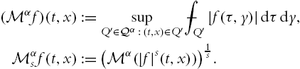
. By ![]() we denote the set of all α-parabolic cylinders. We define the α-parabolic maximal operators
we denote the set of all α-parabolic cylinders. We define the α-parabolic maximal operators ![]() and
and ![]() for
for ![]() by
by
It is standard [134] that for all ![]()
where the constants are independent of α. Another important tool is a parabolic Poincaré estimate for u in terms of ![]() and H, see Theorem B.1 of [65]: Let
and H, see Theorem B.1 of [65]: Let ![]() and any
and any ![]() with
with ![]() in
in ![]() for some
for some ![]() . Then the following holds
. Then the following holds

where c only depends on the dimension.
In order to define the Lipschitz truncation we have to cut large values of ![]() and H. We define the “bad set” as
and H. We define the “bad set” as
This is the set where we have to change u. In contrast to the stationary case discussed in Section 1.3, a straightforward argument is not available. So we follow the more flexible strategy based on a Whitney covering as done at the end of Section 3.1. According to Lemma 3.1 of [65] there exists an α-parabolic Whitney covering ![]() of
of ![]() .
.
Lemma 5.2.1
There is an α-parabolic Whitney covering ![]() of
of ![]() with the following properties.
with the following properties.
(PW1) ![]() ,
,
(PW2) for all ![]() we have
we have ![]() and
and ![]() ,
,
(PW3) if ![]() then
then ![]() ,
,
(PW4) at every point at most ![]() of the sets
of the sets ![]() intersect,
intersect,
where ![]() , the radius of
, the radius of ![]() and
and ![]() .
.
For each ![]() we define
we define ![]() . Note that
. Note that ![]() and
and ![]() for all
for all ![]() .
.
Lemma 5.2.2
There exists a partition of unity ![]() with respect to the covering
with respect to the covering ![]() from Lemma 5.2.1 such that
from Lemma 5.2.1 such that
(PP1) ![]() ,
,
(PP2) ![]() in
in ![]() ,
,
(PP3) ![]() .
.
Now we define
where ![]() . (In order to obtain a truncation with suitable properties up to the boundary one has to involve cut-off function as can be seen in [65] and Chapter 6. We neglect this for brevity.) We show first that the sum in (5.2.8) converges absolutely in
. (In order to obtain a truncation with suitable properties up to the boundary one has to involve cut-off function as can be seen in [65] and Chapter 6. We neglect this for brevity.) We show first that the sum in (5.2.8) converges absolutely in ![]() :
:

where we used (PP1) and the finite intersection property of ![]() (PW4). We proceed by showing the estimate for the gradient
(PW4). We proceed by showing the estimate for the gradient

where we used (PP3), (5.2.6) and (PW4). This shows that the definition in (5.2.8) makes sense. In particular we have

The truncation ![]() has better regularity properties than u; indeed,
has better regularity properties than u; indeed, ![]() is bounded by λ.
is bounded by λ.
Proof


The next lemma will control the time error we obtain when we use the truncation as a test function. We will only consider this from a formal point of view ignoring the technical difficulties connected with the distributional character of the time-derivative of u. We refer to [65, Thm. 3.9.(iii)] for a rigorous treatment.

Proof
We use Hölder's inequality, (PP3) and Lemma 6.1.10 to obtain

Note that we also took into account ![]() and that
and that ![]() is constant. Recalling the estimates in (5.2.10) and (5.2.6) we find that
is constant. Recalling the estimates in (5.2.10) and (5.2.6) we find that
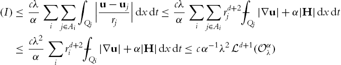
using (PW2), the definition of ![]() ,
, ![]() and the local finiteness of the
and the local finiteness of the ![]() . □
. □
Remark 5.2.9
As in Lemma 1.3.2 it is possible to have smallness of the level-sets in the sense that
with ![]() if
if ![]() . This and the choice
. This and the choice ![]() implies the smallness of the time error from Lemma 5.2.4. See [65, Section 4] for details.
implies the smallness of the time error from Lemma 5.2.4. See [65, Section 4] for details.
5.3 Existence results for power law fluids
The flow of a homogeneous incompressible fluid in a bounded body ![]() (
(![]() ) during the time interval
) during the time interval ![]() is described by the following set of equations
is described by the following set of equations

See for instance [23]. Here the unknown quantities are the velocity field ![]() and the pressure
and the pressure ![]() . The function
. The function ![]() represents a system of volume forces and
represents a system of volume forces and ![]() the initial datum, while
the initial datum, while ![]() is the stress deviator and
is the stress deviator and ![]() is the density of the fluid. Equation (5.3.11)1 and (5.3.11)2 describe the conservation of balance and the conservation of mass respectively. Both are valid for all homogeneous incompressible liquids and gases. In order to describe a specific fluid one needs a constitutive law relating the viscous stress tensor S to the symmetric gradient
is the density of the fluid. Equation (5.3.11)1 and (5.3.11)2 describe the conservation of balance and the conservation of mass respectively. Both are valid for all homogeneous incompressible liquids and gases. In order to describe a specific fluid one needs a constitutive law relating the viscous stress tensor S to the symmetric gradient ![]() of the velocity. In the simplest case this relation is linear, i.e.,
of the velocity. In the simplest case this relation is linear, i.e.,
where ![]() is the viscosity of the fluid. In this case we have
is the viscosity of the fluid. In this case we have ![]() and (5.3.11) is the famous Navier–Stokes equation. Its mathematical treatment started with the work of Leray and Ladyshenskaya (see [106]). The existence of a weak solution (where derivatives are to be understood in a distributional sense) can be established by nowadays standard arguments. However the regularity issue (i.e. the existence of a strong solution) is still open.
and (5.3.11) is the famous Navier–Stokes equation. Its mathematical treatment started with the work of Leray and Ladyshenskaya (see [106]). The existence of a weak solution (where derivatives are to be understood in a distributional sense) can be established by nowadays standard arguments. However the regularity issue (i.e. the existence of a strong solution) is still open.
As already motivated at the beginning of Chapter 4, a much more flexible model is
where ν is the generalized viscosity function. Of particular interest is the power law model
where ![]() and
and ![]() , cf. [13,23]. We recall that the case
, cf. [13,23]. We recall that the case ![]() covers many interesting applications.
covers many interesting applications.
In the following we give a historical overview concerning the theory of weak solutions to (5.3.11) and sketch the proofs, cf. [29]. It can be understood as the non-stationary counterpart to Section 1.4.
Monotone operator theory (1969).
Due to the appearance of the convective term ![]() the equations for power law fluids (the constitutive law is given by (5.3.11)) highly depend on the value of p. The first results were achieved by Ladyshenskaya and Lions for
the equations for power law fluids (the constitutive law is given by (5.3.11)) highly depend on the value of p. The first results were achieved by Ladyshenskaya and Lions for ![]() (see [106] and [109]). They showed the existence of a weak solution in the space
(see [106] and [109]). They showed the existence of a weak solution in the space
The weak formulation reads as

for all ![]() with S given by (5.3.14). In the case
with S given by (5.3.14). In the case ![]() it follows from parabolic interpolation that
it follows from parabolic interpolation that ![]() . So the weak solution is also a test-function and the existence proof is based on monotone operator theory and compactness arguments.
. So the weak solution is also a test-function and the existence proof is based on monotone operator theory and compactness arguments.
Let us assume that
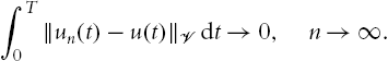
and that we have a sequence of approximated solutions, i.e.,
solving (5.3.15). A sequence of approximated solutions can be obtained, for instance via a Galerkin–Ansatz (see [111], Chapter 5). We want to pass to the limit. Assume further that
Then ![]() is also an admissible test-function (using (5.3.16)). We gain uniform a priori estimates and (after choosing an appropriate subsequence and applying Korn's inequality)
is also an admissible test-function (using (5.3.16)). We gain uniform a priori estimates and (after choosing an appropriate subsequence and applying Korn's inequality)

A parabolic interpolation implies
As in the stationary case, (5.3.14) yields together with (5.3.17)
A main difference to the stationary problem is the compactness of the velocity. Due to (5.3.17), (5.3.18) and (5.3.15) we can control the time derivative and have
Combining (5.3.17) and (5.3.20) the Aubin–Lions Compactness Theorem (cf. Theorem 5.1.22) yields
and together with (5.3.18)
Plugging the convergences (5.3.17)–(5.3.21) together we can pass to the limit in the approximate equation in all terms except for ![]() . As done in section 1.4 we have to apply arguments from monotone operator theory and show
. As done in section 1.4 we have to apply arguments from monotone operator theory and show

This follows along the same line as in the stationary case; the only term which needs a comment is the integral involving the time derivative. Here we have in addition to the terms from the stationary case the integral

using ![]() a.e., (5.3.17) and (5.3.20). As the integrand in (5.3.22) is non-negative the claim follows.
a.e., (5.3.17) and (5.3.20). As the integrand in (5.3.22) is non-negative the claim follows.
![]() -truncation (2007).
-truncation (2007).
The classical results have been improved by Wolf to the case ![]() via
via ![]() -truncation. In this situation we have
-truncation. In this situation we have ![]() and therefore we can test with functions from
and therefore we can test with functions from ![]() . The basic idea (which was already used in the stationary case in [78] together with the bound
. The basic idea (which was already used in the stationary case in [78] together with the bound ![]() ) is to approximate v by a bounded function
) is to approximate v by a bounded function ![]() which is equal to v on a large set and whose
which is equal to v on a large set and whose ![]() -norm can be controlled by L. Now we will present the approach developed in [140]. Note that the
-norm can be controlled by L. Now we will present the approach developed in [140]. Note that the ![]() -truncation has been used in the parabolic context before in [80] and [39]. Different from [140], both these papers deal with periodic and Navier's slip boundary conditions, respectively. So, the problems connected with the harmonic pressure do not occur.
-truncation has been used in the parabolic context before in [80] and [39]. Different from [140], both these papers deal with periodic and Navier's slip boundary conditions, respectively. So, the problems connected with the harmonic pressure do not occur.
Let us assume that
and the existence of approximate solutions ![]() to (5.3.15) with uniform a priori estimates in
to (5.3.15) with uniform a priori estimates in
Note that test-functions have to be bounded as we only have ![]() due to (5.3.23) and a parabolic interpolation. We have again the convergences (5.3.17)–(5.3.21) so we only have to establish the limit in
due to (5.3.23) and a parabolic interpolation. We have again the convergences (5.3.17)–(5.3.21) so we only have to establish the limit in ![]() . As the solution is not a test-function anymore we have to use some truncation. The
. As the solution is not a test-function anymore we have to use some truncation. The ![]() -truncation destroys the solenoidal character of a function and a correction via the Bogovskiĭ operator does not give the right sign when testing the time-derivative. So one has to introduce the pressure. In [140] this is done locally for the difference of approximate equation and limit equation. Due to the localization one has to use cut-off functions which we neglect in the following as they only produce additional terms of lower order. We have
-truncation destroys the solenoidal character of a function and a correction via the Bogovskiĭ operator does not give the right sign when testing the time-derivative. So one has to introduce the pressure. In [140] this is done locally for the difference of approximate equation and limit equation. Due to the localization one has to use cut-off functions which we neglect in the following as they only produce additional terms of lower order. We have

for all ![]() with
with

where ![]() , cf. (5.3.23). Now we can introduce a pressure
, cf. (5.3.23). Now we can introduce a pressure ![]() and decompose it into
and decompose it into ![]() such that
such that

for all ![]() . The pressure
. The pressure ![]() is harmonic whereas
is harmonic whereas ![]() and
and ![]() feature the same convergences properties as
feature the same convergences properties as ![]() and
and ![]() respectively (see (5.3.25)). Now we test (5.3.15) with the
respectively (see (5.3.25)). Now we test (5.3.15) with the ![]() -truncation of
-truncation of ![]() . The result is the same as in the stationary case (cf. Section 1.4) since the term involving the time-derivative has the right sign. Finally we have
. The result is the same as in the stationary case (cf. Section 1.4) since the term involving the time-derivative has the right sign. Finally we have

and due to (5.3.17) and ![]()

We can finish the proof as in the stationary case; the additional function ![]() is compact (harmonic in space and bounded in time).
is compact (harmonic in space and bounded in time).
Lipschitz truncation (2010).
Wolf's result was improved to
in [65] by the Lipschitz truncation method. Under this restriction to p we have ![]() which means we can test by functions having bounded gradients. So one has to approximate v by a Lipschitz continuous function
which means we can test by functions having bounded gradients. So one has to approximate v by a Lipschitz continuous function ![]() . The best result so far has been shown in [65] by a parabolic Lipschitz truncation, see Section 5.2 for more details. Let us assume that (5.3.27) holds and that there is a sequence of approximate solutions
. The best result so far has been shown in [65] by a parabolic Lipschitz truncation, see Section 5.2 for more details. Let us assume that (5.3.27) holds and that there is a sequence of approximate solutions ![]() to (5.3.15) with uniform estimates in
to (5.3.15) with uniform estimates in ![]() . On account of (5.3.27) we have
. On account of (5.3.27) we have ![]() such that test-functions must have bounded gradients. We have again the convergences (5.3.17)–(5.3.21) so we only have to establish the limit in
such that test-functions must have bounded gradients. We have again the convergences (5.3.17)–(5.3.21) so we only have to establish the limit in ![]() .
.
In contrast to the stationary Lipschitz truncation explained in Section 1.4, the parabolic version requires a suitable scaling of the Whitney cubes ![]() . To be precise, they shall be of the form
. To be precise, they shall be of the form
with ![]() (λ is the Lipschitz constant of the truncation). The reason for this is the control of the distributional time derivative. Despite the
(λ is the Lipschitz constant of the truncation). The reason for this is the control of the distributional time derivative. Despite the ![]() -truncation the Lipschitz truncation is not only nonlinear but also nonlocal. So the term involving the time derivative does not have a sign. But due to (5.3.28) it is possible to show that
-truncation the Lipschitz truncation is not only nonlinear but also nonlocal. So the term involving the time derivative does not have a sign. But due to (5.3.28) it is possible to show that

recalling Lemma 5.2.4. On account of this the Lipschitz truncation can be roughly speaking applied as in the stationary case in Section 1.4. However, there are certain technical difficulties. First of all, the known parabolic versions of the Lipschitz truncation work only locally. So, one has to involve bubble functions in order to localize the arguments. The approach in [65] introduces the pressure function as explained in (5.3.26) for the parabolic ![]() -truncation. In fact, the authors use the Lipschitz truncation of the function
-truncation. In fact, the authors use the Lipschitz truncation of the function ![]() .
.