
The A -Stokes system
The aim of this section is to present regularity results for the (non-stationary) A![]() -Stokes system depending on the right hand side (in divergence form). Let us fix for this section a bounded domain G⊂R3
-Stokes system depending on the right hand side (in divergence form). Let us fix for this section a bounded domain G⊂R3![]() with C2
with C2![]() -boundary and a time interval (0,T)
-boundary and a time interval (0,T)![]() . Moreover, let A:R3×3→R3×3
. Moreover, let A:R3×3→R3×3![]() be an elliptic tensor.
be an elliptic tensor.
B.1 The stationary problem
The A![]() -Stokes problem (in the pressure-free formulation) with right hand side f∈L1(G)
-Stokes problem (in the pressure-free formulation) with right hand side f∈L1(G)![]() reads as: find v∈LD0,div(G)
reads as: find v∈LD0,div(G)![]() such that
such that
∫GA(ε(v),ε(φ))dx=∫Gf⋅φdxfor allφ∈C∞0,div(G).

The right hand side can also be given in divergence form, i.e.
∫GA(ε(v),ε(φ))dx=∫GF:∇φdxfor allφ∈C∞0,div(G)

for F∈L1(G)![]() . For certain purposes it is convenient to discuss the problem with a fixed divergence. To be precise for g∈L1⊥(G)
. For certain purposes it is convenient to discuss the problem with a fixed divergence. To be precise for g∈L1⊥(G)![]() we are seeking for a function v∈LD0(G)
we are seeking for a function v∈LD0(G)![]() with divv=g
with divv=g![]() satisfying (B.1.1) or (B.1.2). We have the following Lq
satisfying (B.1.1) or (B.1.2). We have the following Lq![]() -estimates.
-estimates.
Lemma B.1.1
Let G⊂R3![]() be a bounded C2
be a bounded C2![]() -domain and 1<q<∞
-domain and 1<q<∞![]() .
.
a) Let f∈Lq(G)![]() and g∈W1,q(G)
and g∈W1,q(G)![]() with ∫Ggdx=0
with ∫Ggdx=0![]() . Then there is a unique solution w∈W2,q∩W1,q0(G)
. Then there is a unique solution w∈W2,q∩W1,q0(G)![]() to (B.1.1) such that divv=g
to (B.1.1) such that divv=g![]() and
and
⨍B|∇2w|qdx⩽c⨍G|f|qdx+c⨍G|∇g|qdx,

where c only depends on A![]() and q.
and q.
b) Let F∈Lq(G)![]() and g∈Lq0(G)
and g∈Lq0(G)![]() . Then there is a unique solution w∈W1,q0(G)
. Then there is a unique solution w∈W1,q0(G)![]() to (B.1.2) such that divv=g
to (B.1.2) such that divv=g![]() and
and
⨍G|∇w|qdx⩽c⨍G|F|qdx+c⨍G|g|qdx,

where c only depends on A![]() and q.
and q.
In case A=I![]() both parts follow from [10], Thm. 4.1. However, the main tool in [10] is the theory from [6,7] where very general linear systems are investigated. Hence it is clear that the results also hold in case of an arbitrary elliptic tensor A
both parts follow from [10], Thm. 4.1. However, the main tool in [10] is the theory from [6,7] where very general linear systems are investigated. Hence it is clear that the results also hold in case of an arbitrary elliptic tensor A![]() .
.
Corollary B.1.1
Let the assumptions of Lemma B.1.1 be satisfied. Assume further that f=0![]() and
and
g=divg+g0
with g∈W1,q(G)![]() and g0∈Lq0(G)
and g0∈Lq0(G)![]() with sptg0⋐G
with sptg0⋐G![]() . Then we have
. Then we have
∫G|w|qdx⩽c∫G|g|qdx+c∫∂G|g⋅N|qdH2+cL3(sptg0)β∫G|g0|qdx

for some β>0![]() .
.
Proof
We follow the lines of [133, Thm. 2.4]. Let ψ∈Lq′(G)![]() be arbitrary. In accordance to Lemma B.1.1 a) there is a unique solution u∈W2,q′∩W1,q′0,div(G)
be arbitrary. In accordance to Lemma B.1.1 a) there is a unique solution u∈W2,q′∩W1,q′0,div(G)![]() to the A
to the A![]() -Stokes problem with right-hand-side ψ such that
-Stokes problem with right-hand-side ψ such that
∫G|∇2u|q′dx⩽c∫G|ψ|q′dx.

By De Rahm's theorem there is a unique ϑ∈Lq′⊥(G)![]() such that
such that
∫GA(ε(u),ε(φ))dx=∫Gϑdivφ+∫Gψ⋅φdxfor all φ∈W1,q0(G).

We can conclude that ϑ∈W1,q′(G)![]() with
with
⨍G|∇ϑ|q′dx⩽c(⨍G|∇2u|q′dx+⨍G|ψ|q′dx)⩽c⨍G|ψ|q′dx.

We proceed by
∫Gw⋅ψdx=∫GA(ε(u),ε(w))dx−∫Gϑdivwdx=−∫Gϑdivwdx=−∫Gϑdivgdx−∫Gg0ϑdx=∫G∇ϑ⋅gdx−∫∂Gg⋅NϑdH2−∫Gg0ϑdx.

We finish the proof by estimating this integrals separately using (B.1.4). For the first one we obtain
|∫G∇ϑ⋅gdx|⩽(∫G|∇ϑ|q′dx)1q′(∫G|g|qdx)1q⩽(∫G|ψ|q′dx)1q′(∫G|g|qdx)1q.

Similarly, we estimate using the trace theorem
|∫∂Gϑg⋅NdH2|⩽(∫∂G|ϑ|q′dH2)1q′(∫∂G|g⋅N|qdH2)1q⩽(∫G|∇ϑ|q′dx)1q′(∫∂G|g⋅N|qdH2)1q⩽(∫G|ψ|q′dx)1q′(∫∂G|g⋅N|qdH2)1q.

In case q′<3![]() we obtain for the third integral
we obtain for the third integral
|∫Gg0ϑdx|⩽(∫G|ϑ|3q′3−q′dx)3−q′dq′(∫G|g0|3q′4q′−3dx)4q′−33q′⩽(∫G|∇ϑ|q′dx)q′L3(sptg0)β(∫G|g0|qdx)1q⩽(∫G|ψ|q′dx)1q′L3(sptg0)β(∫G|g0|qdx)1q,

where β=13![]() . If q′⩾3
. If q′⩾3![]() we can modify the proof by replacing 3q′3−q′
we can modify the proof by replacing 3q′3−q′![]() with an arbitrary number r>q′
with an arbitrary number r>q′![]() and choose β=3r′
and choose β=3r′![]() . As ψ is arbitrary, the claim follows. □
. As ψ is arbitrary, the claim follows. □
B.2 The non-stationary problem
Now we turn to the parabolic problem and the first result is a local Lq![]() -estimate for weak solutions. In case of the A
-estimate for weak solutions. In case of the A![]() -heat system this follows from the continuity of the corresponding semigroup (see [132]). It is also known for the non-stationary Stokes-system (see [133] and [88]) but not in our setting.
-heat system this follows from the continuity of the corresponding semigroup (see [132]). It is also known for the non-stationary Stokes-system (see [133] and [88]) but not in our setting.
Theorem B.2.48


Proof
The main ingredient is the proof of the following auxiliary result which has been used in a similar version in [42].
i) We start with interior estimates. Let
Qr:=Qr(x0,t0):=(t0−r2,t0+r2)×Br(x0)
be a parabolic cylinder such that 4Qr⊂Q0![]() . We claim the following: There is a constant N1>0
. We claim the following: There is a constant N1>0![]() such that for every ε>0
such that for every ε>0![]() there is δ=δ(ε)>0
there is δ=δ(ε)>0![]() such that (since f∈L2(0,T;L2loc(R3))
such that (since f∈L2(0,T;L2loc(R3))![]() the standard interior regularity theory implies ∇2v∈L2(0,T;L2loc(R3))
the standard interior regularity theory implies ∇2v∈L2(0,T;L2loc(R3))![]() and ∂tv∈L2(0,T;L2loc(R3))
and ∂tv∈L2(0,T;L2loc(R3))![]() )
)
L4(Qr∩{M(|f|)2>N21})⩾εL4(Qr)⇒Qr⊂{M(|∇2v|2)>1}∪{M(|f|2)>δ2}.

Let us assume for simplicity that r=1![]() . In fact, we will establish (B.2.6) by showing
. In fact, we will establish (B.2.6) by showing
Q1∩{M(|∇2v|2)⩽1}∩{M(|f|2)⩽δ2}≠∅⇒L4(Q1∩{M(|∇v|)2>N21})<εL4(Q1)

and applying a simple scaling argument. In order to show (B.2.7) we compare v with a solution to a homogeneous problem on
Q4=(t40−42,t40+42)×B4(x40)⊂Q0
which is smooth in the interior. So let us define h as the unique solution to
{∂th−divA(ε(h))=∇πhin Q4,divh=0in Q4,h=von I4×∂B4,h(t40,⋅)=v(t40,⋅)in B4.

We test the difference of both equations with v−h![]() . This yields by the ellipticity of A
. This yields by the ellipticity of A![]()
supt∈I4∫B4|v(t)−h(t)|2dx+∫Q4|ε(v)−ε(h)|2dxdt⩽c∫Q4|f|2dxdt+c∫Q4|v−h|2dxdt.

An application of Korn's inequality and Gronwall's lemma implies
supt∈I4∫B4|v(t)−h(t)|2dx+∫Q4|∇v−∇h|2dxdt⩽c∫Q4|f|2dxdt.

First we insert ∂t(v−h)![]() which yields similarly
which yields similarly
∫Q4|∂t(v−h)|2dx+supt∈I4∫B4|∇v−∇h|2dx⩽c∫Q4|f|2dxdt.

We can introduce the pressure terms πv,πh∈L2(I4,L20(B4))![]() in the equations for v and h and show
in the equations for v and h and show
∫Q4|πv−πh|2dx⩽c∫Q4|f|2dxdt.

Estimate (B.2.11) can be shown by using the Bogovskiĭ operator, see Section 2.1. Setting Bog=BogB4![]() we gain due to (B.2.10) for any φ∈C∞0(Q4)
we gain due to (B.2.10) for any φ∈C∞0(Q4)![]() that
that
∫Q4(πv−πh)φdxdt=∫Q4(πv−πh)divBog(φ−φB4)dxdt=∫Q4A(ε(v−h),ε(Bog(φ−φB4)))dxdt+∫Q4f⋅Bog(φ−φB4))dxdt−∫Q4∂t(v−h)⋅Bog(φ−φB4)dxdt⩽c(‖∇(v−h)‖2+‖f‖2+‖∂t(v−h)‖2)‖∇Bog(φ−(φ)B4)‖2⩽c(∫Q4|f|2dxdt)12(∫Q4|φ|2dxdt)12.

Now we choose a cut off function η∈C∞0(B4)![]() with 0⩽η⩽1
with 0⩽η⩽1![]() and η≡1
and η≡1![]() on B3
on B3![]() . We insert ∂γ(η2∂γ(v−h))
. We insert ∂γ(η2∂γ(v−h))![]() in the equation for v−h
in the equation for v−h![]() and sum over γ∈{1,2,3}
and sum over γ∈{1,2,3}![]() . We gain
. We gain
supt∈I4∫B4η2|∇(v−h)|2dx+∫Q4η2|∇ε(v)−∇ε(h)|2dxdt⩽c∫Q4f⋅∂γ(η2∂γ(h−h))dxdt+c(∇η)∫Q4|∇v−∇h|2dxdt+c∫Q4(π−πh)⋅∂γ(∇η2⋅∂γ(h−h))dxdt.

We estimate the term involving f by
∫Q4f⋅∂γ(η2∂γ(v−h))dxdt⩽c(κ)∫Q4|f|2dxdt+κ∫Q4η2|∇2v−∇2h|2dxdt+c(∇η)∫Q4|∇v−∇h|2dxdt,

where κ>0![]() is arbitrary. The term involving π−πh
is arbitrary. The term involving π−πh![]() can be estimated in the same fashion. Choosing κ>0
can be estimated in the same fashion. Choosing κ>0![]() small enough and using the inequality |∇2u|⩽c|∇ε(u)|
small enough and using the inequality |∇2u|⩽c|∇ε(u)|![]() as well as (B.2.9)–(B.2.11) shows
as well as (B.2.9)–(B.2.11) shows
supt∈I4∫B3|∇(v−h)(t)|2dx+∫I4∫B3|∇2v−∇2h|2dxdt⩽c∫Q4|f|2dxdt.

Now, let us assume that (B.2.7)1 holds. Then there is a point (t0,x0)∈Q1![]() such that
such that
⨍Qσ(t0,x0)|∇2v|2dxdt⩽1,⨍Qσ(t0,x0)|f|2dxdt⩽δ2
for all σ>0![]() . Since Q4⊂Q6(t0,x0)
. Since Q4⊂Q6(t0,x0)![]() we have
we have
∫Q4|∇2v|2dxdt⩽c,∫Q4|f|2dxdt⩽cδ2.

As h is smooth we know that
N20:=supQ3|∇2h|2<∞.
From this we aim to conclude that
Q1∩{M(|∇2v|2)>N21}⊂Q1∩{M(χQ3|∇2v−∇2h|2)>N20}
for N21:=max{4N20,25}![]() . To establish (B.2.16) suppose that
. To establish (B.2.16) suppose that
(t,x)∈Q1∩{M(χQ3|∇2v−∇2h|2)⩽N20}.
If σ⩽2![]() we have Qσ(t,x)⊂Q3
we have Qσ(t,x)⊂Q3![]() and gain by (B.2.15)
and gain by (B.2.15)
⨍Qσ(t,x)|∇2v|2dxdt⩽2⨍Qσ(t,x)χQ3|∇2v−∇2h|2dxdt+2⨍Qσ(t,x)χQ3|∇2h|2dxdt⩽4N20.

If σ⩾2![]() we have by (B.2.13)
we have by (B.2.13)
⨍Qσ(t,x)|∇2v|2dxdt⩽25⨍Q2σ(t0,x0)|∇2v|2dxdt⩽25.

Combining the both cases yields (B.2.16). This implies together with the continuity of the maximal function on L2![]() , (B.2.12) and (B.2.14)
, (B.2.12) and (B.2.14)
L4(Q1∩{M(|∇2v|2)>N21})⩽Ld+1(Q1∩{M(χQ3|∇2v−∇2h|2)>N20})⩽cN20∫Q3|∇2v−∇2h|2dxdt⩽cN20∫Q3|f|2dxdt⩽cN20δ2=εL4(Q1),

choosing δ:=c−1/2N0√ε![]() . So we have shown (B.2.7) which yields (B.2.6) by a scaling argument.
. So we have shown (B.2.7) which yields (B.2.6) by a scaling argument.
If (B.2.6)1 holds then we have
L4(Qr∩{M(|∇2v|)2>N21})⩽εL4(Qr∩{M(|∇2v|2)>1}∪{M(|f|2)>δ2})⩽ε(L4(Qr∩{M(|∇2v|2)>1})+L4(Qr∩{M(|f|2)>δ2})).

Multiplying the equation for v by some small number ϱ=ϱ(‖f‖q,‖∇2v‖2)![]() we can assume that
we can assume that
L4(Qr∩{M(|∇2v|2)>N21})<ε.
By induction we can establish that
L4(Qr∩{M(|∇2v|2)>N2k1})⩽εkL4(Qr∩{M(|∇2v|2)>1}+ck∑i=1εiL4(Qr∩{M(|f|2)>δ2N2(k−i)1}).

In the induction step one has to introduce v1:=vN1![]() which is a solution to the A
which is a solution to the A![]() -Stokes problem with right hand side f1:=fN1
-Stokes problem with right hand side f1:=fN1![]() . Now we will show ∇2v∈Lq(Qr)
. Now we will show ∇2v∈Lq(Qr)![]() . For this we use the equivalence for 1⩽q0<∞
. For this we use the equivalence for 1⩽q0<∞![]()
∞∑k=1Lq0kL4(Qr∩{(t,x):|u(t,x)|>θLk})<∞⇔u∈Lq0(Qr),

which holds for any measurable function u, see [44]. Here L>1![]() and θ>0
and θ>0![]() are arbitrary. So we aim to prove that
are arbitrary. So we aim to prove that
∞∑k=1(N21)q2kL4(Qr∩{M(|∇2v|2)>N2k1})<∞

to conclude M(|∇2v|2)∈Lq2(Qr)![]() and hence ∇2v∈Lq(Qr)
and hence ∇2v∈Lq(Qr)![]() . Since f∈Lq(Qr)
. Since f∈Lq(Qr)![]() we have M(|f|2)∈Lq/2(Qr)
we have M(|f|2)∈Lq/2(Qr)![]() (recall (5.2.4)) and we have
(recall (5.2.4)) and we have
∞∑k=1(N21)q2kL4(Qr∩{M(|f|2)>δ2N2k1})<∞.

We obtain
∞∑k=1(N1)qkL4(Qr∩{M(|∇2v|2)>N2k1})⩽c∞∑k=1(N1)qkεkL4(Qr∩{M(|∇2v|2)>1})+c∞∑k=1(N1)qkk∑i=1εiL4(Qr∩{M(|f|2)>δ2N2(k−i)1})⩽cr∞∑k=1(εN1)qk+c∞∑i=1εi(N1)qi∞∑k=i(N1)q(k−i)L4(Qr∩{M(|f|2)>δ2N2(k−i)1})⩽cr∞∑k=1(εNq1)k.

If we choose εNq1<1![]() the sum in (B.2.19) is converging and we have ∇2v∈Lq(Qr)
the sum in (B.2.19) is converging and we have ∇2v∈Lq(Qr)![]() . Since the mapping f↦∇2v
. Since the mapping f↦∇2v![]() is linear we gain the desired estimate
is linear we gain the desired estimate
∫Qr|∇2v|qdxdt⩽cr∫Q0|f|qdxdt.

ii) Now let Q1![]() be a cylinder such that 4Q1∩(−∞,0]×R3≠∅
be a cylinder such that 4Q1∩(−∞,0]×R3≠∅![]() . Moreover, assume that Q1∩Q0≠∅
. Moreover, assume that Q1∩Q0≠∅![]() . We consider the solution ˜h
. We consider the solution ˜h![]() to
to
{∂t˜h−divA(ε(˜h))=∇π˜hin ˜Q4,div˜h=0in ˜Q4,˜h=von ˜I4×∂B4,˜h(t40,⋅)=0in B4,

where ˜Im:=Im∩(0,T)![]() and ˜Qm:=˜Im×Bm
and ˜Qm:=˜Im×Bm![]() . We can establish a variant of (B.2.12) on ˜Q4
. We can establish a variant of (B.2.12) on ˜Q4![]() . Now we have sup˜Q3|∇2˜h|2<∞
. Now we have sup˜Q3|∇2˜h|2<∞![]() due to the smooth initial datum of ˜h
due to the smooth initial datum of ˜h![]() (recall that v(0,⋅)=0
(recall that v(0,⋅)=0![]() a.e.). So we can finish the proof as before and gain ∇2v∈Lq(Q1)
a.e.). So we can finish the proof as before and gain ∇2v∈Lq(Q1)![]() . This implies again (B.2.20).
. This implies again (B.2.20).
iii) The situation 4Q1∩[T,∞)×R3≠∅![]() is uncritical again and we can assume that ii) and iii) do not occur for the same cylinder (by choosing sufficiently small cubes).
is uncritical again and we can assume that ii) and iii) do not occur for the same cylinder (by choosing sufficiently small cubes).
Covering the set (0,T)×B![]() by smaller cylinders and combing i)–iii) yield the desired estimate. □
by smaller cylinders and combing i)–iii) yield the desired estimate. □
Corollary B.2.1
Under the assumptions of Theorem B.2.48 we have for all balls B⊂R3![]() the following estimates for some constant cB
the following estimates for some constant cB![]() which does not depend on T.
which does not depend on T.
a) The following holds
T∫0∫B(|vT|q+|∇v√T|q+|∇2v|q)dxdt⩽cB∫Q0|f|qdxdt.

b) We have ∂tv∈Lq(0,T;Lqloc(R3))![]() together with
together with
T∫0∫B|∂tv|qdxdt⩽cB∫Q0|f|qdxdt.

c) There is π∈Lq((0,T),W1,qloc(R3))![]() such that
such that
∫Q0v⋅∂tφdxdt−∫Q0A(ε(v),ε(φ))dx=∫Q0πdivφdxdt+∫Q0f⋅φdxdt

for all φ∈C∞0([0,T)×R3)![]() .
.
d) The following holds
T∫0∫B(|π√T|q+|∇π|q)dxdt⩽cB∫Q0|f|qdxdt.

Proof
The estimate in a) is a simple scaling argument. Having a solution v defined on (0,T)×R3![]() we gain a solution ˆv
we gain a solution ˆv![]() on (0,1)×R3
on (0,1)×R3![]() by setting
by setting
ˆv(s,x):=1Tv(Ts,√Tx).
Now we apply Theorem B.2.48 to ˆv![]() . The constant which appears is independent of T. Transforming back to v yields the claimed inequality.
. The constant which appears is independent of T. Transforming back to v yields the claimed inequality.
b) For φ∈C∞0(Q0)![]() with φ(t,x)=τ(t)ψ(x)
with φ(t,x)=τ(t)ψ(x)![]() where φ∈C∞0(G)
where φ∈C∞0(G)![]() (G∈R3
(G∈R3![]() a bounded Lipschitz domain) we have
a bounded Lipschitz domain) we have
∫Q0v⋅∂tφdxdt=T∫0∂tτ∫R3v⋅(ψdiv+∇Ψ)dxdt=T∫0∂tτ∫R3v⋅ψdivdxdt=∫Q0v⋅∂tφdivdxdt

where ψdiv:=ψ−∇Δ−1Gdivψ![]() and Ψ:=Δ−1Gdivψ
and Ψ:=Δ−1Gdivψ![]() . (Here Δ−1G
. (Here Δ−1G![]() is the solution operator to the Laplace equation with zero boundary datum on ∂G.) Here we took into account Ψ|∂G=0
is the solution operator to the Laplace equation with zero boundary datum on ∂G.) Here we took into account Ψ|∂G=0![]() as well as divv=0
as well as divv=0![]() . Using ∇2v∈L2(0,T;L2loc(R3))
. Using ∇2v∈L2(0,T;L2loc(R3))![]() we proceed by
we proceed by
∫Q0v⋅∂tφdxdt=T∫0∫G(f−divAε(v))⋅φdivdxdt⩽c(T∫0∫G(|∇2v|q+|f|q)dxdt)1q(T∫0∫G|φdiv|q′dxdt)1q′⩽c(∫Q0|f|qdxdt)1q(T∫0∫G|φ|q′dxdt)1q′.
In the last step we used the estimate from Theorem B.2.48 and continuity of ∇Δ−1Gdiv![]() on Lq′(G)
on Lq′(G)![]() . Duality implies ∂tv∈Lq(0,T;Lqloc(R3))
. Duality implies ∂tv∈Lq(0,T;Lqloc(R3))![]() and we can introduce the pressure function π∈Lq(0,T;Lqloc(R3))
and we can introduce the pressure function π∈Lq(0,T;Lqloc(R3))![]() as claimed in b) by De Rahm's Theorem. Using the equation for v and the estimates in a) and b) we gain
as claimed in b) by De Rahm's Theorem. Using the equation for v and the estimates in a) and b) we gain
∫Q|∇π|qdxdt⩽c∫Q0|f|qdxdt.

The estimate for π in d) follows again by scaling. □
Corollary B.2.2
Let f∈Lq(Q+0)![]() for some q>2
for some q>2![]() where Q+0:=(0,T)×R3+
where Q+0:=(0,T)×R3+![]() , R3+=R3∩[x3>0]
, R3+=R3∩[x3>0]![]() , and let v∈L2((0,T);W1,20,div(R3+))
, and let v∈L2((0,T);W1,20,div(R3+))![]() with v|x3=0=0
with v|x3=0=0![]() be the unique weak solution to
be the unique weak solution to
∫Q+0v⋅∂tφdxdt−∫Q+0A(ε(v),ε(φ))dx=∫Q+0f⋅φdxdt

for all φ∈C∞0,div([0,T)×R3+)![]() . Then the results from Theorem B.2.48 and Corollary B.2.1 hold for v for all half balls B+(z)=B(z)∩[x3>0]⊂R3
. Then the results from Theorem B.2.48 and Corollary B.2.1 hold for v for all half balls B+(z)=B(z)∩[x3>0]⊂R3![]() with z3=0
with z3=0![]() .
.
Proof
We will show a variant of the Lq![]() -estimate from Theorem B.2.48 on half balls B+
-estimate from Theorem B.2.48 on half balls B+![]() , i.e.
, i.e.
T∫0∫B+|∇2v|qdxdt⩽cBT∫0∫Q+|f|qdxdt.

From this we can follow estimates in the fashion of Corollary B.2.1 as done there. In order to establish (B.2.23) we will proceed as in the proof of Theorem B.2.48 replacing all balls with half ball. So let Q1⊂R4![]() such that 4Q1⊂Q0
such that 4Q1⊂Q0![]() (the other situation can be shown along the modifications indicated at the end of the proof of Theorem B.2.48). Moreover, assume that Q1=I1×B1(z)
(the other situation can be shown along the modifications indicated at the end of the proof of Theorem B.2.48). Moreover, assume that Q1=I1×B1(z)![]() where z3=0
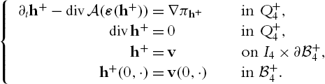
where z3=0![]() . We compare v with the unique solution h+
. We compare v with the unique solution h+![]() to
to
{∂th+−divA(ε(h+))=∇πh+in Q+4,divh+=0in Q+4,h+=von I4×∂B+4,h+(0,⋅)=v(0,⋅)in B+4.
We gain a version of the estimate (B.2.9) and (B.2.10) on half-balls. In fact, there holds
supt∈I4∫B+4|v−h+|2dx+∫Q+4|∇v−∇h+|2dxdt⩽c∫Q+4|f|2dxdt,

∫Q+4|∂t(v−h+)|2dx+supt∈I4∫B+4|∇v−∇h+|2dx⩽c∫Q+4|f|2dxdt.

We can introduce the pressure terms πv,πh+∈L2(I4,L20(B+4))![]() in the equations for v and h+
in the equations for v and h+![]() and show
and show
∫Q+4|πv−πh+|2dx⩽c∫Q+4|f|2dxdt.

This can be done as in the proof of (B.2.11) using the Bogovskiĭ operator on B+4![]() . Estimate (B.2.27) can be shown by using the Bogovskiĭ operator introduced in [24]. Now we insert ∂γ(η2∂γ(v−h))
. Estimate (B.2.27) can be shown by using the Bogovskiĭ operator introduced in [24]. Now we insert ∂γ(η2∂γ(v−h))![]() for γ∈{1,2}
for γ∈{1,2}![]() in the equation for v−h
in the equation for v−h![]() . Here we choose η∈C∞0(B4)
. Here we choose η∈C∞0(B4)![]() with 0⩽η⩽1
with 0⩽η⩽1![]() and η≡1
and η≡1![]() on B3
on B3![]() . This yields together with (B.2.25)–(B.2.27)
. This yields together with (B.2.25)–(B.2.27)
∫Q+3|˜∇∇(v−h)|2dx⩽c∫Q+4|f|2dxdt,

where ˜∇:=(∂1,∂2)![]() . Finally, the only term which is missing is ∂23(v−h)
. Finally, the only term which is missing is ∂23(v−h)![]() . On account of div(v−h)=0
. On account of div(v−h)=0![]() we have (cf. [21])
we have (cf. [21])
|∂23(v−h)|⩽c(|˜∇(πv−πh+)|+|˜∇∇(v−h)|+|f|).
So we have to estimate derivatives of the pressure. In fact we have
∫Q+3|˜∇(πv−πh+)|2dx⩽c∫Q+4|f|2dxdt.

We can show this similarly to the proof of (B.2.27) replacing φ by ∂γφ![]() and using (B.2.28). Combining (B.2.28)–(B.2.30) implies
and using (B.2.28). Combining (B.2.28)–(B.2.30) implies
∫Q+3|∇2v−∇2h|2dx⩽c∫Q+4|f|2dxdt.

Moreover, we know supQ+3|∇2h+|2<∞![]() . Note that h+=0
. Note that h+=0![]() on Q3∩[x3=0]
on Q3∩[x3=0]![]() . This allows to show ∇2v∈Lq(Q+1)
. This allows to show ∇2v∈Lq(Q+1)![]() as in the proof of Theorem B.2.48. □
as in the proof of Theorem B.2.48. □
Corollary B.2.3
Let f∈Lq(Qν,ξ0)![]() for some q>2
for some q>2![]() where Qν,ξ0:=(0,T)×R3ν,ξ
where Qν,ξ0:=(0,T)×R3ν,ξ![]() , R3ν,ξ=R3∩[(x−ξ)⋅ν>0]
, R3ν,ξ=R3∩[(x−ξ)⋅ν>0]![]() for some ν,ξ∈R3
for some ν,ξ∈R3![]() . Let v∈L2(0,T;W1,20,div(R3ν,ξ))
. Let v∈L2(0,T;W1,20,div(R3ν,ξ))![]() with v|(x−ξ)⋅ν=0=0
with v|(x−ξ)⋅ν=0=0![]() be the unique weak solution to
be the unique weak solution to
∫Qν,ξ0v⋅∂tφdxdt−∫Qν,ξ0A(ε(v),ε(φ))dx=∫Qν,ξ0f⋅φdxdt

for all φ∈C∞0,div([0,T)×R3ν,ξ)![]() . Then the results from Theorem B.2.48 and Corollary B.2.1 hold for v for all half balls Bν,ξ(z)=B(z)∩[(x−ξ)⋅ν>0]⊂R3
. Then the results from Theorem B.2.48 and Corollary B.2.1 hold for v for all half balls Bν,ξ(z)=B(z)∩[(x−ξ)⋅ν>0]⊂R3![]() with (z−ξ)⋅ν=0
with (z−ξ)⋅ν=0![]() .
.
Proof
The proof follows easily from Corollary B.2.2 by rotation of the coordinate system. There is an orthogonal matrix V∈R3×3![]() such that the mapping z=V(x−ξ)
such that the mapping z=V(x−ξ)![]() transforms R3ν,ξ
transforms R3ν,ξ![]() to R3+
to R3+![]() . We define
. We define
˜v(t,x)=V−1v(t,V(x−ξ)),˜f(t,x)=V−1f(t,V(x−ξ)),
as well as the bilinear form ˜A![]() by
by
˜A(ζ,ξ):=A(VζV−1,VξV−1),ζ,ξ∈R3×3.
Note that the ellipticity constants of A![]() and ˜A
and ˜A![]() coincide as V is an orthogonal matrix. Now it is easy to see that ˜v∈L2(0,T;W1,20,div(R3+))
coincide as V is an orthogonal matrix. Now it is easy to see that ˜v∈L2(0,T;W1,20,div(R3+))![]() satisfies ˜v|x3=0=0
satisfies ˜v|x3=0=0![]() and is a solution to (B.2.22) with right hand side ˜f
and is a solution to (B.2.22) with right hand side ˜f![]() and bilinear form ˜A
and bilinear form ˜A![]() . Hence Corollary B.2.3. □
. Hence Corollary B.2.3. □
Theorem B.2.49
Let Q:=(0,T)×G![]() with a bounded domain G⊂R3
with a bounded domain G⊂R3![]() having a C2
having a C2![]() -boundary. Let f∈Lq(Q)
-boundary. Let f∈Lq(Q)![]() for some q>2
for some q>2![]() . Then there is a unique weak solution v∈L∞(0,T;L2(G))∩Lq(0,T;W1,q0,div(G))
. Then there is a unique weak solution v∈L∞(0,T;L2(G))∩Lq(0,T;W1,q0,div(G))![]() to
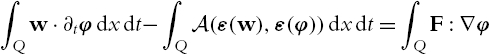
to
∫Qv⋅∂tφdxdt−∫QA(ε(v),ε(φ))dx=∫Qf⋅φdxdt

for all φ∈C∞0,div([0,T)×G)![]() such that ∇2v∈Lq(Q)
such that ∇2v∈Lq(Q)![]() . Moreover, we have
. Moreover, we have
∫Q|∇2v|qdxdt⩽c∫Q|f|qdxdt.

Proof
Due to the local Lq![]() -theory for the whole space problem and the half-space problem which follow from Corollary B.2.1 and Corollary B.2.2 (with the right scaling in T) the proof is similar to [133], Thm. 4.1, in the case A=I
-theory for the whole space problem and the half-space problem which follow from Corollary B.2.1 and Corollary B.2.2 (with the right scaling in T) the proof is similar to [133], Thm. 4.1, in the case A=I![]() . Note that Lq
. Note that Lq![]() -estimates for the stationary problem on bounded domains with given divergence are stated in Lemma B.1.1. We want to invert the operator
-estimates for the stationary problem on bounded domains with given divergence are stated in Lemma B.1.1. We want to invert the operator
L:Y→Lq(I;Lqdiv(G)),v↦Pq(∂tv−divAε(v)).

The space Y![]() is given by
is given by
Y:=Lq(I;W1,q0,div∩W2,q(G))∩W1,q(I;Lq(G))∩{v(0,⋅)=0,v∂G=0}
and Pq![]() is the Helmholtz projection from Lq(G)
is the Helmholtz projection from Lq(G)![]() into Lqdiv(G)
into Lqdiv(G)![]() . The latter one is defined by
. The latter one is defined by
Lqdiv(G):=‾C∞0,div(G)‖⋅‖q.
The Helmholtz-projection Pqu![]() of a function u∈Lq(G)
of a function u∈Lq(G)![]() can be defined as Pqu:=u−∇h
can be defined as Pqu:=u−∇h![]() , where h is the solution to the Neumann-problem
, where h is the solution to the Neumann-problem
{Δh=divuonG,NB⋅(∇h−u)=0on∂G.

We will try to find an operator R:Lq(I;Lqdiv(G))→Y![]() such that
such that
L∘R=I+τ
with ‖τ‖<1![]() . The range of L∘R
. The range of L∘R![]() (which then is Lq(0,T;Lqdiv(G))
(which then is Lq(0,T;Lqdiv(G))![]() ) is contained in the range of L
) is contained in the range of L![]() . So L
. So L![]() is onto.
is onto.
Let Gk![]() , 0=1,...,N
, 0=1,...,N![]() be a covering of G such that G0⋐G
be a covering of G such that G0⋐G![]() and Gk
and Gk![]() covers a (small) boundary strip of G. There are local coordinates
covers a (small) boundary strip of G. There are local coordinates
z=Zk(yk)=(yk1,yk2,yk3−Fk(yk1,yk2)),yk=(yk1,yk2)∈Bλ(ξk)
where Fk![]() is a C2
is a C2![]() -function and 0<λ⩽λ0<1
-function and 0<λ⩽λ0<1![]() . Here ξk
. Here ξk![]() denotes the center point of Sk=∂G∩Gk
denotes the center point of Sk=∂G∩Gk![]() and νk
and νk![]() the outer unit normal of Sk
the outer unit normal of Sk![]() at the point ξk
at the point ξk![]() . In this coordinate system we have a flat boundary which is contained in the plane {(x−ξk)⋅νk=0}
. In this coordinate system we have a flat boundary which is contained in the plane {(x−ξk)⋅νk=0}![]() . We consider a decomposition of unity (ζk)Nk=0⊂C∞0(R3)
. We consider a decomposition of unity (ζk)Nk=0⊂C∞0(R3)![]() with respect to Gk
with respect to Gk![]() such that sptζk⊂Gk
such that sptζk⊂Gk![]() . We can assume that |∇lζk|⩽cλ−l
. We can assume that |∇lζk|⩽cλ−l![]() for l=1,2
for l=1,2![]() and that the multiplicity of the covering of G by the domains Gk
and that the multiplicity of the covering of G by the domains Gk![]() does not depend on λ.
does not depend on λ.
Furthermore, M0f![]() and Mf
and Mf![]() is the extension of a function f (by zero) to the whole space or the half space respectively. Note that if f∈Lqdiv(G)
is the extension of a function f (by zero) to the whole space or the half space respectively. Note that if f∈Lqdiv(G)![]() , then M0f∈Lqdiv(R3)
, then M0f∈Lqdiv(R3)![]() . Finally, we denote by Ukf
. Finally, we denote by Ukf![]() (for f∈Lq(R3+)
(for f∈Lq(R3+)![]() ) and U0f
) and U0f![]() (for f∈Lq(R3)
(for f∈Lq(R3)![]() ) the solution on the half space (corresponding to the plane {(x−ξk)⋅νk=0}
) the solution on the half space (corresponding to the plane {(x−ξk)⋅νk=0}![]() ) and the whole space respectively (see Corollary B.2.1 and Corollary B.2.3). By Qkf
) and the whole space respectively (see Corollary B.2.1 and Corollary B.2.3). By Qkf![]() we denote the pressure corresponding to Ukf
we denote the pressure corresponding to Ukf![]() . Now we define the operators
. Now we define the operators
R0f:=ζ0U0M0f+N∑k=1ζkZ−1kUkMZkf,P0f:=N∑k=1Z−1kσQkMZkf.

The idea is in the interior to extend the force to the whole space, compute the whole space solution and localize again. At the boundary it is more tricky since we have to flatten the problem before considering the half space problem (and of course we have to transform back after solving it). Due to the involved cut-off functions R0f![]() is in general not divergence-free. This will be corrected in the following way: we set
is in general not divergence-free. This will be corrected in the following way: we set
Rf=R0f+R1f,Pf=P0f+P1f.
Here R1f=w![]() and P1f=s
and P1f=s![]() , where (w,s)
, where (w,s)![]() is the unique solution to the stationary problem
is the unique solution to the stationary problem
−divAε(w)+∇s=0,divw=divR0f,w|∂G=0,
cf. Lemma B.1.1. Now we clearly have Rf∈Y![]() . We need to establish (B.2.33). We abbreviate
. We need to establish (B.2.33). We abbreviate
uk:=Z−1kUkMZkf,πk:=Z−1kQkMZkf.

We define ˜∇k=∇x+Zk∇Fk∂z3![]() and accordingly ˜divk
and accordingly ˜divk![]() as well as ˜εk
as well as ˜εk![]() . We gain on QTk
. We gain on QTk![]()
∂tuk−˜divkA(˜εk(uk))+˜∇kπk=Z−1kZkf=f.
There holds
∂tRf−divAε(Rf)+∇Pf=f+Sf+∂tR1f,
Sf=−Aε(U0M0f)∇ζ0−divA(ζ0⊙U0M0f)−N∑k=1Aε(uk)∇ζk−N∑k=1divA(∇ζk⊙uk)+N∑k=1∇ζkπk−N∑k=1ζk(˜∇k−∇)πk+N∑k=1ζk(˜divkA(˜εk(⋅))−divA(ε(⋅)))uk.

From (B.2.34) it follows
LRf=f+PqSf+Pq∂tR1f
i.e. (B.2.33) with τ=PqS+Pq∂tR1![]() . We need to estimate the norms of the operators S
. We need to estimate the norms of the operators S![]() and ∂tR1
and ∂tR1![]() . If we choose T small enough the first two terms in (B.2.35) are small in accordance to Corollary B.2.1. The same is true for the first three sums as a consequence of Corollary B.2.3. All together we have
. If we choose T small enough the first two terms in (B.2.35) are small in accordance to Corollary B.2.1. The same is true for the first three sums as a consequence of Corollary B.2.3. All together we have
5∑i=1‖Ti‖q⩽δ(λ,T)‖f‖q

with δ(λ,T)→0![]() for T→0
for T→0![]() (and any fixed λ). Note that δ(λ,T)
(and any fixed λ). Note that δ(λ,T)![]() does not depend on N on account of the localization. We will argue similarly for the next three sums assuming that the gradients of the Fk
does not depend on N on account of the localization. We will argue similarly for the next three sums assuming that the gradients of the Fk![]() are small (meaning that λ is small). Here, we gain
are small (meaning that λ is small). Here, we gain
‖T6‖q+‖T7‖q⩽κ(λ)‖f‖q
with κ(λ)→0![]() for λ→0
for λ→0![]() . Note that κ(λ)
. Note that κ(λ)![]() does neither depend on T nor on N. By choosing first λ small enough such that κ(λ)⩽18
does neither depend on T nor on N. By choosing first λ small enough such that κ(λ)⩽18![]() and then T small enough such that δ(λ,T)⩽18
and then T small enough such that δ(λ,T)⩽18![]() we can follow
we can follow
‖Sf‖q⩽14‖f‖q.
Now we are going to show the same for ∂tR1![]() . In order to achieve this we consider the function w′=∂tR1f
. In order to achieve this we consider the function w′=∂tR1f![]() which is the solution to
which is the solution to
−divAε(∂tw′)+∇s′=0,divw′=div∂tR0f,w′|∂G=0.
We have the identity
div∂tR0f=N∑k=0∇ζk⋅∂tuk=N∑k=0˜∇kζk⋅∂tuk+N∑k=0(∇−˜∇k)ζk⋅∂tuk=N∑k=1˜∇kζk⋅(˜divkA(˜εk(uk))−˜∇kπk)+N∑k=0(˜∇k−∇)ζk⋅f+N∑k=1(∇−˜∇k)ζk⋅∂tuk=:T1+T2+T3,

where u0=U0M0f![]() and ˜∇0=∇
and ˜∇0=∇![]() . We use the formula
. We use the formula
T1=N∑k=1˜divk(˜∇kζkA(˜εk(uk))−˜∇kζkπk)−N∑k=1(˜∇2kζkA(˜εk(uk))−˜Δkζkπk)=:T11+T21,

as well as
(˜∇k−∇)gk=Zk∇Fk∂z3gk=Zk∂z3(∇Fkgk)=∂νk(Zk∇Fkgk)=νk⋅∇(Zk∇Fkgk)=div(νkZ−1k(∇Fkgk)).

Now we can apply Corollary B.1.1 with divg=T11![]() and g0=T21+T2+T3
and g0=T21+T2+T3![]() . By Corollary B.2.2 there are constants δ′(λ,T),δ″(λ,T)
. By Corollary B.2.2 there are constants δ′(λ,T),δ″(λ,T)![]() with δ′(λ,T)→0
with δ′(λ,T)→0![]() and δ″(λ,T)→0
and δ″(λ,T)→0![]() for T→0
for T→0![]() (and any fixed λ) such that
(and any fixed λ) such that
‖g‖q⩽δ′(λ,T)‖f‖q,‖g0‖q⩽c(1+δ″(λ,T))‖f‖q.
As a consequence of Corollary B.1.1 this yields
‖∂tR1f‖q⩽c(λβ+δ′(λ,T)+δ′(λ,T))‖f‖q.
Choosing first λ and then T small enough we gain
‖∂tR1f‖q⩽14‖f‖q.
Combining (B.2.36) and (B.2.37) implies ‖τ‖⩽12![]() . Hence L
. Hence L![]() is onto (recall (B.2.33)). This means we have shown the claim for T sufficiently small, say T=T0≪1
is onto (recall (B.2.33)). This means we have shown the claim for T sufficiently small, say T=T0≪1![]() . It is easy to extend it to the whole interval. Let (v,π)
. It is easy to extend it to the whole interval. Let (v,π)![]() be the solution on [0,T0]
be the solution on [0,T0]![]() . We extend it in an even manner to the interval [0,2T0]
. We extend it in an even manner to the interval [0,2T0]![]() . On the interval [T0,2T0]
. On the interval [T0,2T0]![]() we define (v′,π′)
we define (v′,π′)![]() as solution to the A
as solution to the A![]() -Stokes system with right-hand-side
-Stokes system with right-hand-side
f′(t,x)=f(t,x)−f(x,2T0−t)+2∂tv(x,2T0−t).
If we set v′=0,π′=0![]() on [0,T0]
on [0,T0]![]() then (v+v′,π+π′)
then (v+v′,π+π′)![]() is the solution on [0,2T0]
is the solution on [0,2T0]![]() . This can be repeated to construct the solution on [0,T]
. This can be repeated to construct the solution on [0,T]![]() . □
. □
B.3 The non-stationary problem in divergence form
In order to treat problems with right hand side in divergence form we consider the A![]() -Stokes operator
-Stokes operator
Aq:=−PqdivA(ε(⋅)).
The A![]() -Stokes operator Aq
-Stokes operator Aq![]() enjoys the same properties than the Stokes operator Aq
enjoys the same properties than the Stokes operator Aq![]() (see for instance [87]).
(see for instance [87]).
For the A![]() -Stokes operator it holds D(Aq)=W1,q0,div∩W2,q(G)
-Stokes operator it holds D(Aq)=W1,q0,div∩W2,q(G)![]() , where D denotes the domain, and
, where D denotes the domain, and
‖u‖2,q⩽c1‖Aqu‖q⩽c2‖u‖2,q,u∈D(Aq),
∫GAqu⋅wdx=∫Gu⋅Aq′wdxu∈D(Aq),w∈D(Aq′).

Inequality (B.3.38) is a consequence of Lemma B.1.1 a) and the continuity of Pq![]() .
.
Since Aq![]() is positive its root A12q
is positive its root A12q![]() is well-defined with D(A12q)=W1,q0,div(G)
is well-defined with D(A12q)=W1,q0,div(G)![]() and
and
‖u‖1,q⩽c1‖A12qu‖q⩽c2‖u‖1,q,u∈D(A12q),
∫GA12qu⋅wdx=∫Gu⋅A12q′wdxu∈D(A12q),w∈D(A12q′).

Finally, the inverse operator A−12q:Lqdiv(G)→W1,q0,div(G)![]() is defined and it holds
is defined and it holds
‖∇A−12qu‖q⩽c‖u‖q,u∈D(A−12q),
∫GA−12qu⋅wdx=∫Gu⋅A−12q′wdxu∈D(A−12q),w∈D(A−12q′).

From the definition of the square root of a positive self-adjoint operator follows also that
A12q′:W2,q′∩W1,q′0,div(G)→W1,q′0,div(G),A−12q′:W1,q′0,div(G)→W2,q′∩W1,q′0,div(G),

together with
‖∇A12qu‖q⩽c‖u‖2,q,u∈W2,q′∩W1,q′0,div(G),
‖∇A−12qu‖q⩽c‖u‖q,u∈W1,q′0,div(G).
Finally we state the main result of this section.
Theorem B.3.50

Proof
Let us first assume that q>2![]() . Then Theorem B.2.49 applies. We set f:=A−12qdivF
. Then Theorem B.2.49 applies. We set f:=A−12qdivF![]() which is defined via the duality
which is defined via the duality
∫GA−12qdivF⋅φdx=∫GF:∇A−12q′φdx,φ∈C∞0,div(G),

using (B.3.43). So we gain f∈Lqdiv(G)![]() with
with
‖f‖q⩽c‖F‖q.
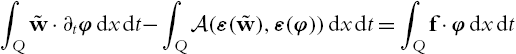
We define ˜w∈Lq(0,T;W1,q0,div(G))![]() as the unique solution to
as the unique solution to
∫Q˜w⋅∂tφdxdt−∫QA(ε(˜w),ε(φ))dxdt=∫Qf⋅φdxdt
for all φ∈C∞0,div([0,T)×G)![]() . Theorem B.2.49 yields ˜w∈Lq(0,T;W2,q(G))
. Theorem B.2.49 yields ˜w∈Lq(0,T;W2,q(G))![]() and
and
‖˜w‖2,q⩽c‖f‖q.
We want to return to the original problem and set w:=A12q˜w![]() thus we have w∈Lq(0,T;W1,q0,div(G))
thus we have w∈Lq(0,T;W1,q0,div(G))![]() . Since A12q′:W1,q′0,div∩W2,q′(G)→W1,q′0,div(G)
. Since A12q′:W1,q′0,div∩W2,q′(G)→W1,q′0,div(G)![]() we can replace φ by A12q′φ
we can replace φ by A12q′φ![]() in (B.3.48). This implies using (B.3.41) and the definition of f
in (B.3.48). This implies using (B.3.41) and the definition of f
∫Qw⋅∂tφdxdt+∫QdivA(ε(˜w)):A12q′φdxdt=∫QF:∇φ

for all φ∈C∞0,div(Q)![]() . On account of A12q′φ∈W1,q′0,div(G)
. On account of A12q′φ∈W1,q′0,div(G)![]() and A12q˜w∈W1,q0,div(G)
and A12q˜w∈W1,q0,div(G)![]() we gain due to (B.3.41)
we gain due to (B.3.41)
∫QdivA(ε(˜w)):A12q′φdxdt=∫QAq˜w:A12q′φdxdt=∫QA12q˜w:Aq′φdxdt=∫Qw⋅divA(ε(φ))dxdt=−∫QA(ε(w),ε(φ))dxdt

using (B.3.41) and w∈W1,q0,div(G)![]() . This shows that w is the unique solution to (6.2.27). Moreover, we obtain the desired regularity estimate via
. This shows that w is the unique solution to (6.2.27). Moreover, we obtain the desired regularity estimate via
∫Q|∇w|qdxdt⩽c∫Q|A12qw|qdxdt=c∫Q|Aq˜w|qdxdt⩽c∫Q|∇2˜w|q⩽c∫Q|f|qdxdt⩽c∫Q|F|qdxdt
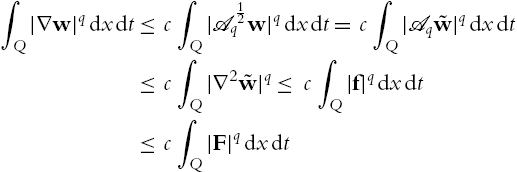
as a consequence of (B.3.40), the definition of w, (B.3.38), (B.3.49), and (B.3.47). A simple scaling argument shows that the inequality is independent of the diameter of I and B. So we have shown the claim for q>2![]() .
.
The case q=2![]() follows easily from a priori estimates and Korn's inequality. So let us assume that q<2
follows easily from a priori estimates and Korn's inequality. So let us assume that q<2![]() . Duality arguments show that
. Duality arguments show that
1q⨍Q|∇w|qdxdt=supG∈Lq′(Q)[⨍Q∇w:Gdxdt−1q′⨍Q|G|q′dxdt].

For a given G∈Lq′(Q)![]() let zG
let zG![]() be the unique Lq′(0,T;W1,q′0,div(G))
be the unique Lq′(0,T;W1,q′0,div(G))![]() -solution to
-solution to
⨍Qz⋅∂tξdxdt+∫QA(ε(z),ε(ξ))dxdt=∫QG:∇ξdxdt

for all ξ∈C∞0,div((0,T]×G)![]() . This is a backward parabolic equation with end datum zero. We have that ∂tzG∈Lq′(0,T;W−1,q′div(G))
. This is a backward parabolic equation with end datum zero. We have that ∂tzG∈Lq′(0,T;W−1,q′div(G))![]() such that test-functions can be chosen from the space Lq(0,T;W1,q0,div(G))
such that test-functions can be chosen from the space Lq(0,T;W1,q0,div(G))![]() . Due to q′>2
. Due to q′>2![]() the first part of the proof (applied to ˜z˜G(t,⋅)=zG(T−t,⋅)
the first part of the proof (applied to ˜z˜G(t,⋅)=zG(T−t,⋅)![]() , where ˜G(t,⋅)=G(T−t,⋅)
, where ˜G(t,⋅)=G(T−t,⋅)![]() ) yields
) yields
⨍Q|∇zG|q′dxdt⩽c⨍Q|G|q′dxdt.

This and w(0,⋅)=0![]() implies (using w as a test-function in (B.3.50))
implies (using w as a test-function in (B.3.50))
⨍Q|∇w|qdxdt⩽csupG∈Lq′(Q)[⨍QA(ε(w),ε(zG))dxdt−⨍Q∂tzG⋅wdxdt−⨍Q|∇zG|q′dxdt]⩽csupξ∈C∞0,div(Q)[⨍QA(ε(w),ε(ξ))dxdt−⨍Qw⋅∂tξdxdt−⨍Q|∇ξ|q′dxdt].

The equation for w and Young's inequality finally give
⨍Q|∇w|qdxdt⩽csupξ∈C∞0,div(Q)[⨍QF:∇ξdxdt−⨍Q|∇ξ|q′dxdt]⩽c⨍Q|F|qdxdt

and hence the claim. □