
Preliminaries
Abstract
In this chapter we present some preliminary material which will be needed in order to study stationary models for generalized Newtonian fluids. We begin with the functional analytic framework. In particular, we define Lebesgue-, Sobolev- and Orlicz-spaces and describe their basic properties. After this we present the Lipschitz truncation method in its classical framework and present two applications. Finally, we discuss some modelling aspects concerning power law fluids and provide a historical overview on the mathematical theory of weak solutions for stationary flows.
Keywords
Lebesgue spaces; Sobolev spaces; Orlicz spaces; Lipschitz truncation; Stationary generalized Newtonian fluids; Historical comments on existence theory
1.1 Lebesgue & Sobolev spaces
In this section we define various function spaces. For proofs, further details and references we refer to [5].
Definition 1.1.1
Classical function spaces

Remark 1.1.1
In Definition 1.1.1 if we replace G by the closed set ‾G![]() we are considering functions whose derivatives are continuous up to the boundary of G.
we are considering functions whose derivatives are continuous up to the boundary of G.
Definition 1.1.2

Remark 1.1.2
In the case α=1![]() we obtain the set of Lipschitz continuous functions.
we obtain the set of Lipschitz continuous functions.
Definition 1.1.3
Definition 1.1.4
Lebesgue spaces
Let (X,Σ,μ)![]() be a measure space. We define
be a measure space. We define
Lp(X,Σ,μ):={u:X→R:u is μ-measurable,∫X|u|pdμ<∞},1⩽p<∞,L∞(X,Σ,μ):={u:X→R:u is μ-measurable,infμ(N)=0supx∈X∖N|u(x)|<∞}.

The elements of Lp(X,Σ,μ)![]() are equivalence classes. Two functions u and v belong to the same equivalence class if u=v
are equivalence classes. Two functions u and v belong to the same equivalence class if u=v![]() μ-almost everywhere in X
μ-almost everywhere in X![]() , i.e. if
, i.e. if
μ{x∈X:u(x)≠v(x)}=0.
Remark 1.1.3
• Lp(X,Σ,μ)![]() is a Banach space together with the natural norm
is a Banach space together with the natural norm
‖u‖p:=‖u‖Lp(X):=(∫X|u|pdμ)1pfor1⩽p<∞,‖u‖∞:=‖u‖L∞(X):=infμ(N)=0supx∈X∖N|u(x)|.

• We set p′=pp−1![]() for 1<p<∞
for 1<p<∞![]() , p′=∞
, p′=∞![]() for p=1
for p=1![]() and p′=1
and p′=1![]() for p=∞
for p=∞![]() . Let 1⩽p<∞
. Let 1⩽p<∞![]() and v∈Lp′(X,Σ,μ)
and v∈Lp′(X,Σ,μ)![]() . Then the mapping
. Then the mapping
Lp(X,Σ,μ)∋u↦∫Guvdμ

belongs to the dual space Lp(X,Σ,μ)′![]() . On the other hand each element of Lp(X,Σ,μ)′
. On the other hand each element of Lp(X,Σ,μ)′![]() can be represented via a function v∈Lp′(X,Σ,μ)
can be represented via a function v∈Lp′(X,Σ,μ)![]() . In particular, the mapping
. In particular, the mapping
Lp′(X,Σ,μ)∋v↦(Lp(X,Σ,μ)∋u↦∫Xuvdμ)∈Lp(X,Σ,μ)′

is an isomorphism.
• The space Lp(X,Σ,μ)![]() is reflexive if and only if 1<p<∞
is reflexive if and only if 1<p<∞![]() .
.
• If μ(X)<∞![]() we have that Lq(X,Σ,μ)⊂Lp(X,Σ,μ)
we have that Lq(X,Σ,μ)⊂Lp(X,Σ,μ)![]() for 1⩽p⩽q⩽∞
for 1⩽p⩽q⩽∞![]() . In particular, the following holds
. In particular, the following holds
‖u‖Lp(X)⩽c(d,p,q,μ(X))‖u‖Lq(X)
for every u∈Lq(X,Σ,μ)![]() .
.
• We can define vector- or matrix-valued Lp![]() -spaces component-wise. For simplicity we do not mention this in the notation. However, when considering functions with values in an infinite dimensional spaces X we denote this by writing Lp(X,Σ,μ;X)
-spaces component-wise. For simplicity we do not mention this in the notation. However, when considering functions with values in an infinite dimensional spaces X we denote this by writing Lp(X,Σ,μ;X)![]() .
.
The most important special case is (X,Σ,μ)=(G,B(Rd),Ld)![]() where G⊂Rd
where G⊂Rd![]() , B(Rd)
, B(Rd)![]() is the Borel σ-algebra on Rd
is the Borel σ-algebra on Rd![]() and Ld
and Ld![]() the d-dimensional Lebesgue measure. In this case we abbreviate the notation by setting Lp(G):=Lp(G,B(Rd),Ld)
the d-dimensional Lebesgue measure. In this case we abbreviate the notation by setting Lp(G):=Lp(G,B(Rd),Ld)![]() . If 1⩽p<∞
. If 1⩽p<∞![]() then C∞0(G)
then C∞0(G)![]() is dense in Lp(G)
is dense in Lp(G)![]() . In particular, for every u∈Lp(G)
. In particular, for every u∈Lp(G)![]() there is (um)⊂C∞0(G)
there is (um)⊂C∞0(G)![]() such that um→u
such that um→u![]() in Lp(G)
in Lp(G)![]() .
.
Definition 1.1.5
Local Lebesgue spaces
Definition 1.1.6
Weak derivative
Let G⊂Rd![]() be open and u∈L1loc(G)
be open and u∈L1loc(G)![]() .
.
• u is called weakly differentiable with respect to the i-th variable if there is a function vi∈L1loc(G)![]() such that
such that
∫Gu∂iφdz=−∫Gviφdzfor allφ∈C∞0(G).

We call vi![]() the weak derivative of u with respect to the i-th variable. If weak derivatives with respect to all variables exist, we call u weakly differentiable and denote by ∇u=(v1,...,vn)
the weak derivative of u with respect to the i-th variable. If weak derivatives with respect to all variables exist, we call u weakly differentiable and denote by ∇u=(v1,...,vn)![]() the weak gradient of u.
the weak gradient of u.
• Let α∈Nd0![]() and |α|:=α1+...+αn
and |α|:=α1+...+αn![]() . For a smooth function u we denote by Dαu:=∂|α|u∂α1x1...∂αnxn
. For a smooth function u we denote by Dαu:=∂|α|u∂α1x1...∂αnxn![]() its α-th classical derivative. A function u∈L1loc(G)
its α-th classical derivative. A function u∈L1loc(G)![]() is called k-times weakly differentiable if for all α∈Nd0
is called k-times weakly differentiable if for all α∈Nd0![]() with |α|⩽k
with |α|⩽k![]() there is a function vα∈L1loc(G)
there is a function vα∈L1loc(G)![]() such that
such that
∫GuDαφdz=(−1)|α|∫Gvαφdzfor allφ∈C∞0(G).

We call Dαu=vα![]() the α-th weak derivative.
the α-th weak derivative.
Definition 1.1.7
Sobolev spaces

Remark 1.1.4
• Wk,p(G)![]() (1⩽p⩽∞
(1⩽p⩽∞![]() ) is a Banach space together with the norm
) is a Banach space together with the norm
‖u‖k,p:=‖u‖Wk,p(G):=(∑|α|⩽k∫G|Dαu|pdz)1pfor1⩽p<∞,‖u‖k,∞:=‖u‖Wk,∞(G):=∑|α|⩽kinfLd(N)=0supx∈G∖N|Dαu(x)|.

• The space Wk,p(G)![]() is reflexive iff 1<p<∞
is reflexive iff 1<p<∞![]() .
.
• A sequence (uk)⊂Wk,p(G)![]() (1<p<∞
(1<p<∞![]() ) converges weakly to u in Wk,p(G)
) converges weakly to u in Wk,p(G)![]() if
if
∫GDαukvdz⟶∫GDαuvdz,k→∞,

for all v∈Lp′(G,RN)![]() (p′:=pp−1
(p′:=pp−1![]() ) and for all α∈Nd0
) and for all α∈Nd0![]() with |α|⩽k
with |α|⩽k![]() .
.
• The dual space of Wk,p0(G)![]() will be denoted by W−k,p′(G)
will be denoted by W−k,p′(G)![]() .
.
Theorem 1.1.1
Smooth approximation
Let G⊂Rd![]() be open and bounded with Lipschitz boundary (i.e. ∂Ω can be locally parametrized by Lipschitz continuous functions of d−1
be open and bounded with Lipschitz boundary (i.e. ∂Ω can be locally parametrized by Lipschitz continuous functions of d−1![]() variables) and 1⩽p<∞
variables) and 1⩽p<∞![]() . Then C∞(‾G)
. Then C∞(‾G)![]() is dense in Wk,p(G)
is dense in Wk,p(G)![]() . In particular, for every u∈Wk,p(G)
. In particular, for every u∈Wk,p(G)![]() there is (um)⊂C∞0(G)
there is (um)⊂C∞0(G)![]() such that um→u
such that um→u![]() in Wk,p(G)
in Wk,p(G)![]() .
.
Theorem 1.1.2
Sobolev


Theorem 1.1.3
Kondrachov
In Definition 1.1.7 we have interpreted the boundary values of a Sobolev function as follows: u=0![]() on ∂G iff u∈W1,p0(G)
on ∂G iff u∈W1,p0(G)![]() , where W1,p0(G)
, where W1,p0(G)![]() for p<∞
for p<∞![]() denotes the closure of C∞0(G)
denotes the closure of C∞0(G)![]() in W1,p(G)
in W1,p(G)![]() . We will develop a rigorous definition of boundary values and show that it coincides with the former one. In order to do so we need functions which are integrable over the boundary of G. For G⊂Rd
. We will develop a rigorous definition of boundary values and show that it coincides with the former one. In order to do so we need functions which are integrable over the boundary of G. For G⊂Rd![]() open let Lp(∂G)
open let Lp(∂G)![]() be equal to the set of all Hd−1
be equal to the set of all Hd−1![]() -measurable functions with
-measurable functions with
‖u‖Lp(∂Ω):=(∫∂G|u|pdHd−1)1p<∞.

Here Hd−1![]() denotes the (d−1)
denotes the (d−1)![]() -dimensional Hausdorff measure. For C1
-dimensional Hausdorff measure. For C1![]() -functions we define the operator tr:C1(‾G)→Lp(∂G)
-functions we define the operator tr:C1(‾G)→Lp(∂G)![]() by tru:=u|∂G
by tru:=u|∂G![]() .
.
Lemma 1.1.1
For u∈W1,p(G)![]() we consider the approximation sequence um∈C∞(‾G)
we consider the approximation sequence um∈C∞(‾G)![]() with ‖um−u‖1,p→0
with ‖um−u‖1,p→0![]() . Its existence follows from Theorem 1.1.1. Lemma 1.1.1 shows that (trum)
. Its existence follows from Theorem 1.1.1. Lemma 1.1.1 shows that (trum)![]() is a Cauchy-sequence in Lp(∂G)
is a Cauchy-sequence in Lp(∂G)![]() . We define its limit (which does not depend on the special choice of the sequence) as the trace of u. The result is a linear operator tr:W1,p(G)→Lp(∂G)
. We define its limit (which does not depend on the special choice of the sequence) as the trace of u. The result is a linear operator tr:W1,p(G)→Lp(∂G)![]() which coincides with the classical trace operator on C1(‾G)
which coincides with the classical trace operator on C1(‾G)![]() .
.
Theorem 1.1.4
All results of this section generalize in a straightforward manner to spaces of vector-valued functions. In order to keep the notation simple we do not use target spaces in the notation for our function spaces. It will follow from the context (and the bold-symbol) when we are dealing with these. In fluid mechanics the velocity field is a function from Rd⊃G→Rd![]() . In this setting we need function spaces of solenoidal (that is, divergence-free) functions. We will use the following notation for 1⩽p<∞
. In this setting we need function spaces of solenoidal (that is, divergence-free) functions. We will use the following notation for 1⩽p<∞![]()
W1,pdiv(G):={ψ∈W1,p(G):divψ=0},C∞0,div(Ω):={ψ∈C∞0(G):divψ=0},Lpdiv(G):=‾C∞0,div(G)L2(G),W1,p0,div(G):=‾C∞0,div(G)W1,p(G).

Finally we write W−1,p′div(G)![]() for the dual of W1,p0,div(G)
for the dual of W1,p0,div(G)![]() .
.
1.2 Orlicz spaces
In this section we present some important properties of Orlicz spaces (see [125] and [5]).
A function A:[0,∞)→[0,∞]![]() is called a Young function if it is convex, left-continuous, vanishing at 0, and neither identically equal to 0 nor to ∞. Thus, with any such function, it is uniquely associated a (non-trivial) non-decreasing left-continuous function a:[0,∞)→[0,∞]
is called a Young function if it is convex, left-continuous, vanishing at 0, and neither identically equal to 0 nor to ∞. Thus, with any such function, it is uniquely associated a (non-trivial) non-decreasing left-continuous function a:[0,∞)→[0,∞]![]() such that
such that
A(s)=∫s0a(r)drfors⩾0.

The Young conjugate ˜A![]() of A is the Young function defined by
of A is the Young function defined by
˜A(s)=sup{rs−A(r):r⩾0}fors⩾0.
For ˜A![]() we have the representation formula
we have the representation formula
˜A(s)=∫s0a−1(r)drfors⩾0,

where a−1![]() denotes the (generalized) left-continuous inverse of a. Moreover, for every Young function A,
denotes the (generalized) left-continuous inverse of a. Moreover, for every Young function A,
r⩽A−1(r)˜A−1(r)⩽2rforr⩾0
as well as
˜˜A=A.
Let A be a Young function of the form (1.2.1). Then the convexity of A and A(0)=0![]() imply
imply
A(λs)⩽λA(s)for allλ∈[0,1]
and all s⩾0![]() . If λ⩾1
. If λ⩾1![]() , then
, then
λA(s)⩽A(λs)fors⩾0.
As a consequence, if λ⩾1![]() , then
, then
A−1(λs)⩽λA−1(s)fors⩾0,
where A−1![]() denotes the (generalized) right-continuous inverse of A.
denotes the (generalized) right-continuous inverse of A.
A Young function A is said to satisfy the Δ2![]() -condition if there exists a positive constant K such that
-condition if there exists a positive constant K such that
A(2s)⩽KA(s)fors⩾0.
If (1.2.8) just holds for s⩾s0![]() for some s0>0
for some s0>0![]() , then A is said to satisfy the Δ2
, then A is said to satisfy the Δ2![]() -condition near infinity. We say that A satisfies the ∇2
-condition near infinity. We say that A satisfies the ∇2![]() -condition [near infinity] if ˜A
-condition [near infinity] if ˜A![]() satisfies the Δ2
satisfies the Δ2![]() -condition [near infinity].
-condition [near infinity].
A Young function A is said to dominate another Young function B near infinity if there exist positive constants c and s0![]() such that
such that
B(s)⩽A(cs)fors⩾s0.
The functions A and B are called equivalent near infinity if they dominate each other near infinity.
Let G be a measurable subset of Rd![]() , and let u:G→R
, and let u:G→R![]() be a measurable function. Given a Young function A, the Luxemburg norm associated with A, of the function u is defined as
be a measurable function. Given a Young function A, the Luxemburg norm associated with A, of the function u is defined as
‖u‖LA(G):=inf{λ:∫GA(|u|λ)dx⩽1}.

The collection of all measurable functions u for which this norm is finite is called the Orlicz space LA(G)![]() . It turns out to be Banach function space. The subspace of LA(G)
. It turns out to be Banach function space. The subspace of LA(G)![]() of those functions u such that ∫Gu(x)dx=0
of those functions u such that ∫Gu(x)dx=0![]() will be denoted by LA⊥(G)
will be denoted by LA⊥(G)![]() . A Hölder-type inequality in Orlicz spaces takes the form
. A Hölder-type inequality in Orlicz spaces takes the form
‖v‖L˜A(G)⩽supu∈LA(G)∫Gu(x)v(x)dx‖u‖LA(G)⩽2‖v‖L˜A(G)

for every v∈L˜A(G)![]() . If |G|<∞
. If |G|<∞![]() , then
, then
LA(G)↪LB(G)if and only if A dominates B near infinity.
The decreasing rearrangement u⁎:[0,∞)→[0,∞]![]() of a measurable function u:G→R
of a measurable function u:G→R![]() is the (unique) non-increasing, right-continuous function which is equimeasurable with u. Thus,
is the (unique) non-increasing, right-continuous function which is equimeasurable with u. Thus,
u⁎(s)=sup{t⩾0:|{x∈G:|u(x)|>t}|>s}fors⩾0.
The equimeasurability of u and u⁎![]() implies that
implies that
‖u‖LA(G)=‖u⁎‖LA(0,|G|)
for every u∈LA(G)![]() .
.
The Lebesgue spaces Lp(G)![]() , corresponding to the choice Ap(t)=tp
, corresponding to the choice Ap(t)=tp![]() , if p∈[1,∞)
, if p∈[1,∞)![]() , and A∞(t)=∞⋅χ(1,∞)(t)
, and A∞(t)=∞⋅χ(1,∞)(t)![]() , if p=∞
, if p=∞![]() , are a basic example of Orlicz spaces. Other instances of Orlicz spaces are provided by the Zygmund spaces LplogαL(G)
, are a basic example of Orlicz spaces. Other instances of Orlicz spaces are provided by the Zygmund spaces LplogαL(G)![]() , and by the exponential spaces expLβ(G)
, and by the exponential spaces expLβ(G)![]() . If either p>1
. If either p>1![]() and α∈R
and α∈R![]() , or p=1
, or p=1![]() and α⩾0
and α⩾0![]() , then LplogαL(G)
, then LplogαL(G)![]() is the Orlicz space associated with a Young function equivalent to tp(logt)α
is the Orlicz space associated with a Young function equivalent to tp(logt)α![]() near infinity. Given β>0
near infinity. Given β>0![]() , expLβ(G)
, expLβ(G)![]() denotes the Orlicz space built upon a Young function equivalent to etβ
denotes the Orlicz space built upon a Young function equivalent to etβ![]() near infinity.
near infinity.
An important tool will be the following characterization of Hardy type inequalities in Orlicz spaces [46, Lemma 1].
Lemma 1.2.1
Let A and B be Young functions, and let L∈(0,∞]![]() .
.
(i) There exists a constant C such that
‖1s∫s0f(r)dr‖LB(0,L)⩽C‖f‖LA(0,L)
for every f∈LA(0,L)![]() if and only if either L<∞
if and only if either L<∞![]() and there exist constants c>0
and there exist constants c>0![]() and t0⩾0
and t0⩾0![]() such that
such that
t∫tt0B(s)s2ds⩽A(ct)for t⩾t0,

or L=∞![]() and (1.2.14) holds with t0=0
and (1.2.14) holds with t0=0![]() . In particular, in the latter case, the constant C in (1.2.13) depends only on the constant c appearing in (7.0.1).
. In particular, in the latter case, the constant C in (1.2.13) depends only on the constant c appearing in (7.0.1).
(ii) There exists a constant C such that
‖∫Lsf(r)drr‖LB(0,L)⩽C‖f‖LA(0,L)

for every f∈LA(0,L)![]() if and only if either L<∞
if and only if either L<∞![]() and there exist constants c>0
and there exist constants c>0![]() and t0⩾0
and t0⩾0![]() such that
such that
t∫tt0˜A(s)s2ds⩽˜B(ct)for t⩾t0,
or L=∞![]() and (1.2.16) holds with t0=0
and (1.2.16) holds with t0=0![]() . In particular, in the latter case, the constant C in (1.2.15) depends only on the constant c appearing in (1.2.16).
. In particular, in the latter case, the constant C in (1.2.15) depends only on the constant c appearing in (1.2.16).
Assume now that G is an open set. The Orlicz–Sobolev space W1,A(G)![]() is the set of all functions in LA(G)
is the set of all functions in LA(G)![]() whose distributional gradient also belongs to LA(G)
whose distributional gradient also belongs to LA(G)![]() . It is a Banach space endowed with the norm
. It is a Banach space endowed with the norm
‖u‖W1,A(G):=‖u‖LA(G)+‖∇u‖LA(G).
We also define the subspace of W1,A(G)![]() of those functions which vanish on ∂G as
of those functions which vanish on ∂G as
W1,A0(G)={u∈W1,A(G):the continuation of u by 0 is weakly differentiable}.

In the case where A(t)=tp![]() for some p⩾1
for some p⩾1![]() , and ∂G is regular enough, such a definition of W1,A0(G)
, and ∂G is regular enough, such a definition of W1,A0(G)![]() can be shown to reproduce the usual space W1,p0(G)
can be shown to reproduce the usual space W1,p0(G)![]() defined as the closure in W1,p(G)
defined as the closure in W1,p(G)![]() of the space C∞0(G)
of the space C∞0(G)![]() of smooth compactly supported functions in G. In general, the set of smooth bounded functions is dense in LA(G)
of smooth compactly supported functions in G. In general, the set of smooth bounded functions is dense in LA(G)![]() only if A satisfies the Δ2
only if A satisfies the Δ2![]() -condition (just near infinity when |G|<∞
-condition (just near infinity when |G|<∞![]() ), and hence, for arbitrary A, our definition of W1,A0(G)
), and hence, for arbitrary A, our definition of W1,A0(G)![]() yields a space which can be larger than the closure of C∞0(G)
yields a space which can be larger than the closure of C∞0(G)![]() in W1,A0(G)
in W1,A0(G)![]() even for smooth domains. On the other hand, if G is a Lipschitz domain, namely a bounded open set in Rd
even for smooth domains. On the other hand, if G is a Lipschitz domain, namely a bounded open set in Rd![]() which is locally the graph of a Lipschitz function of d−1
which is locally the graph of a Lipschitz function of d−1![]() variables, then
variables, then
W1,A0(G)=W1,A(G)∩W1,10(G),
where W1,10(G)![]() is defined as usual.
is defined as usual.
Lemma 1.2.2
Lemma 1.2.3
1.3 Basics on Lipschitz truncation
The purpose of the Lipschitz truncation technique is to approximate a Sobolev function u∈W1,p![]() by λ-Lipschitz functions uλ
by λ-Lipschitz functions uλ![]() that coincide with u up to a set of small measure. The functions uλ
that coincide with u up to a set of small measure. The functions uλ![]() are constructed nonlinearly by modifying u on the level set of the Hardy–Littlewood maximal function of the gradient ∇u. This idea goes back to Acerbi and Fusco [1–3]. Lipschitz truncations are used in various areas of analysis: calculus of variations, in the existence theory of partial differential equations, and in regularity theory. We refer to [62] for a longer list of references.
are constructed nonlinearly by modifying u on the level set of the Hardy–Littlewood maximal function of the gradient ∇u. This idea goes back to Acerbi and Fusco [1–3]. Lipschitz truncations are used in various areas of analysis: calculus of variations, in the existence theory of partial differential equations, and in regularity theory. We refer to [62] for a longer list of references.
The basic idea is to take a function u∈W1,p(Rd)![]() , where p⩾1
, where p⩾1![]() , and cut values where the maximal function of its gradient is large. The Hardy–Littlewood maximal operator is defined by
, and cut values where the maximal function of its gradient is large. The Hardy–Littlewood maximal operator is defined by
M(v)(x)=supB:x∈B⨍B|v|dy
for v∈L1loc(Rd)![]() which can be extended to vector- (or matrix-)valued functions by setting M(v)=M(|v|)
which can be extended to vector- (or matrix-)valued functions by setting M(v)=M(|v|)![]() . Basic properties of the maximal operator are summarized in the following lemma (see e.g. [134] and [141, Lemma 3.2] for d)).
. Basic properties of the maximal operator are summarized in the following lemma (see e.g. [134] and [141, Lemma 3.2] for d)).
Lemma 1.3.1
a) Let v∈L1loc(Rd)![]() and λ>0
and λ>0![]() . The level-set {x∈Rd:|M(v)(x)|>λ}
. The level-set {x∈Rd:|M(v)(x)|>λ}![]() is open.
is open.
b) The strong-type estimate
‖M(v)‖Lp(Rd)⩽cp‖v‖Lp(Rd)∀v∈Lp(Rd)
holds for all p∈(1,∞]![]() .
.
c) The weak-type estimate
Ld({x∈Rd:|M(v)(x)|>λ})⩽cp‖v‖ppλp∀v∈Lp(Rd)

holds for all p∈[1,∞)![]() and all λ>0
and all λ>0![]() .
.
d) We have the estimate
∫{M(v)>λ}|v|pdx⩽cp∫{|v|>λ/2}|v|pdx∀p∈[1,∞)

for all λ>0![]() .
.
The Lipschitz truncation will be defined via the maximal function of the gradient. For u∈W1,p(Rd)![]() the “bad set” is defined by
the “bad set” is defined by
Oλ:={x∈Rd:M(∇u)(x)>λ},
where λ⩾0![]() . If we have u∈W1,p(G)
. If we have u∈W1,p(G)![]() for G≠Rd
for G≠Rd![]() it has to be extended to u∈W1,p(Rd)
it has to be extended to u∈W1,p(Rd)![]() . This can be done in an obvious way if u∈W1,p0(G)
. This can be done in an obvious way if u∈W1,p0(G)![]() where the extension is zero outside G. In the general case we may apply [5, Thm. 4.26]. Now, for x,y∈Rd∖Oλ
where the extension is zero outside G. In the general case we may apply [5, Thm. 4.26]. Now, for x,y∈Rd∖Oλ![]() we have a.e.
we have a.e.
|u(x)−u(y)|⩽c|x−y|(M(∇u)(x)+M(∇u)(y))⩽2cλ|x−y|,
see, e.g., [112]. Hence u is Lipschitz-continuous in Rd∖Oλ![]() with Lipschitz constant proportional to λ. By a standard extension theorem (see e.g. [71, p. 201]) we can extend u (defined in Rd∖Oλ
with Lipschitz constant proportional to λ. By a standard extension theorem (see e.g. [71, p. 201]) we can extend u (defined in Rd∖Oλ![]() ) to uλ
) to uλ![]() (defined in Rd
(defined in Rd![]() ) such that the Lipschitz constant is preserved. (When dealing with this simple extension it is necessary to cut large values of M(u)
) such that the Lipschitz constant is preserved. (When dealing with this simple extension it is necessary to cut large values of M(u)![]() as well. We neglect this for brevity.) This means we have
as well. We neglect this for brevity.) This means we have
|∇uλ|⩽cλinRd.
Moreover, by construction we have
{x∈Rd:u≠uλ}⊂Oλ.
This and Lemma 1.3.1 c) imply
Ld({x∈Rd:u≠uλ})⩽Ld(Oλ)⩽c‖∇u‖ppλp.

Combining (1.3.18) and (1.3.19) shows
∫Rd|∇uλ|pdx=∫Rd∖Oλ|∇uλ|pdx+∫Oλ|∇uλ|pdx⩽∫Rd∖Oλ|∇u|pdx+cλpLd(Oλ)⩽c∫Rd|∇u|pdx.

We obtain the following stability result
‖∇uλ‖p⩽c‖∇u‖p.
The basic properties (1.3.18)–(1.3.20) are already enough to make the Lipschitz truncation a powerful tool for numerous applications. We present two rather classical ones.
Lower semi-continuity in W1,p![]() .
.
Let G⊂Rd![]() be an open and bounded with Lipschitz boundary. Suppose further that F:G×Rd×D→[0,∞)
be an open and bounded with Lipschitz boundary. Suppose further that F:G×Rd×D→[0,∞)![]() is a continuous function with p-growth (p>1
is a continuous function with p-growth (p>1![]() ), i.e.,
), i.e.,
F(x,Q)⩽c|Q|p+g(x)∀Q∈Rd×D
with a constant c⩾0![]() and a non-negative function g∈L1(G)
and a non-negative function g∈L1(G)![]() . We are interested in minimizing the functional
. We are interested in minimizing the functional
GF[w]=∫GF(x,∇w)dx

defined for functions w:G→RD![]() . An important concept in showing the existence of minimizers is the lower semi-continuity of GF
. An important concept in showing the existence of minimizers is the lower semi-continuity of GF![]() with respect to an appropriate topology. The functional GF
with respect to an appropriate topology. The functional GF![]() is called W1,p
is called W1,p![]() -weakly lower semi-continuous if
-weakly lower semi-continuous if
GF[v]⩽liminfn→∞GF[vn]
provided vn⇀v![]() in W1,p(G)
in W1,p(G)![]() for m→∞
for m→∞![]() . The functional GF
. The functional GF![]() is called W1,∞
is called W1,∞![]() -weakly⁎ lower semi-continuous if
-weakly⁎ lower semi-continuous if
GF[v]⩽liminfn→∞GF[vn]
provided vn⇀⁎v![]() in W1,∞(G)
in W1,∞(G)![]() for n→∞
for n→∞![]() .
.
Due to (1.3.21) the right concept for the functional GF![]() is W1,p
is W1,p![]() -weak lower semi-continuity. It can be deduced from W1,∞
-weak lower semi-continuity. It can be deduced from W1,∞![]() -weak⁎ lower semi-continuity by the Lipschitz truncation, see Lemma 1.3.3 below. Using this idea Acerbi and Fusco [1] showed the W1,p
-weak⁎ lower semi-continuity by the Lipschitz truncation, see Lemma 1.3.3 below. Using this idea Acerbi and Fusco [1] showed the W1,p![]() lower semi-continuity of GF
lower semi-continuity of GF![]() in the case where F is only quasi-convex. Note that W1,∞
in the case where F is only quasi-convex. Note that W1,∞![]() -weak⁎ lower semi-continuity is a consequence of the definition of quasi-convexity, see [1, Thm. 2.1]. For brevity we do not discuss the concept of quasi-convexity and refer instead to the fundamental papers [16] and [115].
-weak⁎ lower semi-continuity is a consequence of the definition of quasi-convexity, see [1, Thm. 2.1]. For brevity we do not discuss the concept of quasi-convexity and refer instead to the fundamental papers [16] and [115].
Lower integrability for the p-Laplace system.
Consider the system
div(|∇v|p−2∇v)=divFinG,
v=0on∂G.
Here, G is an open set in Rd![]() , with d⩾2
, with d⩾2![]() , the exponent p∈(1,∞)
, the exponent p∈(1,∞)![]() and the function F:Ω→Rd×D
and the function F:Ω→Rd×D![]() is given. A weak solution to (1.3.23) is a function v∈W1,p0(G)
is given. A weak solution to (1.3.23) is a function v∈W1,p0(G)![]() such that
such that
∫G|∇v|p−2∇v:φdx=∫GF:∇φdx

for all φ∈W1,p0(G)![]() . Its existence can be shown via standard methods provided F∈Lp′(G)
. Its existence can be shown via standard methods provided F∈Lp′(G)![]() . We are concerned here with the question of how the regularity of F transfers to v (particularly to |∇v|p−2∇v
. We are concerned here with the question of how the regularity of F transfers to v (particularly to |∇v|p−2∇v![]() ). In the linear case p=2
). In the linear case p=2![]() this is answered by the classical theory of Calderón and Zygmund [43]. It says that F∈Lq(G)
this is answered by the classical theory of Calderón and Zygmund [43]. It says that F∈Lq(G)![]() implies ∇v∈Lq(G)
implies ∇v∈Lq(G)![]() for all q∈(1,∞)
for all q∈(1,∞)![]() . Note that the case q<2
. Note that the case q<2![]() , where q is below the duality exponent p′
, where q is below the duality exponent p′![]() , is included. In that situation existence of weak solutions is not clear a priori. There has been a great deal of effort in obtaining a corresponding result for the nonlinear case p≠2
, is included. In that situation existence of weak solutions is not clear a priori. There has been a great deal of effort in obtaining a corresponding result for the nonlinear case p≠2![]() such that
such that
F∈Lq(G)⇒|∇v|p−2∇v∈Lq(G)∀q∈(1,∞)
together with a corresponding estimate. This has been positively answered in the fundamental paper by Iwaniec [97] provided q⩾p′![]() . An improvement to q>p′−δ
. An improvement to q>p′−δ![]() for some small δ>0
for some small δ>0![]() has been carried out in [98] by different methods (for an overview and further references see [113]). We remark that the case q∈(1,p′−δ)
has been carried out in [98] by different methods (for an overview and further references see [113]). We remark that the case q∈(1,p′−δ)![]() is still open. Based on the Lipschitz truncation we can give a relatively easy proof for the estimate in the case q∈(p′−δ,p′)
is still open. Based on the Lipschitz truncation we can give a relatively easy proof for the estimate in the case q∈(p′−δ,p′)![]() using the approach in [141] (see also [40] for a more general setting and [101] for the parabolic problem), see Lemma 1.3.4 below.
using the approach in [141] (see also [40] for a more general setting and [101] for the parabolic problem), see Lemma 1.3.4 below.
Before we give proofs of these applications we present an important improvement of the Lipschitz truncation which firstly appeared in [62]. It concerns the smallness of the level-sets. Similar ideas have been used earlier for the L∞![]() -truncation in [78].
-truncation in [78].
Lemma 1.3.2
Let v∈Lp(Rd)![]() with p∈(1,∞)
with p∈(1,∞)![]() . Then there exist j0∈N
. Then there exist j0∈N![]() and a sequence λj∈R
and a sequence λj∈R![]() with 22j⩽λj⩽22j+1−1
with 22j⩽λj⩽22j+1−1![]() such that
such that
λpjLd({x∈Rd:M(v)>λj})⩽cp2−j‖v‖pp
for all j⩾j0![]() where c=cp
where c=cp![]() is the constant in Lemma 1.3.1 b).
is the constant in Lemma 1.3.1 b).
Proof
We have
‖M(v)‖pp=∫Rd∫∞0ϑp−1χ{|v|>ϑ}dϑdx=∫Rd∑m∈Z∫2m+12mϑp−1χ{|M(v)|>ϑ}dϑdx⩾∫Rd∑m∈Z(2m)pχ{|M(v)|>2m+1}dx⩾∑j∈N2j+1−1∑k=2j∫Rd(2k)pχ{|M(v)|>2⋅2k}dx.

The continuity of M on Lp(Rd)![]() , see Lemma 1.3.1 b), implies
, see Lemma 1.3.1 b), implies
∑j∈N2j+1−1∑k=2j∫Rd(2k)pχ{|M(v)|>2⋅2k}dx⩽cp‖v‖pp.

In particular, for all j∈N![]()
2j+1−1∑k=2j∫Rd(2k)pχ{|M(v)|>2⋅2k}dx⩽cp‖v‖pp.

Since the sum contains 2j![]() summands, there is at least one index kj
summands, there is at least one index kj![]() such that
such that
∫Rd(2kj)pχ{|M(v)|>2⋅2kj}dx⩽cp‖v‖pp2−j.

Define λj:=2kj![]() and we conclude from (1.3.27) that
and we conclude from (1.3.27) that
∫Rd(λj)pχ{|M(v)|>2λj}dx⩽cp‖v‖pp2−j.

This proves the claim. □
Lemma 1.3.2 shows that there is a particular sequence of levels (λj)![]() such that
such that
λpjLd(Oλj)⩽κj‖∇v‖pp
with κj→0![]() for j→∞
for j→∞![]() . This improves the estimate (1.3.19) and does not follow from the original results by Acerbi and Fusco. It allows us to simplify the original proof of W1,p
. This improves the estimate (1.3.19) and does not follow from the original results by Acerbi and Fusco. It allows us to simplify the original proof of W1,p![]() -lower semi-continuity from [1].
-lower semi-continuity from [1].
Lemma 1.3.3
Proof
Let (vn)⊂W1,p(G)![]() be a sequence with weak limit v such that
be a sequence with weak limit v such that
un:=vn−v⇀0inW1,p(G).
We take the sequence (λj)![]() in accordance with Lemma 1.3.2 for the level-sets of ∇u
in accordance with Lemma 1.3.2 for the level-sets of ∇u![]() . We apply the Lipschitz truncation to the sequence (un)
. We apply the Lipschitz truncation to the sequence (un)![]() with level λ=λj
with level λ=λj![]() , see the construction after (1.3.17), and obtain for the double sequence (un,j:=un,λj)
, see the construction after (1.3.17), and obtain for the double sequence (un,j:=un,λj)![]()
‖∇un,j‖∞⩽cλj
un,j⇀⁎0inW1,∞(G)
λpjLd({x∈Rd:un≠un,j})⩽κj
due to (1.3.18)–(1.3.20), where κj→0![]() for j→∞
for j→∞![]() . We obtain
. We obtain
liminfm→∞G[vn]=liminfn→∞∫GF(⋅,∇v+∇un)dx⩾liminfn→∞∫G∖OλjF(⋅,∇v+∇un)dx=liminfn→∞∫G∖OλjF(∇v+∇un,j)dx⩾liminfn→∞∫GF(⋅,∇v+∇un,j)dx−limsupn→∞∫OλjF(⋅,∇v+∇un,j)dx.

We can use the functional G˜F![]() with
with
˜F(x,Q)=F(x,∇v+Q),Q∈Rd×D.
The function ˜F![]() has p-growth as required in (1.3.21) (by ∇v∈Lp(Ω)
has p-growth as required in (1.3.21) (by ∇v∈Lp(Ω)![]() ) such that
) such that
liminfn→∞∫GF(⋅,∇v+∇un,j)dx=liminfn→∞G˜F[un,λj]⩾G˜F[0]=GF[v].

This is a consequence of the W1,∞![]() -weak⁎ lower semi-continuity of G˜F
-weak⁎ lower semi-continuity of G˜F![]() . Finally we have
. Finally we have
∫OλjF(⋅,∇v+∇un,j)dx⩽c∫Oλj(|∇v|p+g)dx+c∫Oλj|∇un,j|pdx⩽c∫Oλj(|∇v|p+g)dx+cλdLd(Oλj)

such that
limsupλ→∞limsupn→∞∫OλjF(⋅,∇v+∇un,j)dx=0

by (1.3.31) and |∇v|p+g∈L1(G)![]() . Combining (1.3.32)–(1.3.34) shows that
. Combining (1.3.32)–(1.3.34) shows that
GF[v]⩽liminfm→∞GF[vn],
i.e. GF![]() is W1,p
is W1,p![]() -weakly lower semi-continuous. □
-weakly lower semi-continuous. □
We now turn to the proof of the lower integrability for the p-Laplace system. In addition to the Lipschitz truncation crucial ingredients are the following integral identities. Let 0<ϱ<∞![]() , 0⩽δ_<ϱ<‾δ
, 0⩽δ_<ϱ<‾δ![]() and (X,Σ,μ)
and (X,Σ,μ)![]() be a measure space. There holds for every μ-measurable function f with |f|ϱ∈L1(X,Σ,μ)
be a measure space. There holds for every μ-measurable function f with |f|ϱ∈L1(X,Σ,μ)![]()
∫∞0ϑϱ−1−δ_(∫{|f|>ϑ}|f|δ_dμ)dϑ=1ϱ−δ_∫X|f|ϱdμ,

∫∞0ϑϱ−1−‾δ(∫{|f|⩽ϑ}|f|‾δdμ)dϑ=1‾δ−ϱ∫X|f|ϱdμ.

Both equalities are easy consequences of Fubini's Theorem. As we will apply (1.3.35) and (1.3.36) several times it is important that all estimates hold for any λ>0![]() . So Lemma 1.3.2 is no use.
. So Lemma 1.3.2 is no use.
Lemma 1.3.4
There is a number δ>0![]() such that for all q∈(p′−δ)
such that for all q∈(p′−δ)![]() the following holds. Let v∈W1,q(p−1)0(G)
the following holds. Let v∈W1,q(p−1)0(G)![]() be a weak solution to (1.3.23) with F∈Lq(G)
be a weak solution to (1.3.23) with F∈Lq(G)![]() . Then we have
. Then we have
∫G||∇v|p−2∇v|qdx⩽c∫G|F|qdx.

Proof
Take the solution v to (1.3.23) and use its Lipschitz truncation vλ![]() as a test-function, see the construction after (1.3.17). Note that the Lipschitz truncation can preserve zero boundary values at least in the case of a Lipschitz boundary, cf. [62, Thm. 3.2]. We obtain
as a test-function, see the construction after (1.3.17). Note that the Lipschitz truncation can preserve zero boundary values at least in the case of a Lipschitz boundary, cf. [62, Thm. 3.2]. We obtain
∫Rd∖Oλ|∇v|p−2∇v:∇vλdx=−∫Oλ|∇v|p−2∇v:∇vλdx+∫∫RdF:∇vλdx

which implies by (1.3.18)
∫Rd∖Oλ|∇v|pdx⩽cλ∫Oλ|∇v|p−1dx+∫Rd|F‖∇vλ|dx.

Furthermore, the following holds
∫{|∇v|⩽λ}|∇v|pdx=∫{|∇v|⩽λ}∩Oλ|∇v|pdx+∫{|∇v|⩽λ}∖Oλ|∇v|pdx⩽λ∫Oλ|∇v|p−1dx+∫Rd∖Oλ|∇v|pdx.

Inserting this into (1.3.37) yields
∫{|∇v|⩽λ}|∇v|pdx⩽cλ∫Oλ|∇v|p−1dx+∫Rd|F‖∇vλ|dx.

As a consequence of Lemma 1.3.1 d) we deduce
∫{|∇v|⩽λ}|∇v|pdx⩽cλ∫{|∇v|>λ/2}|∇v|p−1dx+∫Rd|F‖∇vλ|dx.

After multiplying with λq−1−p![]() and integrating we have
and integrating we have
∫∞0λq−1−p(∫{|∇v|⩽λ}|∇v|pdx)dλ⩽c∫∞0λq−p∫{|∇v|>λ}|∇v|p−1dxdλ+∫∞0λq−1−p∫Rd|F‖∇vλ|dxdλ.

Setting χλ:=∫Rd|F‖∇vλ|dx![]() we obtain on account of (1.3.35) and (1.3.36)
we obtain on account of (1.3.35) and (1.3.36)
1p−q∫|∇v|qdx⩽cq−p+1∫|∇v|qdx+∫∞0λq−1−pχ(λ)dλ.

If q is close enough to p, say p−q<˜δ![]() , we have
, we have
cq−p+1<1p−q

and hence
∫|∇v|qdx⩽c∫∞0λq−1−pχ(λ)dλ.

We split χ(λ)=χ1(λ)+χ2(λ)![]() where
where
χ1(λ)=∫{M(∇v)⩽λ}|F‖∇vλ|dx,χ1(λ)=∫{M(∇v)>λ}|F‖∇vλ|dx.

Note that we have |∇vλ|=|∇v|⩽M(∇v)![]() on {M(∇v)⩽λ}
on {M(∇v)⩽λ}![]() . Setting μ=|F|Ld
. Setting μ=|F|Ld![]() and using (1.3.36) (with f=M(∇v)
and using (1.3.36) (with f=M(∇v)![]() , ‾δ=1
, ‾δ=1![]() and ϱ=q−p+1
and ϱ=q−p+1![]() ) as well as Hölder's inequality we obtain
) as well as Hölder's inequality we obtain
∫∞0λq−1−pχ1(λ)dλ⩽∫∞0λq−1−p∫{M(∇v)⩽λ}M(∇v)dμdλ=1p−q∫RdM(∇v)q−p+1dμ=1p−q∫RdM(∇v)q−p+1|F|dx⩽1p−q‖F‖q/(p−1)‖M(∇v)‖q−p+1q⩽c‖F‖q/(p−1)‖∇v‖q−p+1q

and similarly by (1.3.35) (with f=1![]() , δ_=0
, δ_=0![]() and ϱ=q−p+1
and ϱ=q−p+1![]() )
)
∫∞0λq−1−pχ2(λ)dλ⩽c∫∞0λq−p∫{M(∇v)>λ}dμdλ=cq−p+1∫RdM(∇v)q−p+1dμ⩽c‖F‖q/(p−1)‖∇v‖q−p+1q.

Combining the estimates above implies
∫G|∇v|qdx⩽c∫G|F|qp−1dx∀q∈(p−˜δ,p)

or equivalently on setting δ=˜δp−1![]()
∫G||∇v|p−2∇v|qdx⩽c∫G|F|qdx∀q∈(p′−δ,p′).

□
We now turn to an alternative approach for the extension of u|Rd∖Oλ![]() into the “bad set” which has been used in [33] and [60]. Instead of using classical extension theorems as in the definition after (1.3.17) one can work with a Whitney covering of the “bad set” and local approximations. This is much more flexible and allows for instants to cut only parts of the gradient (in particular the symmetric gradient) or to work with higher derivatives, cf. Chapter 3. In fact, this is so far the only successful method for parabolic problems, cf. Section 5.2. The following lemma shows how to decompose an open set. It has been proved in [33] and [65] by slightly modifying the family of closed dyadic cubes given in [93].
into the “bad set” which has been used in [33] and [60]. Instead of using classical extension theorems as in the definition after (1.3.17) one can work with a Whitney covering of the “bad set” and local approximations. This is much more flexible and allows for instants to cut only parts of the gradient (in particular the symmetric gradient) or to work with higher derivatives, cf. Chapter 3. In fact, this is so far the only successful method for parabolic problems, cf. Section 5.2. The following lemma shows how to decompose an open set. It has been proved in [33] and [65] by slightly modifying the family of closed dyadic cubes given in [93].
Lemma 1.3.5
Let O⊂Rd![]() be open. There is a Whitney covering {Qi}
be open. There is a Whitney covering {Qi}![]() of O
of O![]() with the following properties.
with the following properties.
(W1) ⋃j‾Qj=O![]() and Qj∩Qk=∅
and Qj∩Qk=∅![]() for j≠k
for j≠k![]() .
.
(W2) 8√dℓ(Qj)⩽dist(Qj,∂O)⩽32√dℓ(Qj)![]() . In particular, if cd:=2+32√d
. In particular, if cd:=2+32√d![]() , then (cdQj)∩(Rd∖O)≠∅
, then (cdQj)∩(Rd∖O)≠∅![]() .
.
(W3) If the boundaries of the two cubes Qj![]() and Qk
and Qk![]() touch, then
touch, then
12⩽ℓ(Qj)ℓ(Qk)⩽2.

(W4) For a given Qj![]() there exists at most (3d−1)2d
there exists at most (3d−1)2d![]() cubes Qk
cubes Qk![]() that touch Qj
that touch Qj![]() .
.
On setting Q⁎j:=98Qj![]() and rj:=ℓ(Q⁎j)
and rj:=ℓ(Q⁎j)![]() we have the following properties.
we have the following properties.
Corollary 1.3.1
Under the assumptions of Lemma 1.3.5 the following holds
(W5) ⋃j‾Q⁎j=O![]() .
.
(W6) If Q⁎j![]() and Q⁎k
and Q⁎k![]() intersect, then the boundaries of Qj
intersect, then the boundaries of Qj![]() and Qk
and Qk![]() touch and Q⁎j⊂5Q⁎k
touch and Q⁎j⊂5Q⁎k![]() , moreover rj∼rk
, moreover rj∼rk![]() and |Q⁎j∩Q⁎k|∼|Q⁎j|∼|Q⁎k|
and |Q⁎j∩Q⁎k|∼|Q⁎j|∼|Q⁎k|![]() .
.
(W7) The family Q⁎j![]() is locally 6d
is locally 6d![]() finite.
finite.
(W8) ∑jLd(Q⁎j)⩽c(d)Ld(O)![]() .
.
Lemma 1.3.6
Let O⊂Rd![]() be open, {Qj}
be open, {Qj}![]() its Whitney covering from Lemma 1.3.5 and Q⁎j=98Qj
its Whitney covering from Lemma 1.3.5 and Q⁎j=98Qj![]() . Then there is a partition of unity {φj}
. Then there is a partition of unity {φj}![]() having the following properties.
having the following properties.
(U1) φj∈C∞0(Rd)![]() and suppφj=Q⁎j
and suppφj=Q⁎j![]() .
.
(U2) χ79Q⁎j=χ78Qj⩽φj⩽χ98Qj=χQ⁎j![]() .
.
(U3) |∇φj|⩽cχQ⁎jrj![]() and |∇2φj|⩽cχQ⁎jr2j
and |∇2φj|⩽cχQ⁎jr2j![]() .
.
Proof
Let ˜φj∈C∞0(Rd)![]() be such that supp˜φj=Q⁎j
be such that supp˜φj=Q⁎j![]() and
and
χ79Q⁎j=χ78Qj⩽˜φj⩽χ98Qj=χQ⁎j.
Moreover, we assume that all ˜φj![]() the same function are up to translation and dyadic scaling. We define γ:=∑j˜φj
the same function are up to translation and dyadic scaling. We define γ:=∑j˜φj![]() and φj:=˜φjγ
and φj:=˜φjγ![]() such that 1⩽γ⩽6d
such that 1⩽γ⩽6d![]() as well as
as well as
|∇γ|χQ⁎j⩽c1rj∀j∈N.

Thus φj![]() defines a partition of unity with the required properties. □
defines a partition of unity with the required properties. □
For u∈W1,p0(G)![]() (extended by zero to Rd
(extended by zero to Rd![]() ) we define as in (1.3.17) “the bad” set by
) we define as in (1.3.17) “the bad” set by
Oλ:={x∈Rd:M(∇u)>λ}.
We apply Corollary 1.3.1 and Lemma 1.3.6 to Oλ![]() to obtain a covering {Q⁎j}
to obtain a covering {Q⁎j}![]() and functions {φj}
and functions {φj}![]() . Now we define
. Now we define
uλ:=u−∑i∈Iφi(u−ui),
where ui:=uQ⁎i:=⨍Q⁎iudxdt![]() . (In order to obtain a truncation with zero boundary values one has to involve cut-off function, see Chapter 3, or set ui=0
. (In order to obtain a truncation with zero boundary values one has to involve cut-off function, see Chapter 3, or set ui=0![]() close to the boundary, see [60].) We show first that the sum in (1.3.38) converges absolutely in L1(Rd)
close to the boundary, see [60].) We show first that the sum in (1.3.38) converges absolutely in L1(Rd)![]() :
:
∫Rd|u−uλ|dx⩽c∑i∫Q⁎i|u−ui|dx⩽c∑i∫Q⁎i|u|dx⩽c∫Rd|u|dx,

where we used (U2) and the finite intersection property of Q⁎i![]() , cf. (W7). We proceed by showing the estimate for the gradient
, cf. (W7). We proceed by showing the estimate for the gradient
∫Rd|∇(u−uλ)|dx⩽c∑i∫Q⁎i|∇(φi(u−ui))|dx⩽c∑i∫Q⁎i|∇u|+|u−uiri|dxdt⩽c∑i∫Q⁎i|∇u|dx⩽c∫Rd|∇u|dx,

where we used Poincaré's inequality. This shows that the definition in (1.3.38) makes sense. In particular we have
uλ={uinRd∖Oλ,∑iφiuiinOλ.

In the following we show that uλ![]() is indeed Lipschitz continuous with Lipschitz constant bounded by λ.
is indeed Lipschitz continuous with Lipschitz constant bounded by λ.
Proof
Let x∈Q⁎i![]() and Ai:={j:Q⁎j∩Q⁎i≠∅}
and Ai:={j:Q⁎j∩Q⁎i≠∅}![]() , then
, then
|∇uλ(x)|=|∑j∈Ai∇(φjuj)(x)|⩽∑j∈Ai|∇(φj(uj−ui))(x)|⩽c∑j∈Ai|uj−uiri|⩽c⨍5Q⁎i|u−uiri|dx

because {φj}![]() is a partition of unity, ri∼rj
is a partition of unity, ri∼rj![]() and ui
and ui![]() is constant. We also used (W6), (U3) as well as #Aj⩽c
is constant. We also used (W6), (U3) as well as #Aj⩽c![]() . By Poincaré's inequality, (W2) and the definition of Oλ
. By Poincaré's inequality, (W2) and the definition of Oλ![]() we have
we have
|∇uλ(x)|⩽c⨍5Q⁎i|∇u|dx⩽c⨍cdQi|∇u|dx⩽cλ.

As the {Q⁎i}![]() cover Oλ
cover Oλ![]() and |∇uλ|=|∇u|⩽λ
and |∇uλ|=|∇u|⩽λ![]() outside Oλ
outside Oλ![]() the claim follows. □
the claim follows. □
1.4 Existence results for power law fluids
The stationary flow of a homogeneous incompressible fluid in a bounded body G⊂Rd![]() (d=2,3
(d=2,3![]() ) is described by the equations
) is described by the equations
{divS(ε(v))=ρ(∇v)v+∇π−ρfinGdivv=0inG,v=0on∂G.
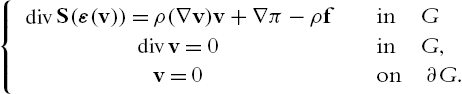
See for instance [23]. In physical terms this means that the fluid reached a steady state – a situation of balance. The unknown quantities are the velocity field v:G→Rd![]() and the pressure π:G→R
and the pressure π:G→R![]() . The function f:G→Rd
. The function f:G→Rd![]() represents a system of volume forces, while S:G→Rd×dsym
represents a system of volume forces, while S:G→Rd×dsym![]() is the viscous stress tensor and ρ>0
is the viscous stress tensor and ρ>0![]() is the density of the fluid. In order to describe a specific fluid one needs a constitutive law relating the viscous stress tensor S to the symmetric gradient ε(v):=12(∇v+∇vT)
is the density of the fluid. In order to describe a specific fluid one needs a constitutive law relating the viscous stress tensor S to the symmetric gradient ε(v):=12(∇v+∇vT)![]() of the velocity v. In the simplest case this relation is linear, i.e.,
of the velocity v. In the simplest case this relation is linear, i.e.,
S=S(ε(v))=2νε(v),
where ν>0![]() is the viscosity of the fluid. In this case we have divS=νΔv
is the viscosity of the fluid. In this case we have divS=νΔv![]() and (1.4.40) are the stationary Navier–Stokes equations (for a recent approach see [85,86]). The existence of a weak solution (where derivatives are to be understood in a distributional sense) can be established by arguments which are nowadays standard. In the case of the constitutive relation (1.4.41) the system (1.4.40) can be analysed like a linear system – the arguments used to handle the perturbation caused by (∇v)v
and (1.4.40) are the stationary Navier–Stokes equations (for a recent approach see [85,86]). The existence of a weak solution (where derivatives are to be understood in a distributional sense) can be established by arguments which are nowadays standard. In the case of the constitutive relation (1.4.41) the system (1.4.40) can be analysed like a linear system – the arguments used to handle the perturbation caused by (∇v)v![]() are of a technical nature (note that this is quite different from the parabolic situation), and standard techniques lead to smooth solutions (see for instance [86]).
are of a technical nature (note that this is quite different from the parabolic situation), and standard techniques lead to smooth solutions (see for instance [86]).
Only fluids with simple molecular structure e.g. water, oil and certain gases satisfy a linear relation such as (1.4.41). Those which do not are called non-Newtonian fluids (see [13]). A special class among these are generalized Newtonian fluids. Here, the viscosity is assumed to be a function of the shear rate |ε(v)|![]() and the constitutive relation is
and the constitutive relation is
S(ε(v))=ν(|ε(v)|)ε(v).
An external force can produce two different reactions:
• The fluid becomes thicker (for example batter): the viscosity of a shear thickening fluid is an increasing function of the shear rate.
• The fluid becomes thinner (for example ketchup): the viscosity of a shear thinning fluid is a decreasing function of the shear rate.
The power law model for non-Newtonian/generalized Newtonian fluids
S(ε(v))=ν0(1+|ε(v)|)p−2ε(v)
is very popular among rheologists. Here ν0>0![]() and p∈(1,∞)
and p∈(1,∞)![]() is specified by physical experiments. An extensive list of specific p-values for different fluids can be found in [23]. It becomes clear that many interesting p-values lie in the interval [32,2]
is specified by physical experiments. An extensive list of specific p-values for different fluids can be found in [23]. It becomes clear that many interesting p-values lie in the interval [32,2]![]() . In the following we give a historical overview concerning the theory of weak solutions to (1.4.40) and sketch the proofs, cf. [29].
. In the following we give a historical overview concerning the theory of weak solutions to (1.4.40) and sketch the proofs, cf. [29].
Monotone operator theory (1969).
The mathematical discussion of power law models started in the late sixties with the work of Lions and Ladyshenskaya (see [106–108] and [109]). Due to the appearance of the convective term div(v⊗v)![]() the equations for power law fluids (the constitutive law is given by (1.4.43)) depend significantly on the value of p. In the stationary case, the existence of a weak solution to (1.4.44), (1.4.43) can be shown by monotone operator theory for p⩾3dd+2
the equations for power law fluids (the constitutive law is given by (1.4.43)) depend significantly on the value of p. In the stationary case, the existence of a weak solution to (1.4.44), (1.4.43) can be shown by monotone operator theory for p⩾3dd+2![]() . To be precise, there is a function v∈W1,p0,div(G)
. To be precise, there is a function v∈W1,p0,div(G)![]() such that
such that
∫GS(ε(v)):ε(φ)dx=−ρ∫G(∇v)v⋅φdx+ρ∫Gf⋅φdx

for all φ∈C∞0,div(G)![]() . Note that this formulation has the advantage that the pressure does not appear but can easily be recovered later by De Rahm theory (this was first used in [109]). For the recovery of the pressure see Theorem 2.2.10. Also note that the divergence-free constraint and homogeneous boundary conditions are incorporated in the definition of the space W1,p0,div(G)
. Note that this formulation has the advantage that the pressure does not appear but can easily be recovered later by De Rahm theory (this was first used in [109]). For the recovery of the pressure see Theorem 2.2.10. Also note that the divergence-free constraint and homogeneous boundary conditions are incorporated in the definition of the space W1,p0,div(G)![]() . The condition
. The condition
p>3dd+2
ensures that the solution itself is a test-function and the convective term is a compact perturbation. We begin with the approach based on monotone operator theory (see [109]). It does not yet contain truncations, but it is the basis of the existence theory and everything is build upon it. Let us assume that (1.4.45) holds and that we have a sequence of approximate solutions, i.e. (vn)⊂W1,p0,div(G)![]() solving (1.4.44). We want to pass to the limit. By (1.4.45), Sobolev's embedding Theorem and smooth approximation, (1.4.44) holds also for all φ∈W1,p0,div(G)
solving (1.4.44). We want to pass to the limit. By (1.4.45), Sobolev's embedding Theorem and smooth approximation, (1.4.44) holds also for all φ∈W1,p0,div(G)![]() . So vn
. So vn![]() is an admissible test-function. Since ∫G(∇vn)vn⋅vndx=0
is an admissible test-function. Since ∫G(∇vn)vn⋅vndx=0![]() we obtain a uniform a priori estimate in W1,p(G)
we obtain a uniform a priori estimate in W1,p(G)![]() and (after choosing an appropriate subsequence)
and (after choosing an appropriate subsequence)
vn⇀vinW1,p0,div(G).
Note that we also used the coercivity from (1.4.43) and Korn's inequality. Using (1.4.43) again yields
S(ε(vn))⇀˜SinLp′(G).
The nonlinearity in the convective term (∇vn)vn![]() can be overcome by compactness arguments. Kondrachov's Theorem and (1.4.45) imply
can be overcome by compactness arguments. Kondrachov's Theorem and (1.4.45) imply
vn→vinL2p′(G)
and so
(∇vn)vn⇀(∇v)vinL2pp+1(G).
Using (1.4.46)–(1.4.49) we can pass to the limit in the equation and obtain
∫G˜S:ε(φ)dx=−∫G(∇v)v⋅φdx+∫Gf⋅φdx

for all φ∈W1,p0,div(G)![]() . It remains to be shown
. It remains to be shown
˜S=S(ε(v)).
As S is nonlinear the weak convergence in (1.4.46) is not enough for this limit procedure. We have to apply methods from monotone operator theory. Let us consider the integral
∫G(S(ε(vn))−S(ε(v))):(ε(vn)−ε(v))dx=∫GS(ε(vn)):(ε(vn)−ε(v))dx−∫GS(ε(v)):(ε(vn)−ε(v))dx.

The second term on the right-hand-side vanishes for n→∞![]() as a consequence of (1.4.46) and S(ε(v))∈Lp′(G)
as a consequence of (1.4.46) and S(ε(v))∈Lp′(G)![]() . For the first term one we use the equation for vn
. For the first term one we use the equation for vn![]() and obtain
and obtain
∫GS(ε(vn)):(ε(vn)−ε(v))dx=−∫G(∇vn)vn⋅(vn−v)dx+∫Gf⋅(vn−v)dx⟶0,n→∞.

This is a consequence of (1.4.46) and (1.4.49). Plugging all together we have shown
∫G(S(ε(vn))−S(ε(v))):(ε(vn)−ε(v))dx⟶0,n→∞.

The strict monotonicity of S implies ε(vn)→ε(v)![]() a.e. and hence (1.4.51).
a.e. and hence (1.4.51).
L∞
![]() -truncation (1997).
-truncation (1997).
Examining the three-dimensional situation we see that the bound p>95![]() is very restrictive since many interesting liquids lie beyond it. For example polyethylene oxide (polyethylene is the most common plastic) has lower flow behaviour indices: the experiments presented in [23] (table 4.1-2, p. 175) suggest values between 1.53 and 1.6 depending on the temperature. The first attempt to lower the bound for p was an approach via L∞
is very restrictive since many interesting liquids lie beyond it. For example polyethylene oxide (polyethylene is the most common plastic) has lower flow behaviour indices: the experiments presented in [23] (table 4.1-2, p. 175) suggest values between 1.53 and 1.6 depending on the temperature. The first attempt to lower the bound for p was an approach via L∞![]() -truncation by Frehse, Málek and Steinhauer (see [78], see also [129]). The term
-truncation by Frehse, Málek and Steinhauer (see [78], see also [129]). The term
∫G(∇v)v⋅φdx

is defined for all φ∈L∞(G)![]() if
if
p>2dd+1.
Instead of testing the equation by v (which is not permitted) they used the function vL∈L∞(G)![]() , L≫1
, L≫1![]() , whose L∞
, whose L∞![]() -norm is bounded by L and which equals v on a large set.
-norm is bounded by L and which equals v on a large set.
In order to give an overview of this method we assume that (1.4.52) holds and that we have a sequence of approximated solutions to (1.4.44) with uniform a priori estimates in W1,p0,div(G)![]() . Note that test-functions have to be bounded as (∇v)v
. Note that test-functions have to be bounded as (∇v)v![]() is only an integrable function. We will demonstrate how to obtain a weak solution combining ideas of [78] and [140].
is only an integrable function. We will demonstrate how to obtain a weak solution combining ideas of [78] and [140].
Again we have (1.4.46) and (1.4.47) but instead of (1.4.48) and (1.4.49) only the following hold
vn→vinLp′(G),
(∇vn)vn⇀(∇v)vinLσ(G),
where σ:=pdp(d+1)−2d∈(1,∞)![]() , cf. (1.4.52). We still obtain (1.4.50) for all φ∈W1,p0,div∩L∞(G)
, cf. (1.4.52). We still obtain (1.4.50) for all φ∈W1,p0,div∩L∞(G)![]() and the goal is to show (1.4.51). We are faced with the problem that the solution is not an admissible test-function any more. So an approach via monotone operator theory as described before will fail. Instead of testing with un:=vn−v
and the goal is to show (1.4.51). We are faced with the problem that the solution is not an admissible test-function any more. So an approach via monotone operator theory as described before will fail. Instead of testing with un:=vn−v![]() we use a truncated function. As functions from the class W1,p0,div∩L∞(G)
we use a truncated function. As functions from the class W1,p0,div∩L∞(G)![]() are admissible we cut values of un
are admissible we cut values of un![]() which are too large and obtain a bounded function. For L∈N
which are too large and obtain a bounded function. For L∈N![]() we define
we define
ΨL:=L∑ℓ=1ψ2−ℓ,ψδ(s):=ψ(δs),

where ψ∈C∞0([0,2])![]() , 0⩽ψ⩽1
, 0⩽ψ⩽1![]() , ψ≡1
, ψ≡1![]() on [0,1]
on [0,1]![]() and 0⩽−ψ′⩽2
and 0⩽−ψ′⩽2![]() . Now we use the test-function un,L:=ΨL(|un|)un
. Now we use the test-function un,L:=ΨL(|un|)un![]() and neglect for a moment the fact that it is not divergence-free. For fixed L the function un,L
and neglect for a moment the fact that it is not divergence-free. For fixed L the function un,L![]() is essentially bounded (in terms of L) and we obtain for n→∞
is essentially bounded (in terms of L) and we obtain for n→∞![]()
un,L→0inLq(G)for allq<∞.
Now we test with un,L![]() which implies (using (1.4.54) and (1.4.55) for the integral ∫G(∇vn)vn⋅un,Ldx
which implies (using (1.4.54) and (1.4.55) for the integral ∫G(∇vn)vn⋅un,Ldx![]() )
)
limsupn∫GΨL(|un|)(S(ε(vn))−S(ε(v))):ε(un)dx⩽limsupn∫GΨL(|un|)(S(ε(vn))−S(ε(v))):∇ΨL(|un|)⊗undx.

Now one needs that
∇ΨL(|un|)⊗un∈Lp(G)
uniformly in L and n which follows from the definition of ΨL![]() . This allows us to show that the left-hand-side of (1.4.56) is bounded in L and hence there is a subsequence (in fact one has to take a diagonal sequence) such that for n→∞
. This allows us to show that the left-hand-side of (1.4.56) is bounded in L and hence there is a subsequence (in fact one has to take a diagonal sequence) such that for n→∞![]()
σℓ,n:=∫G(S(ε(vn))−˜S)):ψ2−ℓ(|un|)ε(un)dx⟶σℓ,∀ℓ∈N0.

One can show easily that σℓ![]() is increasing in ℓ and so σ0=0
is increasing in ℓ and so σ0=0![]() , i.e.,
, i.e.,
∫G(S(ε(vn))−S(ε(v))):ψ1(|un|)ε(un)dx⟶0,n→0.

As ψ1(t)=1![]() for t⩽1
for t⩽1![]() and un→0
and un→0![]() in L2(G)
in L2(G)![]() this yields
this yields
∫G((S(ε(vn))−S(ε(v))):ε(un))Θdx⟶0,n→0,

for all Θ<1![]() . Due to the monotonicity of S we deduce (1.4.51).
. Due to the monotonicity of S we deduce (1.4.51).
As divun,L≠0![]() we have to correct the divergence by means of the Bogovskiĭ-operator. It is solution operator to the divergence equation with respect to zero boundary conditions. See Section 2.1. Additional terms appear which can be handled similarly.
we have to correct the divergence by means of the Bogovskiĭ-operator. It is solution operator to the divergence equation with respect to zero boundary conditions. See Section 2.1. Additional terms appear which can be handled similarly.
Remark 1.4.5
In [78] the limit case p=2dd+1![]() is also included based on the fact that (∇v)v
is also included based on the fact that (∇v)v![]() has div−curl
has div−curl![]() structure and hence belongs to the Hardy space H1(Rd)
structure and hence belongs to the Hardy space H1(Rd)![]() .
.
Lipschitz truncation (2003).
Although we can now cover a wide range of power law fluids there remain several with lower values of p. The experiments presented in [23] (table 4.1-2, p. 175) suggest values for 2% hydroxyethylcellulose (hydroxyethylcellulose is a gelling and thickening agent derived from cellulose, used in cosmetics, cleaning solutions, and other household products) between 1.19 and 1.25 depending on the temperature.
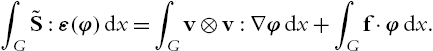
Since divv=0![]() we can rewrite
we can rewrite
∫G(∇v)v⋅φdx=−∫Gv⊗v:ε(φ)dx,

so that appropriate test-functions have to be Lipschitz continuous provided v⊗v∈L1(G)![]() . This condition is satisfied for p⩾2dd+2
. This condition is satisfied for p⩾2dd+2![]() by Sobolev's embedding. Otherwise one cannot define the convective term (at least in the stationary case). This bound therefore seems to be optimal.
by Sobolev's embedding. Otherwise one cannot define the convective term (at least in the stationary case). This bound therefore seems to be optimal.
In the case
p>2dd+2
the existence of a weak solution to (1.4.44), (1.4.43) was first established in [79]. This is the first paper where the Lipschitz truncation was used in the context of fluid mechanics. Here one approximates the function v by a Lipschitz continuous function vλ![]() with ‖∇vλ‖∞⩽cλ
with ‖∇vλ‖∞⩽cλ![]() instead of a bounded function as in the approach via L∞
instead of a bounded function as in the approach via L∞![]() -truncation.
-truncation.
Assume that (1.4.59) holds and that we have a sequence of solutions (vn)⊂W1,p0,div(G)![]() to
to
∫GS(ε(vn)):ε(φ)dx=∫Gvn⊗vn:∇φdx+∫Gf⋅φdx

for all φ∈W1,∞0,div(G)![]() which is uniformly bounded. Again we have (1.4.46) and (1.4.47) and by Kondrachov's Theorem and (1.4.59)
which is uniformly bounded. Again we have (1.4.46) and (1.4.47) and by Kondrachov's Theorem and (1.4.59)
vn→vinL2σ(G),vn⊗vn⇀v⊗vinLσ(G),
where σ∈(1,12pdd−p)![]() , cf. (1.4.59). So we can pass to the limit in (1.4.60) and obtain
, cf. (1.4.59). So we can pass to the limit in (1.4.60) and obtain
∫G˜S:ε(φ)dx=∫Gv⊗v:∇φdx+∫Gf⋅φdx.
In order to show ˜S=S(ε(v))![]() it is enough to have (1.4.58). Introduce the Lipschitz truncation un,λ
it is enough to have (1.4.58). Introduce the Lipschitz truncation un,λ![]() of un:=vn−v
of un:=vn−v![]() , cf. Section 1.3. Then (1.4.58) follows from
, cf. Section 1.3. Then (1.4.58) follows from
∫G(S(ε(vn))−S(ε(v))):ε(un,λ)dx⟶0,n→0,

and (1.3.31). As a consequence of ‖∇un,λ‖∞⩽cλ![]() the Lipschitz truncation features much better convergence properties than the original function. In particular, we have
the Lipschitz truncation features much better convergence properties than the original function. In particular, we have
un,λ→0inL∞(G),∇un,λ⇀⁎0inL∞(G),
recall (1.3.29) and (1.3.30). Taking this into account, (1.4.63) follows from (1.4.60) and (1.4.61).
We again neglected the fact that divun,λ≠0![]() . There are two options for overcoming this. In [79] the authors introduce the pressure πn
. There are two options for overcoming this. In [79] the authors introduce the pressure πn![]() and decompose it with respect to the terms appearing in the equation. This requires some technical effort but all terms can be handled. An easier way is presented in [62] where the divergence is corrected using the Bogovskiĭ operator as indicated in the approach via L∞
and decompose it with respect to the terms appearing in the equation. This requires some technical effort but all terms can be handled. An easier way is presented in [62] where the divergence is corrected using the Bogovskiĭ operator as indicated in the approach via L∞![]() -truncation.
-truncation.