
Fluid mechanics & Orlicz spaces
Abstract
We extend some classical tools from fluid mechanics – Korn's inequality, the Bogovskiĭ operator and the pressure recovery – to the setting of Orlicz spaces. As a special case the known Lp![]() -theory is included as well as the case of Orlicz spaces generated by a nice Young function (i.e., under Δ2
-theory is included as well as the case of Orlicz spaces generated by a nice Young function (i.e., under Δ2![]() and ∇2
and ∇2![]() condition). In the general case there is some loss of integrability, for instance in the limit cases LlogL→L1
condition). In the general case there is some loss of integrability, for instance in the limit cases LlogL→L1![]() and L∞→Exp(L)
and L∞→Exp(L)![]() . The results are shown to be optimal in the sense of Orlicz spaces.
. The results are shown to be optimal in the sense of Orlicz spaces.
Keywords
Orlicz spaces; Divergence equation; Bogovskiĭ operator; Negative norm theorem; Pressure recovery; Korn's inequality
A crucial tool in the mathematical approach to the behaviour of Newtonian fluids is Korn's inequality: given a bounded open domain G⊂Rd![]() , d⩾2
, d⩾2![]() , with Lipschitz boundary ∂G we have
, with Lipschitz boundary ∂G we have
∫G|∇v|2dx⩽2∫G|ε(v)|2dx
for all v∈W1,20(G)![]() . For smooth functions with compact support (2.0.1) can be shown by integration by parts. The general case is treated by approximation. A first proof was given by Korn in [104]. We note that variants of Korn's inequality in L2
. For smooth functions with compact support (2.0.1) can be shown by integration by parts. The general case is treated by approximation. A first proof was given by Korn in [104]. We note that variants of Korn's inequality in L2![]() have been established by Courant and Hilbert [53], Friedrichs [84], Èidus [70] and Mihlin [114]. Many problems in the mathematical theory of generalized Newtonian fluids and mechanics of solids lead to the following question (compare for example the monographs of Málek, Nečas, Rokyta and Růžička [111], of Duvaut and Lions [66] and of Zeidler [143]): is it possible to bound a suitable energy depending on ∇v
have been established by Courant and Hilbert [53], Friedrichs [84], Èidus [70] and Mihlin [114]. Many problems in the mathematical theory of generalized Newtonian fluids and mechanics of solids lead to the following question (compare for example the monographs of Málek, Nečas, Rokyta and Růžička [111], of Duvaut and Lions [66] and of Zeidler [143]): is it possible to bound a suitable energy depending on ∇v![]() by the corresponding functional of ε(v)
by the corresponding functional of ε(v)![]() , that is
, that is
∫G|∇v|pdx⩽c(p,G)∫G|ε(v)|pdx

for functions v∈W1,p0(G)![]() ? As shown by Gobert [91,92], Nečas [119], Mosolov and Mjasnikov [116], Temam [138] and later by Fuchs [74] this is true for all 1<p<∞
? As shown by Gobert [91,92], Nečas [119], Mosolov and Mjasnikov [116], Temam [138] and later by Fuchs [74] this is true for all 1<p<∞![]() (we remark that the inequality fails in the case p=1
(we remark that the inequality fails in the case p=1![]() , see [120] and [52]).
, see [120] and [52]).
A first step in the generalization of (2.0.2) is mentioned in [4]: Acerbi and Mingione prove a variant for the Young function
A(t)=(1+t2)p−22t2.
More precisely, they show that
‖∇v‖LA(G)⩽c(φ,G)‖ε(v)‖LA(G)
for all functions v∈W1,A0(G)![]() . Although they only consider a special case they provide tools for much more general situations. Note that they only obtain inequalities in the Luxembourg-norm which is not appropriate in many situations (for example in regularity theory, see [35]). A general theorem is proved in [64], namely that
. Although they only consider a special case they provide tools for much more general situations. Note that they only obtain inequalities in the Luxembourg-norm which is not appropriate in many situations (for example in regularity theory, see [35]). A general theorem is proved in [64], namely that
∫GA(|∇v−(∇v)G|)dx⩽c(A,G)∫GA(|ε(v)−(ε(v))G|)dx

for all v∈W1,A(G)![]() , where A is a Young function satisfying the Δ2
, where A is a Young function satisfying the Δ2![]() - and ∇2
- and ∇2![]() -condition. Furthermore, Fuchs [75] obtains (2.0.4) for functions with zero traces and the same class of Young functions by a different approach. It is shown in [32] that the Δ2
-condition. Furthermore, Fuchs [75] obtains (2.0.4) for functions with zero traces and the same class of Young functions by a different approach. It is shown in [32] that the Δ2![]() - and ∇2
- and ∇2![]() -condition are also necessary for the inequality (2.0.4). We remark that the constitutive law
-condition are also necessary for the inequality (2.0.4). We remark that the constitutive law
S=A′(|ε(v)|)|ε(v)|ε(v)

for a Young function A is a quite general model to describe the motion of generalized Newtonian fluids (see, i.e., [35], [25] and [59]).
In order to characterize the behaviour of Prandtl–Eyring fluids (see Chapter 4) Eyring [69] suggested the constitutive law
S=DW(ε(u)),W(ε)=h(|ε|)=|ε|log(1+|ε|).
This leads in a natural way to the question about Korn's inequality in the space Lh(G)![]() . Since we have
. Since we have
˜h(t)≈t(exp(t)−1),
the ∇2![]() -condition fails in this case, hence the results mentioned above do not apply. So the following question remains: given some integrability of the symmetric gradient – in the sense of Orlicz spaces – what is the best integrability for the full gradient we can expect?
-condition fails in this case, hence the results mentioned above do not apply. So the following question remains: given some integrability of the symmetric gradient – in the sense of Orlicz spaces – what is the best integrability for the full gradient we can expect?
A second fundamental question in fluid mechanics is the recovery of the pressure. It is common (and very useful) to study pressure-free formulations of (generalized) Navier–Stokes equations. So one starts by finding a velocity field which solves the corresponding system in the sense of distributions on divergence-free test-functions. Afterwards there is the question about the existence of the pressure function in order to have a weak solution in the sense of distributions.
Let us be a bit more precise and consider the equation
∫GH:∇φdx=0for allφ∈C∞0,div(G),

where H is an integrable function (in case of a stationary generalized Navier–Stokes equation we have H=S(ε(v))+∇Δ−1f−v⊗v![]() ). Secondly, the pressure π is reconstructed in the sense that
). Secondly, the pressure π is reconstructed in the sense that
∫GH:∇φdx=∫Ωπdivφdxfor allφ∈C∞0(G).

The existence of a pressure in the sense of distributions is a consequence of the classical theorem by De Rahm (see [131] for an appropriate version). It is also well-known that – if 1<p<∞![]() – then H∈Lp(G)
– then H∈Lp(G)![]() implies π∈Lp(G)
implies π∈Lp(G)![]() . This result breaks down in the limit cases. Again motivated by the Prandtl–Eyring model the following question remains: given a function H solving (2.0.6) – located in some Orlicz space – what is the optimal integrability of the pressure in (2.0.7)?
. This result breaks down in the limit cases. Again motivated by the Prandtl–Eyring model the following question remains: given a function H solving (2.0.6) – located in some Orlicz space – what is the optimal integrability of the pressure in (2.0.7)?
In classical Lp![]() -spaces, both questions raised above can be answered by Nečas' negative norm theorem [119]. The negative Sobolev norm of the distributional gradient of a function u∈L1(G)
-spaces, both questions raised above can be answered by Nečas' negative norm theorem [119]. The negative Sobolev norm of the distributional gradient of a function u∈L1(G)![]() can be defined as
can be defined as
‖∇u‖W−1,p(G)=supφ∈C∞0(G)∫Gudivφdx‖∇φ‖Lp′(G)dx,

where 1⩽p⩽∞![]() . In (2.0.8), and in similar occurrences throughout this chapter, we tacitly assume that the supremum is extended over all functions v which do not vanish identically. We remark that the quantity on the right-hand side of (2.0.8) agrees with the norm of ∇u, when regarded as an element of the dual of W1,p′0(G)
. In (2.0.8), and in similar occurrences throughout this chapter, we tacitly assume that the supremum is extended over all functions v which do not vanish identically. We remark that the quantity on the right-hand side of (2.0.8) agrees with the norm of ∇u, when regarded as an element of the dual of W1,p′0(G)![]() . Nečas showed that, if G is regular enough – a bounded Lipschitz domain, say – and 1<p<∞
. Nečas showed that, if G is regular enough – a bounded Lipschitz domain, say – and 1<p<∞![]() , then the Lp(G)
, then the Lp(G)![]() norm of a function is equivalent to the W−1,p(G)
norm of a function is equivalent to the W−1,p(G)![]() norm of its gradient. Namely, there exist positive constants C1=C1(G,p)
norm of its gradient. Namely, there exist positive constants C1=C1(G,p)![]() and C2=C2(d)
and C2=C2(d)![]() , such that
, such that
C1‖u−uG‖Lp(G)⩽‖∇u‖W−1,p(G)⩽C2‖u−uG‖Lp(G)
for every u∈L1(G)![]() .
.
Using the formula
Δu=divV(u),Vij(u)=2εD(u)−(12−1d)(divu)I,
where εD=ε−1dtrεI![]() , the proof of Korn's inequality based on (2.0.9) is elementary. Moreover, a combination of De Rahm's Theorem and (2.0.9) shows that if H∈Lp(G)
, the proof of Korn's inequality based on (2.0.9) is elementary. Moreover, a combination of De Rahm's Theorem and (2.0.9) shows that if H∈Lp(G)![]() satisfies (2.0.6) then there is π∈Lp(G)
satisfies (2.0.6) then there is π∈Lp(G)![]() such that (2.0.7) holds.
such that (2.0.7) holds.
In order to understand how Korn's inequality and the pressure recovery work in Orlicz spaces, we have to understand Orlicz versions of (2.0.9). Let A be a Young function, and let G be a bounded domain in Rd![]() . We define the negative Orlicz–Sobolev norm associated with A of the distributional gradient of a function u∈L1(G)
. We define the negative Orlicz–Sobolev norm associated with A of the distributional gradient of a function u∈L1(G)![]() as
as
‖∇u‖W−1,A(G)=supφ∈C∞0(G,Rn)∫Gudivφdx‖∇φ‖L˜A(G).

The alternative notation W−1LA(G)![]() will also occasionally be employed to denote the negative Orlicz–Sobolev norm W−1,A(G)
will also occasionally be employed to denote the negative Orlicz–Sobolev norm W−1,A(G)![]() associated with the Orlicz space LA(G)
associated with the Orlicz space LA(G)![]() . As (2.0.9) is known to break down in the limit cases, an Orlicz-version with the same Young function on both sides cannot hold in general. In fact, our Orlicz–Sobolev space version of the negative norm theorem involves pairs of Young functions A and B which obey the following balance conditions:
. As (2.0.9) is known to break down in the limit cases, an Orlicz-version with the same Young function on both sides cannot hold in general. In fact, our Orlicz–Sobolev space version of the negative norm theorem involves pairs of Young functions A and B which obey the following balance conditions:
t∫t0B(s)s2ds⩽A(ct)fort⩾0,

and
t∫t0˜A(s)s2ds⩽˜B(ct)fort⩾0,

for some positive constant c. Note that the same conditions come into play in the study of singular integral operators in Orlicz spaces [47].
If either (2.0.11) or (2.0.12) holds, then A dominates B globally [48, Proposition 3.5]. In a sense, the assumptions (2.0.11) and (2.0.12) provide us with a quantitative information about how much weaker the norm ‖⋅‖LB(G)![]() is than ‖⋅‖LA(G)
is than ‖⋅‖LA(G)![]() . Under these assumptions a version of the negative norm theorem can be restored in Orlicz–Sobolev spaces.
. Under these assumptions a version of the negative norm theorem can be restored in Orlicz–Sobolev spaces.
Theorem 2.0.5
Let A and B be Young functions, fulfilling (2.0.11) and (2.0.12). Assume that G is a bounded domain with the cone property in Rd![]() , d⩾2
, d⩾2![]() . Then there exist constants C1=C1(G,c)
. Then there exist constants C1=C1(G,c)![]() and C2=C2(d)
and C2=C2(d)![]() such that
such that
C1‖u−uG‖LB(G)⩽‖∇u‖W−1,A(G)⩽C2‖u−uG‖LA(G)
for every u∈L1(G)![]() . Here, c denotes the constant appearing in (2.0.11) and (2.0.12).
. Here, c denotes the constant appearing in (2.0.11) and (2.0.12).
Remark 2.0.6
Inequality (2.0.13) continues to hold even if conditions (2.0.11) and (2.0.12) are just fulfilled for t⩾t0![]() for some t0>0
for some t0>0![]() , but with constants C1
, but with constants C1![]() and C2
and C2![]() depending also on A, B, t0
depending also on A, B, t0![]() and |G|
and |G|![]() . Indeed, the Young functions A and B can be replaced, if necessary, with Young functions which are equivalent near infinity and fulfil (2.0.11) and (2.0.12) for every t>0
. Indeed, the Young functions A and B can be replaced, if necessary, with Young functions which are equivalent near infinity and fulfil (2.0.11) and (2.0.12) for every t>0![]() . Due to (1.2.11), such replacement leaves the quantities ‖⋅‖LA(G)
. Due to (1.2.11), such replacement leaves the quantities ‖⋅‖LA(G)![]() , ‖⋅‖LB(G)
, ‖⋅‖LB(G)![]() and ‖∇⋅‖W−1,A(G)
and ‖∇⋅‖W−1,A(G)![]() unchanged, up to multiplicative constants depending on A, B, t0
unchanged, up to multiplicative constants depending on A, B, t0![]() and |G|
and |G|![]() .
.
The situations when (2.0.11), or (2.0.12), holds with B=A![]() can be precisely characterized. Membership of A to Δ2
can be precisely characterized. Membership of A to Δ2![]() is a necessary and sufficient condition for (2.0.12) to hold with B=A
is a necessary and sufficient condition for (2.0.12) to hold with B=A![]() [103, Theorem 1.2.1]. Therefore, under this condition, assumption (2.0.12) can be dropped in Theorem 2.0.5. On the other hand, A∈∇2
[103, Theorem 1.2.1]. Therefore, under this condition, assumption (2.0.12) can be dropped in Theorem 2.0.5. On the other hand, A∈∇2![]() if and only if ˜A∈Δ2
if and only if ˜A∈Δ2![]() . Hence membership of A to ∇2
. Hence membership of A to ∇2![]() is a necessary and sufficient condition for (2.0.11) to hold with B=A
is a necessary and sufficient condition for (2.0.11) to hold with B=A![]() . Thus, under this condition, assumption (2.0.11) can be dropped in Theorem 2.0.5. Particularly, if A∈Δ2∩∇2
. Thus, under this condition, assumption (2.0.11) can be dropped in Theorem 2.0.5. Particularly, if A∈Δ2∩∇2![]() , then both conditions (2.0.11) and (2.0.12) are fulfilled with B=A
, then both conditions (2.0.11) and (2.0.12) are fulfilled with B=A![]() . Hence, we have the following corollary which also follows from the results of [64].
. Hence, we have the following corollary which also follows from the results of [64].
Corollary 2.0.1
A typical situation where condition (2.0.11) does not hold with B=A![]() is when A grows linearly, or “almost linearly”, near infinity. In this case, A∉∇2
is when A grows linearly, or “almost linearly”, near infinity. In this case, A∉∇2![]() . In fact, as already mentioned, the standard negative norm theorem expressed by (2.0.9) breaks down in the borderline case p=1
. In fact, as already mentioned, the standard negative norm theorem expressed by (2.0.9) breaks down in the borderline case p=1![]() . On the other hand, condition (2.0.12) fails, with B=A
. On the other hand, condition (2.0.12) fails, with B=A![]() , if, for example, A has a very fast – faster than any power – growth. In this case, A∉Δ2
, if, for example, A has a very fast – faster than any power – growth. In this case, A∉Δ2![]() . Loosely speaking, the norm ‖⋅‖LA(G)
. Loosely speaking, the norm ‖⋅‖LA(G)![]() is now “close” to ‖⋅‖L∞(G)
is now “close” to ‖⋅‖L∞(G)![]() , and, as a matter of fact, equation (2.0.9) is not true with p=∞
, and, as a matter of fact, equation (2.0.9) is not true with p=∞![]() .
.
These, however, are not the only situations when (2.0.11), or (2.0.12), fail with B=A![]() . For instance, there are functions A which neither satisfy the Δ2
. For instance, there are functions A which neither satisfy the Δ2![]() condition, nor the ∇2
condition, nor the ∇2![]() condition. Therefore, neither (2.0.12) nor (2.0.11) can hold with B=A
condition. Therefore, neither (2.0.12) nor (2.0.11) can hold with B=A![]() . In those cases A(t)
. In those cases A(t)![]() “oscillates” between two different powers tp
“oscillates” between two different powers tp![]() and tq
and tq![]() , with 1<p<q<∞
, with 1<p<q<∞![]() . Functions of this kind are referred to as (p,q)
. Functions of this kind are referred to as (p,q)![]() -growth in the literature. Partial differential equations, and associated variational problems, whose nonlinearity is governed by this growth, have been extensively studied. In the framework of non-Newtonian fluids, they have been analysed in [22].
-growth in the literature. Partial differential equations, and associated variational problems, whose nonlinearity is governed by this growth, have been extensively studied. In the framework of non-Newtonian fluids, they have been analysed in [22].
All the circumstances described above can be handled via Theorem 2.0.5. A few examples involving customary families of Young functions are presented hereafter.
Example 1
Assume that A(t)![]() is a Young function equivalent to tplogα(1+t)
is a Young function equivalent to tplogα(1+t)![]() near infinity, where either p>1
near infinity, where either p>1![]() and α∈R
and α∈R![]() , or p=1
, or p=1![]() and α⩾1
and α⩾1![]() . Hence, if |G|<∞
. Hence, if |G|<∞![]() , then
, then
LA(G)=LplogαL(G).
Assume that G is a bounded domain with the cone property in Rd![]() . If p>1
. If p>1![]() , then A∈Δ2∩∇2
, then A∈Δ2∩∇2![]() , and hence Corollary 2.0.1 tells us that
, and hence Corollary 2.0.1 tells us that
C1‖u−uG‖LplogαL(G)⩽‖∇u‖W−1LplogαL(G)⩽C2‖u−uG‖LplogαL(G)
for every u∈L1(G)![]() . However, if p=1
. However, if p=1![]() , then A∈Δ2
, then A∈Δ2![]() , but A∉∇2
, but A∉∇2![]() . An application of Theorem 2.0.5 now implies
. An application of Theorem 2.0.5 now implies
C1‖u−uG‖Llogα−1L(G)⩽‖∇u‖W−1LlogαL(G)⩽C2‖u−uG‖LlogαL(G)
for every u∈L1(G)![]() . In particular,
. In particular,
C1‖u−uG‖L1(G)⩽‖∇u‖W−1LlogL(G)⩽C2‖u−uG‖LlogL(G)
for every u∈L1(G)![]() .
.
Example 2
Let β>0![]() , and let A(t)
, and let A(t)![]() be a Young function equivalent to exp(tβ)
be a Young function equivalent to exp(tβ)![]() near infinity. Then
near infinity. Then
LA(G)=expLβ(G)
if |G|<∞![]() . One has that A∈∇2
. One has that A∈∇2![]() , but A∉Δ2
, but A∉Δ2![]() . Theorem 2.0.5 ensures that, if G is a bounded domain with the cone property in Rd
. Theorem 2.0.5 ensures that, if G is a bounded domain with the cone property in Rd![]() , then
, then
C1‖u−uG‖expLββ+1(G)⩽‖∇u‖W−1expLβ(G)⩽C2‖u−uG‖expLβ(G)
for every u∈L1(G)![]() . Moreover,
. Moreover,
C1‖u−uG‖expL(G)⩽‖∇u‖W−1L∞(G)⩽C2‖u−uG‖L∞(G)
for every u∈L1(G)![]() .
.
Our approach is based on a study of the Bogovskiĭ operator [24] in Orlicz spaces in Theorem 2.1.7 which is already interesting itself. The Bogovskiĭ operator is a solution operator to the divergence equation with respect to zero boundary conditions. The continuity of the Bogovskiĭ operator implies the negative norm Theorem from which we can deduce both, the pressure recovery and Korn's inequality.
In Theorem 2.2.10 we give the precise statement of the pressure recovery in Orlicz spaces. In fact, H∈LA(G)![]() implies π∈LB(G)
implies π∈LB(G)![]() where A and B are linked through (2.0.11) and (2.0.12). Moreover, the following inequality holds
where A and B are linked through (2.0.11) and (2.0.12). Moreover, the following inequality holds
∫GB(|π|)dx⩽∫GA(C|H−HG|)dx.

Theorem 2.3.12 contains a version of Korn's inequality in general Orlicz spaces which says
∫GB(|∇u−(∇u)G|)dx⩽∫GA(C|ε(u)−(ε(u))G|)dx.

The final question which remains is the sharpness of the mentioned results. In Section 2.3 we are going to show that the balance conditions (2.0.11) and (2.0.12) are also necessary for a Korn's inequality. This implies that also the results about negative norms in Theorem 2.0.5 and the Bogovskiĭ operator in Theorem 2.1.6 are optimal.
2.1 Bogovskiĭ operator
Our proof of Theorem 2.0.5 relies upon an analysis of the divergence equation
{divu=finG,u=0on∂G,

in Orlicz spaces which we analyse in the following. Subsequently, we set
C∞0,⊥(G)={u∈C∞0(G):uG=0},LA⊥(G)={u∈LA(G):uG=0},

where uG=⨍Gudx![]() denotes the mean value of the function u.
denotes the mean value of the function u.
Theorem 2.1.6
Assume that G is a bounded domain with the cone property in Rd![]() , d⩾2
, d⩾2![]() . Let A and B be Young functions fulfilling (2.0.11 and (2.0.12). Then there exists a bounded linear operator
. Let A and B be Young functions fulfilling (2.0.11 and (2.0.12). Then there exists a bounded linear operator
BogG:LA⊥(G)→W1,B0(G)
such that
BogG:C∞0,⊥(G)→C∞0(G)
and
div(BogGf)=fin G
for every f∈LA⊥(G)![]() . In particular, there exists a constant C=C(G,c)
. In particular, there exists a constant C=C(G,c)![]() such that
such that
‖∇(BogGf)‖LB(G)⩽C‖f‖LA(G)
and
∫GB(|∇(BogGf)|)dx⩽∫GA(C|f|)dx

for every f∈LA⊥(G)![]() . Here, c denotes the constant appearing in (2.0.11) and (2.0.12).
. Here, c denotes the constant appearing in (2.0.11) and (2.0.12).
Although it will not be used for our main purposes, we state in Theorem 2.1.7 below a result parallel to Theorem 2.1.6, dealing with a version of problem (2.1.20) in the case when the right-hand side of the equation is in divergence form. Namely,
{divu=divginG,u=0on∂G,
where g:G→Rd![]() is a given function satisfying the compatibility condition (in a weak sense) that its normal component on ∂G vanishes. As a precise formulation of this condition we consider the space HA(G)
is a given function satisfying the compatibility condition (in a weak sense) that its normal component on ∂G vanishes. As a precise formulation of this condition we consider the space HA(G)![]() of those vector-valued functions u:G→Rn
of those vector-valued functions u:G→Rn![]() for which the norm
for which the norm
‖u‖HA(G)=‖u‖LA(G,Rn)+‖divu‖LA(G)
is finite. We denote by HA0(G)![]() its subspace of those functions u∈HA(G)
its subspace of those functions u∈HA(G)![]() whose normal component on ∂G vanishes, in the sense that
whose normal component on ∂G vanishes, in the sense that
∫Gφdivudx=−∫Gu⋅∇φdx
for every φ∈C∞(‾G)![]() . It is easy to see that both HA(G)
. It is easy to see that both HA(G)![]() and HA0(G)
and HA0(G)![]() are Banach spaces.
are Banach spaces.
Theorem 2.1.7
Assume that G is a bounded Lipschitz domain in Rd![]() , d⩾2
, d⩾2![]() . Let A and B be Young functions fulfilling (2.0.11) and (2.0.12). Then there exists a bounded linear operator
. Let A and B be Young functions fulfilling (2.0.11) and (2.0.12). Then there exists a bounded linear operator
EG:HA0(G)→W1,B0(G)
such that
div(EGg)=divginG
for every g∈HA0(G)![]() . In particular, there exists a constant C=C(G,c)
. In particular, there exists a constant C=C(G,c)![]() such that
such that
‖∇(EGg)‖LB(G)⩽C‖divg‖LA(G)
and
‖EGg‖LB(G)⩽C‖g‖LA(G)
for every g∈HA0(G)![]() . Here, c denotes the constant appearing in (2.0.11) and (2.0.12).
. Here, c denotes the constant appearing in (2.0.11) and (2.0.12).
The proofs of Theorems 2.1.6 and 2.1.7 make use of a rearrangement estimate, which extends those of [18, Theorem 16.12] and [15], for a class of singular integral operators of the form
Tf(x)=limε→0+∫{y:|y−x|>ε}K(x,y)f(y)dyforx∈Rd,

for an integrable function f:Rd→R![]() . Here K(x,y)=N(x,x−y)
. Here K(x,y)=N(x,x−y)![]() , where the kernel N:Rd×Rd→R
, where the kernel N:Rd×Rd→R![]() fulfills the following properties:
fulfills the following properties:
N(x,λz)=λ−dN(x,z)forx,z∈Rd;
∫Sd−1N(x,z)dHd−1(z)=0forx∈Rd;

For every σ∈[1,∞)![]() , there exists a constant C1
, there exists a constant C1![]() such that
such that
(∫Sd−1|N(x,z)|σdHd−1(y))1σ⩽C1(1+|x|)dforx∈Rd,

where Ss−1![]() denotes the unit sphere, centered at 0 in Rd
denotes the unit sphere, centered at 0 in Rd![]() , and Hs−1
, and Hs−1![]() stands for the (s−1)
stands for the (s−1)![]() -dimensional Hausdorff measure.
-dimensional Hausdorff measure.
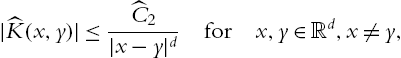
There exists a constant C2![]() such that
such that
|K(x,y)|⩽C2(1+|x|)d|x−y|sforx,y∈Rd,x≠y,

and, if 2|x−z|<|x−y|![]() , then
, then
|K(x,y)−K(z,y)|⩽C2(1+|y|)d|x−z||x−y|d+1,

|K(y,x)−K(y,z)|⩽C2(1+|y|)d|x−z||x−y|d+1.

Theorem 2.1.8
Let G be a bounded open set in Rd![]() , and let K be a kernel satisfying (2.1.34)–(2.1.39). If f∈L1(Rd)
, and let K be a kernel satisfying (2.1.34)–(2.1.39). If f∈L1(Rd)![]() and f=0
and f=0![]() in Rd∖G
in Rd∖G![]() , then the singular integral operator T given by (2.1.33) is well defined for a.e. x∈Rd
, then the singular integral operator T given by (2.1.33) is well defined for a.e. x∈Rd![]() , and there exists a constant C=C(C1,C2,d,diam(G))
, and there exists a constant C=C(C1,C2,d,diam(G))![]() for which
for which
(Tf)⁎(s)⩽C(1s∫s0f⁎(r)dr+∫|G|sf⁎(r)drr)fors∈(0,|G|).

As a consequence of Theorem 2.1.8, the boundedness of singular integral operators given by (2.1.33) between Orlicz spaces associated with Young functions A and B fulfilling (2.0.11) and (2.0.12) can be established.
Theorem 2.1.9
Let G, K and T be as in Theorem 2.1.8. Assume that A and B are Young functions satisfying (2.0.11) and (2.0.12). Then there exists a constant C=C(C1,C2,d,diam(G),c)![]() such that
such that
‖Tf‖LB(G)⩽C‖f‖LA(G),
and
∫GB(|Tf|)dx⩽∫GA(C|f|)dx

for every f∈LA(G)![]() . Here, c denotes the constant appearing in (7.0.1) and (5.3.12).
. Here, c denotes the constant appearing in (7.0.1) and (5.3.12).
Proof
According to Lemma 1.2.1, if A and B are Young functions satisfying (2.0.11), then there exists a constant C=C(c)![]() such that
such that
‖1s∫s0φ(r)dr‖LB(0,∞)⩽C‖φ‖LA(0,∞)

for every φ∈LA(0,∞)![]() . Moreover, if A and B fulfil (2.0.12), then there exists a constant C=C(c)
. Moreover, if A and B fulfil (2.0.12), then there exists a constant C=C(c)![]() such that
such that
‖∫∞sφ(r)drr‖LB(0,∞)⩽C‖φ‖LA(0,∞)

for every φ∈LA(0,∞)![]() . Combining (2.1.40), (2.1.43) and (2.1.44), and making use of property (1.2.12) implies inequality (2.1.41).
. Combining (2.1.40), (2.1.43) and (2.1.44), and making use of property (1.2.12) implies inequality (2.1.41).
As far as (2.1.42) is concerned, observe that, inequalities (2.0.11) and (2.0.12) continue to hold, with the same constant c, if A and B are replaced with kA and kB, where k is any positive constant. Thus, inequality (2.1.41) continues to hold, with the same constant C, after this replacement, whatever k is, namely
‖Tf‖LkB(G)⩽C‖f‖LkA(G)
for every f∈LA(G)![]() . Now, given any such f, choose k=1∫GA(|f|)dx
. Now, given any such f, choose k=1∫GA(|f|)dx![]() . The very definition of Luxemburg norm tells us that ‖f‖LkA(G)⩽1
. The very definition of Luxemburg norm tells us that ‖f‖LkA(G)⩽1![]() . Hence, by (2.1.45), ‖Tf‖LkB(G)⩽C
. Hence, by (2.1.45), ‖Tf‖LkB(G)⩽C![]() . The definition of Luxemburg norm again implies that ∫GkB(|Tf|C)dx⩽1
. The definition of Luxemburg norm again implies that ∫GkB(|Tf|C)dx⩽1![]() , namely (2.1.42). □
, namely (2.1.42). □
Proof of Theorem 2.1.8
Let R>0![]() be such that G⊂BR(0)
be such that G⊂BR(0)![]() , the ball centered at 0, with radius R. Fix a smooth function η:[0,∞)→[0,∞)
, the ball centered at 0, with radius R. Fix a smooth function η:[0,∞)→[0,∞)![]() for which η=1
for which η=1![]() in [0,3R]
in [0,3R]![]() and η=0
and η=0![]() in [4R,∞)
in [4R,∞)![]() . Define
. Define
ˆN(x,z)=η(|x|)N(x,z)forx,z∈Rd,ˆK(x,y)=ˆN(x,x−y)forx,y∈Rd.
By properties (2.1.34)–(2.1.39), one has that:
ˆN(x,λy)=λ−dˆN(x,z)forx,z∈Rd;
∫Sd−1ˆN(x,z)dHd−1(z)=0forx∈Rd;

for every σ∈[1,∞)![]() , there exists a constant ˆC1=ˆC1(C1,σ,R,d)
, there exists a constant ˆC1=ˆC1(C1,σ,R,d)![]() such that
such that
(∫Sd−1|ˆN(x,z)|σdHd−1(z))1σ⩽ˆC1forx∈Rd,

where C1![]() is the constant appearing in (2.1.36); there exists a constant ˆC2=ˆC2(C2,R,d)
is the constant appearing in (2.1.36); there exists a constant ˆC2=ˆC2(C2,R,d)![]() for which
for which
|ˆK(x,y)|⩽ˆC2|x−y|dforx,y∈Rd,x≠y,
and, if x∈Rd![]() , y∈G
, y∈G![]() and 2|x−z|<|x−y|
and 2|x−z|<|x−y|![]() , then
, then
|ˆK(x,y)−ˆK(z,y)|⩽ˆC2|x−z||x−y|d+1,

|ˆK(y,x)−ˆK(y,z)|⩽ˆC2|x−z||x−y|d+1,

where C2![]() is the constant appearing in (2.1.37)–(2.1.39). Define
is the constant appearing in (2.1.37)–(2.1.39). Define
ˆTεf(x)=∫{y:|y−x|>ε}ˆK(x,y)f(y)dy,ˆTSf(x)=supε>0|ˆTε(f)(x)|.

Inequality (2.1.40) will follow if we prove that
(ˆTSf)⁎(s)⩽C(1s∫s0f⁎(r)dr+∫|G|sf⁎(r)drr)fors∈(0,∞)

for some constant C=C(C1,C2,d,R)![]() , and for every f∈L1(Rd)
, and for every f∈L1(Rd)![]() for which f=0
for which f=0![]() in Rd∖BR(0)
in Rd∖BR(0)![]() . A proof of inequality (2.1.52) can be accomplished along the same lines as that of Theorem 1 of [15], which in turn relies upon similar techniques as in [51]. For completeness, we give the details of the proof hereafter.
. A proof of inequality (2.1.52) can be accomplished along the same lines as that of Theorem 1 of [15], which in turn relies upon similar techniques as in [51]. For completeness, we give the details of the proof hereafter.
The key step in the derivation of (2.1.52) consists in showing that, for every γ∈(0,1)![]() , there exists a constant C=C(C1,C2,γ,d,R)
, there exists a constant C=C(C1,C2,γ,d,R)![]() such that
such that
(ˆTSf)⁎(s)⩽C(Mf)⁎(γs)+(ˆTSf)⁎(2s)fors∈(0,∞)
for every f∈L1(Rd)![]() with f=0
with f=0![]() in Rd∖BR(0)
in Rd∖BR(0)![]() . Fix s>0
. Fix s>0![]() , and define
, and define
E={x∈Rd:ˆTSf(x)>(ˆTSf)⁎(2s)}.
Then, there exists an open set U⊃E![]() for which |U|⩽3s
for which |U|⩽3s![]() . By Whitney's covering theorem, there exist a family of disjoint cubes {Qk}
. By Whitney's covering theorem, there exist a family of disjoint cubes {Qk}![]() such that U=∪∞k=1Qk
such that U=∪∞k=1Qk![]() , ∑∞k=1|Qk|=|U|⩽3s
, ∑∞k=1|Qk|=|U|⩽3s![]() , and
, and
diam(Qk)⩽dist(Qk,Rd∖U)⩽4diam(Qk)fork∈N.
The operator ˆTS![]() is of weak type (1,1)
is of weak type (1,1)![]() , namely, there exists a constant C′
, namely, there exists a constant C′![]() such that
such that
|{x∈Rd:ˆTSf(x)>λ}|⩽C′λ‖f‖L1(Rd)
for f∈L1(Rd)![]() . The proof of (2.1.54) follows from classical arguments: By (2.1.51) we have for all r>0
. The proof of (2.1.54) follows from classical arguments: By (2.1.51) we have for all r>0![]() , y∈Rd
, y∈Rd![]() and all x∈Br(z)
and all x∈Br(z)![]() that
that
∫|y−x|⩾2r|ˆK(y,x)−ˆK(y,z)|dy⩽C.

So ˆK![]() satisfies condition (10) in [134, p. 33]. By [134, Cor. 1, p. 33] we obtain
satisfies condition (10) in [134, p. 33]. By [134, Cor. 1, p. 33] we obtain
|{x∈Rd:ˆTεf(x)>λ}|⩽Cλ‖f‖L1(Rd),
where C does not depend on ε. Now (2.1.55) implies (2.1.54) by taking the supremum in ε.
We now show that there exists a constant ‾C![]() such that
such that
|{x∈Qk:ˆTSf(x)>‾CMf(x)+(ˆTSf)⁎(2s)}|⩽1−γ3|Qk|fork∈N.
Fix any k∈N![]() , choose xk∈Rd∖U
, choose xk∈Rd∖U![]() such that dist(xk,Qk)⩽4diam(Qk)
such that dist(xk,Qk)⩽4diam(Qk)![]() , and denote by Q the cube, centered at xk
, and denote by Q the cube, centered at xk![]() , with diam(Q)=20diam(Qk)
, with diam(Q)=20diam(Qk)![]() . Define
. Define
g=fχQ,h=fχRd∖Q,
so that f=g+h![]() . If we prove that there exist constants ‾C1
. If we prove that there exist constants ‾C1![]() and ‾C2
and ‾C2![]() such that
such that
ˆTSh(x)⩽‾C1Mf(x)+(ˆTSf)⁎(2s)forx∈Qk,
and
|{x∈Qk:ˆTSg(x)>‾C2Mf(x)}|⩽1−γ3|Qk|,
then (2.1.56) follows with ‾C=‾C1+‾C2![]() . Consider (2.1.58) first. Let ‾C2
. Consider (2.1.58) first. Let ‾C2![]() be a constant for which C′|Q|‾C2⩽1−γ3|Qk|
be a constant for which C′|Q|‾C2⩽1−γ3|Qk|![]() . Let λ=‾C2|Q|∫Q|g|dx
. Let λ=‾C2|Q|∫Q|g|dx![]() . Since ‾C2Mf(x)⩾λ
. Since ‾C2Mf(x)⩾λ![]() for x∈Qk
for x∈Qk![]() , an application of (2.1.54) with this choice of λ tells us that
, an application of (2.1.54) with this choice of λ tells us that
|{x∈Qk:ˆTSg(x)>‾C2Mf(x)}|⩽|{ˆTSg(x)>λ}|⩽C′λ∫Q|g|dx⩽C′|Q|‾C2⩽1−γ3|Qk|,

namely (2.1.58). In order to establish (2.1.57), it suffices to prove that, for every ε>0![]() ,
,
|ˆTεh(x)|⩽‾C1Mf(x)+ˆTSf(xk)forx∈Qk.
Indeed, since xk∉U![]() , we have that ˆTSf(xk)⩽(ˆTSf)⁎(2s)
, we have that ˆTSf(xk)⩽(ˆTSf)⁎(2s)![]() , and hence (2.1.59) implies (2.1.57). We may thus focus on (2.1.59). Fix ε>0
, and hence (2.1.59) implies (2.1.57). We may thus focus on (2.1.59). Fix ε>0![]() , and set r=max{ε,dist(xk,Rd∖Q)}
, and set r=max{ε,dist(xk,Rd∖Q)}![]() . Observe that r>10diam(Qk)
. Observe that r>10diam(Qk)![]() . Given any x∈Qk
. Given any x∈Qk![]() , define V=Bε(x)△Bε(xk)
, define V=Bε(x)△Bε(xk)![]() . One has that
. One has that
|ˆTεh(x)|=|∫{y:|y−x|>ε}ˆK(x,y)h(y)dy|⩽|∫{y:|y−xk|>ε}ˆK(x,y)h(y)dy|+∫V|ˆK(x,y)h(y)|dy.

Observe that, if y∈supph![]() , then |x−y|>r2
, then |x−y|>r2![]() and hence 1|x−y|d<2drd
and hence 1|x−y|d<2drd![]() . Thus, due to (2.1.49),
. Thus, due to (2.1.49),
|ˆK(x,y)|⩽ˆC2rd.

Moreover, V⊂B3r(x)![]() . Therefore, there exists a constant ˆC
. Therefore, there exists a constant ˆC![]() such that
such that
∫V|ˆK(x,y)h(y)|dy⩽ˆC⨍B3r(x)|h(y)|dy⩽ˆCMh(x)⩽ˆCMf(x).

On the other hand,
|∫{y:|y−xk|>ε}ˆK(x,y)h(y)dy|⩽|∫{y:|y−xk|>r}ˆK(x,y)h(y)dy|⩽|∫{y:|y−xk|>r}ˆK(xk,y)f(y)dy|+∫{y:|y−xk|>r}|ˆK(xk,y)−ˆK(x,y)||f(y)|dy⩽ˆTS(xk)+∫{y:|y−xk|>r}|ˆK(xk,y)−ˆK(x,y)||f(y)|dy,

where the first inequality holds since h(y)=0![]() in {y:|y−xk|⩽r}
in {y:|y−xk|⩽r}![]() if r=dist(xk,Rd∖Q)
if r=dist(xk,Rd∖Q)![]() , and trivially holds (with equality) if r=ε
, and trivially holds (with equality) if r=ε![]() . Since 2|x−xk|⩽|x−y|
. Since 2|x−xk|⩽|x−y|![]() in the last integral in (2.1.62), and f vanishes in Rd∖BR(0)
in the last integral in (2.1.62), and f vanishes in Rd∖BR(0)![]() , by (2.1.50)
, by (2.1.50)
|ˆK(xk,y)−ˆK(x,y)|⩽ˆC2|xk−x||x−y|d+1⩽ˆC2diam(Qk)|x−y|d+1.

Hence,
∫{y:|y−xk|>r}|ˆK(xk,y)−ˆK(x,y)||f(y)|dy⩽∫{y:|y−x|>diam(Qk)}|f(y)|diam(Qk)|x−y|d+1dy⩽˜CMf(x)

for some constant ˜C![]() . Note that, in the first inequality, we made use of the inclusion {y:|y−xk|>r}⊂{y:|y−x|>diam(Qk)}
. Note that, in the first inequality, we made use of the inclusion {y:|y−xk|>r}⊂{y:|y−x|>diam(Qk)}![]() , which holds since |x−xk|<5diam(Qk)
, which holds since |x−xk|<5diam(Qk)![]() , and 10diam(Qk)<r
, and 10diam(Qk)<r![]() .
.
Combining inequalities (2.1.60)–(2.1.63) implies (2.1.59). Inequality (2.1.56) is fully established. Via summation in k∈Qk![]() , we obtain from (2.1.56) that
, we obtain from (2.1.56) that
|{x∈Rd:ˆTSf(x)>ˆCMf(x)+(ˆTSf)⁎(2s)}|⩽(1−γ)s.
Combining (2.1.64) with the inequality
|{x∈Rd:Mf(x)>(Mf)⁎(γs)}|⩽γs
tells us that
|{x∈Rd:ˆTSf(x)>ˆC(Mf)⁎(γs)+(ˆTSf)⁎(2s)}|⩽|{ˆTSf(x)>ˆCMf(x)+(ˆTSf)⁎(2s)}|+|{Mf(x)>(Mf)⁎(γs)}|⩽s.

Hence (2.1.53) follows, by the very definition of decreasing rearrangement.
Starting from inequality (2.1.53) we apply the iteration argument from [15, Lemma 3.2] and obtain for γ=1/2![]()
(ˆTSf)⁎(s)⩽C∞∑k=0(Mf)⁎(2k−1s)+lims→∞(ˆTSf)⁎(s).

Therefore, we have for all f satisfying lims→∞(ˆTSf)⁎(s)=0![]() that
that
(ˆTSf)⁎(s)⩽C∞∑k=2(Mf)⁎(2k−1s)+2C(Mf)⁎(s2).

Since
(Mf)⁎(2k−1s)⩽∫{2k−2s⩽σ⩽2k−1s}(Mf)⁎(σ)dσσ

we conclude
(ˆTSf)⁎(s)⩽C∫∞s(Mf)⁎(σ)dσσ+2C(Mf)⁎(s2).

Now we fix s>0![]() and assume that ∫∞s(Mf)⁎(σ)dσσ
and assume that ∫∞s(Mf)⁎(σ)dσσ![]() is finite. Since each f has compact support, ˆTSf(x)
is finite. Since each f has compact support, ˆTSf(x)![]() converges to zero for all k as |x|→∞
converges to zero for all k as |x|→∞![]() (recall (2.1.49) and the definition of ˆTS
(recall (2.1.49) and the definition of ˆTS![]() ). Therefore, we have that lims→∞(ˆTSf)⁎(s)=0
). Therefore, we have that lims→∞(ˆTSf)⁎(s)=0![]() for every k. Hence (2.1.66) implies
for every k. Hence (2.1.66) implies
(ˆTSf)⁎(s)⩽C∫∞s(Mf)⁎(σ)dσσ+2C(Mf)⁎(s2)⩽C(∫∞sf⁎(r)drr+f⁎(s2))⩽C(∫∞sf⁎(r)drr+2s∫ss2f⁎(r)dr)⩽C(∫∞sf⁎(r)drr+1s∫s0f⁎(r)dr)

which shows (2.1.40). □
Lemma 2.1.1
Let G be a bounded domain with the cone property in Rd![]() , with n⩾2
, with n⩾2![]() . Then there exist N∈N
. Then there exist N∈N![]() and a finite family {Gi}i=0,…N
and a finite family {Gi}i=0,…N![]() of domains which are starshaped with respect to balls, for which G=∪Ni=0Gi
of domains which are starshaped with respect to balls, for which G=∪Ni=0Gi![]() . Moreover, given f∈LA⊥(G)
. Moreover, given f∈LA⊥(G)![]() , there exist fi∈LA⊥(G)
, there exist fi∈LA⊥(G)![]() , i=0,…N
, i=0,…N![]() , such that fi=0
, such that fi=0![]() in G∖Gi
in G∖Gi![]() ,
,
f=N∑i=0fi

and
‖fi‖LA(G)⩽C‖f‖LA(G)fori=0,…,N,
for some constant C=C(G)![]() .
.
Proof, sketched
Any bounded open set with the cone property can be decomposed into a finite union of Lipschitz domains [5, Lemma 4.22]. On the other hand, any Lipschitz domain can be decomposed into a finite union of open sets which are starshaped with respect to balls [85, Lemma 3.4, Chapter 3]. This proves the existence of the domains {Gi}i=0,…N![]() as in the statement. The same argument as in the proof of [85, Lemma 3.2, Chapter 3] then enables us to construct the desired family of functions fi
as in the statement. The same argument as in the proof of [85, Lemma 3.2, Chapter 3] then enables us to construct the desired family of functions fi![]() on G, i=1,…,N
on G, i=1,…,N![]() , according to the following iteration scheme. We set Di=∪Nj=i+1Gj
, according to the following iteration scheme. We set Di=∪Nj=i+1Gj![]() , g0=f
, g0=f![]() , and, for i=1,…,N−1
, and, for i=1,…,N−1![]() ,
,
gi(x)={(1−χGi∩Di(x))gi−1(x)−χGi∩Di(x)|Gi∩Di|∫Di∖Gigi−1(y)dyif x∈Di,0otherwise,

and
fi(x)={gi−1(x)−χGi∩Di(x)|Gi∩Di|∫Gigi−1(y)dyif x∈Gi,0otherwise.

Observe that, since G is connected, we can always relabel the sets Gi∩Di![]() in such a way that |Gi∩Di|>0
in such a way that |Gi∩Di|>0![]() for i=1,…,N−1
for i=1,…,N−1![]() . Finally, we define
. Finally, we define
fN=gN−1.
The family {fi}![]() satisfies the required properties. The only nontrivial property is (2.1.67). To verify it, fix i, and observe that, by (2.1.69), the second inequality in (1.2.10), inequality (1.2.3), and inequality (1.2.7)
satisfies the required properties. The only nontrivial property is (2.1.67). To verify it, fix i, and observe that, by (2.1.69), the second inequality in (1.2.10), inequality (1.2.3), and inequality (1.2.7)
‖fi‖LA(G)⩽‖gi−1‖LA(G)(1+2|Gi∩Di|‖1‖LA(Gi∩Di)‖1‖L˜A(Gi))=‖gi−1‖LA(G)(1+2|Gi∩Di|A−1(1/|Gi∩Di|)1˜A−1(1/|Gi|))⩽‖gi−1‖LA(G)(1+4˜A−1(1/|Gi∩Di|)˜A−1(1/|Gi|))⩽‖gi−1‖LA(G)(1+4|Gi||Gi∩Di|).

On the other hand, by (2.1.68) and a chain similar to (2.1.71), one has that
‖gi−1‖LA(G)⩽‖gi−2‖LA(G)(1+2|Gi−1∩Di−1|‖1‖LA(Gi−1∩Di−1)‖1‖L˜A(Di−1))⩽‖gi−2‖LA(G)(1+4˜A−1(|1/Gi−1∩Di−1|)˜A−1(|1/Di−1|))⩽‖gi−2‖LA(G)(1+4|Di−1||Gi−1∩Di−1|).

From (2.1.71), and an iteration of (2.1.72), one infers that
‖fi‖LA(G)⩽(1+4|Gi||Gi∩Di|)i−1∏j=1(1+4|Dj||Gj∩Dj|)‖f‖LA(G),

and (2.1.67) follows. □
Proof of Theorem 2.1.6
By Lemma 2.1.1, it suffices to prove the statement in the case when G is a domain starshaped with respect to a ball B![]() , which, without loss of generality, can be assumed to be centered at the origin and with radius 1. In this case, we are going to show that the (gradient of the) Bogovskiĭ operator BogG
, which, without loss of generality, can be assumed to be centered at the origin and with radius 1. In this case, we are going to show that the (gradient of the) Bogovskiĭ operator BogG![]() , defined at a function f∈LA⊥(G)
, defined at a function f∈LA⊥(G)![]() is
is
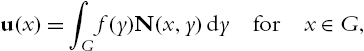
BogGf(x)=∫Gf(y)(x−y|x−y|d∫∞|x−y|ω(y+ζx−y|x−y|)ζd−1dζ)dy

for x∈G![]() . Here ω is any (nonnegative) function in C∞0(B)
. Here ω is any (nonnegative) function in C∞0(B)![]() with ∫Bωdx=1
with ∫Bωdx=1![]() , agrees with a singular integral operator, whose kernel fulfills (2.1.34)–(2.1.39), plus two operators enjoying stronger boundedness properties. If f∈C∞0(G)
, agrees with a singular integral operator, whose kernel fulfills (2.1.34)–(2.1.39), plus two operators enjoying stronger boundedness properties. If f∈C∞0(G)![]() it is easy to see that the same is true for BogGf
it is easy to see that the same is true for BogGf![]() using the representations
using the representations
BogGf(x)=∫Gf(y)(x−y)(x−y|x−y|d∫∞1ω(y+ζ(x−y))ζd−1dζ)dy=∫Gf(y)(x−y)(x−y|x−y|d∫∞0ω(y+ζ(x−y)|x−y|)(|x−y|ζ)d−1dζ)dy.

Setting u=BogGf![]() , we have
, we have
u(x)=∫Gf(y)N(x,y)dyforx∈G,
where
N(x,y)=x−y|x−y|d∫∞|x−y|ω(y+ζx−y|x−y|)ζd−1dζforx,y∈G.

By standard arguments we obtain (see [85, Proof of Lemma III.3.1] for more details)
∂jui(x)=∫Gf(y)∂jNi(x,y)dy+f(x)∫G(x−y)i(x−y)j|x−y|2ω(y)dy.

Computing ∂jN![]() we see that
we see that
∂jN=Kij(x,y)+Gij(x,y)
with
Kij(x,y)=δij|x−y|d∫∞0ω(x+ζx−y|x−y|)ζd−1dζ+xi−yi|x−y|d+1∫∞0∂jω(x+ζx−y|x−y|)ζddζ,
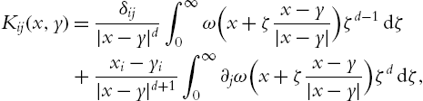
Gij(x,y)=xi−yi|x−y|d+1∫∞0∂jω(x+ζx−y|x−y|)d−1∑k=0(dk)|x−y|kζd−kdζ.

Now we want to justify the formula for a non-smooth function f. We claim that u∈W1,10(G)![]() , and
, and
∂ui∂xj=Hijffor a.e.x∈G,

where Hij![]() is the linear operator defined at f as
is the linear operator defined at f as
(Hijf)(x)=∫GKij(x,y)f(y)dy+∫GGij(x,y)f(y)dy+f(x)∫G(x−y)i(x−y)j|x−y|2ω(y)dyforx∈G,

for i,j=1,…d![]() . Here, Kij
. Here, Kij![]() is the kernel of a singular integral operator satisfying the same assumptions as the kernel K in Theorem 2.1.8. Moreover, the following holds
is the kernel of a singular integral operator satisfying the same assumptions as the kernel K in Theorem 2.1.8. Moreover, the following holds
|Gij(x,y)|⩽c|x−y|d−1forx,y∈Rd,x≠y.
Computing the divergence based on (2.1.76) and (2.1.77) we see that
divu=∫Gdf(y)∫∞1ω(y+r(x−y))rd−1drdy+∫Gf(y)d∑i=1∫∞1(xi−yi)∂iω(y+r(x−y))rddrdy+d∑i=1f(x)∫G(xi−yi)2|x−y|2ω(y)dy=∫Gdf(y)∫∞1ω(y+r(x−y))rd−1drdy+∫Gf(y)∫∞1ddrω(y+r(x−y))rddrdy+f(x)=−ω(x)∫Gf(y)dy+f(x)

using (2.1.74), (2.1.75) and ∫Gωdy=1![]() . As ∫Gfdy=0
. As ∫Gfdy=0![]() we obtain divu=f
we obtain divu=f![]() .
.
Now we pass to general functions f∈LA⊥(G)![]() . Recall that, if f∈C∞0,⊥(G)
. Recall that, if f∈C∞0,⊥(G)![]() , then u∈C∞0(G)
, then u∈C∞0(G)![]() , and moreover the equations (2.1.76) and (2.1.23) hold for every x∈G
, and moreover the equations (2.1.76) and (2.1.23) hold for every x∈G![]() . Due to (2.0.11), LA⊥(G)→LLogL⊥(G)
. Due to (2.0.11), LA⊥(G)→LLogL⊥(G)![]() , since B(t)
, since B(t)![]() grows at least linearly near infinity, and hence A(t)
grows at least linearly near infinity, and hence A(t)![]() dominates the function tlog(1+t)
dominates the function tlog(1+t)![]() near infinity. Since the space C∞0,⊥(G)
near infinity. Since the space C∞0,⊥(G)![]() is dense in LlogL⊥(G)
is dense in LlogL⊥(G)![]() , there exists a sequence of functions {fk}⊂C∞0,⊥(G)
, there exists a sequence of functions {fk}⊂C∞0,⊥(G)![]() such that fk→f
such that fk→f![]() in LlogL(G)
in LlogL(G)![]() . Hence
. Hence
BogG:LlogL(G)→L1(G)
(in fact, BogG![]() is also bounded into LlogL(G)
is also bounded into LlogL(G)![]() ). Furthermore,
). Furthermore,
Hij:LlogL(G)→L1(G),
as a consequence of (2.1.78) and of a special case of Theorem 2.1.9, with LA(G)=LlogL(G)![]() and LB(G)=L1(G)
and LB(G)=L1(G)![]() . Thus, Bogfk→BogGf
. Thus, Bogfk→BogGf![]() in L1(G)
in L1(G)![]() and Hijfk→Hijf
and Hijfk→Hijf![]() in L1(G)
in L1(G)![]() . This implies that u∈W1,10(G)
. This implies that u∈W1,10(G)![]() , and (2.1.76) and (2.1.23) hold.
, and (2.1.76) and (2.1.23) hold.
By Theorem 2.1.9, the singular integral operator defined by the first term on the right-hand side of (2.1.77) is bounded from LA(G)![]() into LB(G)
into LB(G)![]() . By inequality (2.1.78), the operator defined by the second term on the right-hand-side of (2.1.77) has (at least) the same boundedness properties as a Riesz potential operator with kernel 1|x−y|d−1
. By inequality (2.1.78), the operator defined by the second term on the right-hand-side of (2.1.77) has (at least) the same boundedness properties as a Riesz potential operator with kernel 1|x−y|d−1![]() . Such an operator is bounded in L1(G)
. Such an operator is bounded in L1(G)![]() and in L∞(G)
and in L∞(G)![]() , with norms depending only on |G|
, with norms depending only on |G|![]() and on d. An interpolation theorem by Calderon [19, Theorem 2.12, Chap. 3] then ensures that it is also bounded from LA(G)
and on d. An interpolation theorem by Calderon [19, Theorem 2.12, Chap. 3] then ensures that it is also bounded from LA(G)![]() into LA(G)
into LA(G)![]() , and hence from LA(G)
, and hence from LA(G)![]() into LB(G)
into LB(G)![]() , with norm depending on d and |G|
, with norm depending on d and |G|![]() . Finally, the operator given by the last term on the right-hand-side of (2.1.77) is pointwise bounded (in absolute value) by |f(x)|
. Finally, the operator given by the last term on the right-hand-side of (2.1.77) is pointwise bounded (in absolute value) by |f(x)|![]() . Thus, it is bounded from LA(G)
. Thus, it is bounded from LA(G)![]() into LA(G)
into LA(G)![]() , and hence from LA(G)
, and hence from LA(G)![]() into LB(G)
into LB(G)![]() . Equations (2.1.21) and (2.1.24) are thus established.
. Equations (2.1.21) and (2.1.24) are thus established.
Inequality (2.1.25) follows from (2.1.24) via a scaling argument analogous to that which leads to (2.1.42) from (2.1.41) – see the Proof of Theorem 2.1.9. □
Proof of Theorem 2.1.7
By an argument as in the proofs of [85, Lemmas 3.4 and 3.5, and Theorem 3.3], it suffices to show that, if G and G are bounded Lipschitz domains, for which the domain G0=G∩D![]() is star-shaped with respect to a ball B⋐G0
is star-shaped with respect to a ball B⋐G0![]() , and f has the form
, and f has the form
f=ζdivg+θ∫Gφdivgdy,

for some functions ζ∈C∞0(G)![]() , θ∈C∞0(G0)
, θ∈C∞0(G0)![]() and φ∈C∞(‾G)
and φ∈C∞(‾G)![]() , and fulfills
, and fulfills
∫G0f(x)dx=0,

then there exists a function w∈W1,B0(G)![]() such that
such that
divw=finG0,
‖∇w‖LB(G0)⩽C‖divg‖LA(G),
and
‖w‖LB(G0)⩽C‖g‖LA(G),
for some constant C=C(φ,θ,ζ,c,B,G,G)![]() , where c is the constant appearing in (2.0.11) and (2.0.12).
, where c is the constant appearing in (2.0.11) and (2.0.12).
Since f∈LA⊥(G0)![]() , an inspection of the proof of Theorem 2.1.6 then reveals that the function w, given by
, an inspection of the proof of Theorem 2.1.6 then reveals that the function w, given by
w(x)=∫G0f(y)N(x,y)dyforx∈G0,

where
N(x,y)=x−y|x−y|d∫∞|x−y|ω(y+ζx−y|x−y|)ζd−1dζforx,y∈G,

and ω is any (nonnegative) function in C∞0(B)![]() with ∫Bωdx=1
with ∫Bωdx=1![]() , satisfies (2.1.79), and
, satisfies (2.1.79), and
‖∇w‖LB(G0)⩽C‖f‖LA(G0)
for some constant C. Since
‖f‖LA(G0)⩽C‖divg‖LA(G)
for some constant C, inequality (2.1.80) follows. It remains to prove (2.1.81). To this purpose, assume, for the time being, that divg∈C∞0(G)![]() . Then, by [85, Equation 3.35],
. Then, by [85, Equation 3.35],
wi(x)=−∫G0Ni(x,y)g(y)⋅∇ζ(y)dy−∫G0Kij(x,x−y)ζ(y)gj(y)dy−∫G0n∑j=1Gij(x,y)ζ(y)gj(y)dy−ζ(x)d∑j=1gj(x)∫G0(xi−yi)(xj−yj)|x−y|2ω(y)dy−(∫Gg⋅∇φdy)∫G0Ni(x,y)θ(y)dyfor a.e.x∈G0,

where the kernels Kij![]() and Gij
and Gij![]() satisfy the same assumptions as the kernels in (2.1.77), and |N(x,y)|⩽C|x−y|1−d
satisfy the same assumptions as the kernels in (2.1.77), and |N(x,y)|⩽C|x−y|1−d![]() for some constant C. Note that condition (2.1.28) has been used in writing the last term on the right-hand side of equation (2.1.86).
for some constant C. Note that condition (2.1.28) has been used in writing the last term on the right-hand side of equation (2.1.86).
We now drop the assumption that divg∈C∞0(G)![]() . Condition (2.0.11) entails that LA(G)→LlogL(G)
. Condition (2.0.11) entails that LA(G)→LlogL(G)![]() , and hence HA0(G)→HLlogL0(G)
, and hence HA0(G)→HLlogL0(G)![]() , where the latter space denotes HA0(G)
, where the latter space denotes HA0(G)![]() with A(t)
with A(t)![]() equivalent to tlog(1+t)
equivalent to tlog(1+t)![]() near infinity. Thus, g∈HLlogL0(G)
near infinity. Thus, g∈HLlogL0(G)![]() , and hence it can be approximated by a sequence of functions {gk}⊂C∞0(G)
, and hence it can be approximated by a sequence of functions {gk}⊂C∞0(G)![]() in such a way that gk→g
in such a way that gk→g![]() in HLlogL(G)
in HLlogL(G)![]() , cf. Theorem A.1.46. The first and third term on the right-hand side of (2.1.86) are integral operators applied to g whose kernel is bounded by a multiple of |x−y|1−d
, cf. Theorem A.1.46. The first and third term on the right-hand side of (2.1.86) are integral operators applied to g whose kernel is bounded by a multiple of |x−y|1−d![]() . The fourth term is just bounded by a constant multiple of |g|
. The fourth term is just bounded by a constant multiple of |g|![]() . The last term is a constant multiple of an integral of g against a bounded vector-valued function ∇φ. Hence, all these operators are bounded from LA(G)
. The last term is a constant multiple of an integral of g against a bounded vector-valued function ∇φ. Hence, all these operators are bounded from LA(G)![]() into LA(G0)
into LA(G0)![]() . The second term is a singular integral operator enjoying the same properties as the singular integral operator K in Theorems 2.1.8 and 2.1.9. Thus, since all operators appearing on the right-hand side of (2.1.86) are bounded from LlogL(G)
. The second term is a singular integral operator enjoying the same properties as the singular integral operator K in Theorems 2.1.8 and 2.1.9. Thus, since all operators appearing on the right-hand side of (2.1.86) are bounded from LlogL(G)![]() into L1(G0)
into L1(G0)![]() , the right-hand side of (2.1.86), evaluated with g replaced by gk
, the right-hand side of (2.1.86), evaluated with g replaced by gk![]() , converges in L1(G0)
, converges in L1(G0)![]() to the right-hand-side of (2.1.86). On the other hand, equation (2.1.82) and the properties of the Bogovskiĭ operator tell us that the left-hand-side of (2.1.86), with wi
to the right-hand-side of (2.1.86). On the other hand, equation (2.1.82) and the properties of the Bogovskiĭ operator tell us that the left-hand-side of (2.1.86), with wi![]() corresponding to gk
corresponding to gk![]() , converges in L1(G0)
, converges in L1(G0)![]() to the left-hand-side of (2.1.86). Altogether, we conclude that (2.1.86) actually holds even if g is just in HA0(G)
to the left-hand-side of (2.1.86). Altogether, we conclude that (2.1.86) actually holds even if g is just in HA0(G)![]() .
.
The properties of the operators on the right-hand-side of (2.1.86) mentioned above ensure that they are bounded from LA(G)![]() into LB(G0)
into LB(G0)![]() . Inequality (2.1.81) thus follows from (2.1.86). □
. Inequality (2.1.81) thus follows from (2.1.86). □
2.2 Negative norms & the pressure
We need a last preliminary result in preparation of the proof of Theorem 2.0.5.
Proposition 2.2.1

Note that equation (2.2.87) is well known under the assumption that A∈∇2![]() near infinity, namely ˜A∈Δ2
near infinity, namely ˜A∈Δ2![]() near infinity. This is because C∞0(G)
near infinity. This is because C∞0(G)![]() is dense in L˜A(G)
is dense in L˜A(G)![]() in this case. Equation (2.2.88) also easily follows from this property when A∈∇2
in this case. Equation (2.2.88) also easily follows from this property when A∈∇2![]() near infinity. The novelty of Proposition 2.2.1 is in the arbitrariness of A.
near infinity. The novelty of Proposition 2.2.1 is in the arbitrariness of A.
Proof of Proposition 2.2.1
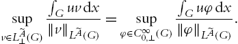
Consider first (2.2.87). It clearly suffices to show that
supv∈L˜A(G)∫Guvdx‖v‖L˜A(G)=supv∈L∞(G)∫Guvdx‖v‖L˜A(G),

and
supv∈L∞(G)∫Guvdx‖v‖L˜A(G)=supφ∈C∞0(G)∫Guφdx‖φ‖L˜A(G).

Given any v∈L˜A(G)![]() , define, for k∈N
, define, for k∈N![]() , the function vk:G→R
, the function vk:G→R![]() as
as
vk=sign(v)min{|v|,k}.
Clearly, vk∈L∞(G)![]() , and 0⩽|vk|↗|v|
, and 0⩽|vk|↗|v|![]() a.e. in G as k→∞
a.e. in G as k→∞![]() . Hence,
. Hence,
∫G|uvk|dx↗∫G|uv|dxask→∞,

by the monotone convergence theorem for integrals, and, by the Fatou property of the Luxemburg norm,
‖vk‖L˜A(G)↗‖v‖L˜A(G)ask→∞.
Thus, since
supv∈L˜A(G)∫Guvdx‖v‖L˜A(G)=supv∈L˜A(G)∫G|uv|dx‖v‖L˜A(G),

equation (2.2.89) follows.
As far as (2.2.90) is concerned, consider an increasing sequence of compact sets Ek![]() such that dist(Ek,Rd∖G)⩾2k
such that dist(Ek,Rd∖G)⩾2k![]() , Ek⊂Ek+1⊂G
, Ek⊂Ek+1⊂G![]() for k∈N
for k∈N![]() , and ∪kEk=G
, and ∪kEk=G![]() . Moreover, let {ϱk}
. Moreover, let {ϱk}![]() be a family of (nonnegative) smooth mollifiers in Rd
be a family of (nonnegative) smooth mollifiers in Rd![]() , such that suppϱk⊂B1k(0)
, such that suppϱk⊂B1k(0)![]() and ∫Rdϱkdx=1
and ∫Rdϱkdx=1![]() for k∈N
for k∈N![]() . Given v∈L∞(G)
. Given v∈L∞(G)![]() , define wk:Rd→R
, define wk:Rd→R![]() as
as
wk={vin Ek,0elsewhere,

and φk:Rd→R![]() as
as
φk(x)=∫Rdwk(y)ϱk(x−y)dyforx∈Rd.

Classical properties of mollifiers ensure that
φk∈C∞0(G),φk→va.e. in G ask→∞,‖φk‖L∞(G)⩽‖v‖L∞(G)fork∈N.

Thus, if u∈LA(G)![]() , then
, then
∫Guφkdx→∫Guvdxask→∞,

by the dominated convergence theorem for integrals. Moreover,
‖φk‖L˜A(G)→‖v‖L˜A(G)ask→∞.
Indeed, by dominated convergence and the definition of Luxemburg norm,
∫G˜A(|φk|‖v‖L˜A(G))dx→∫G˜A(|v|‖v‖L˜A(G))dx⩽1ask→∞.

In particular, for every ε>0![]() , there exists kε
, there exists kε![]() such that
such that
∫G˜A(|φk|‖v‖L˜A(G))dx<1+εifk>kε.

Hence, by the arbitrariness of ε and the definition of Luxemburg norm,
liminfk→∞‖φk‖L˜A(G)⩾‖v‖L˜A(G).
We also have that
limsupk→∞‖φk‖L˜A(G)⩽‖v‖L˜A(G).
Indeed, assume that (2.2.96) fails. Then, there exists σ>0![]() and a subsequence of {φk}
and a subsequence of {φk}![]() , still denoted by {φk}
, still denoted by {φk}![]() , such that
, such that
1<∫G˜A(|φk|‖v‖L˜A(G)+σ)dx→∫G˜A(|v|‖v‖L˜A(G)+σ)dx⩽1,

which is a contradiction. Equation (2.2.94) follows from (2.2.95) and (2.2.96). Coupling (2.2.93) with (2.2.94) implies (2.2.90). The proof of (2.2.87) is complete.
The proof of (2.2.88) follows along the same lines, and, in particular, via the equations
supv∈L˜A⊥(G)∫Guvdx‖v‖L˜A(G)=supv∈L∞⊥(G)∫Guvdx‖v‖L˜A(G),

and
supv∈L∞⊥(G)∫Guvdx‖v‖L˜A(G)=supφ∈C∞0,⊥(G)∫Guφdx‖φ‖L˜A(G).

For any v∈L˜A⊥(G)![]() , we define the sequence of functions {‾vk}⊂L∞⊥(G)
, we define the sequence of functions {‾vk}⊂L∞⊥(G)![]() by
by
‾vk=vk−(vk)G.
Here we have k∈N![]() and vk
and vk![]() is given by (2.2.91). We can prove equation (2.2.97) via a slight variant of the argument used for (2.2.89). Here, one has to use the fact that (vk)G→0
is given by (2.2.91). We can prove equation (2.2.97) via a slight variant of the argument used for (2.2.89). Here, one has to use the fact that (vk)G→0![]() as k→∞
as k→∞![]() .
.
Equation (2.2.98) can be established similarly to (2.2.90). Let v∈L∞⊥(G)![]() be given. We have to replace the sequence {φk}
be given. We have to replace the sequence {φk}![]() defined by (2.2.92) with the sequence {‾φk}⊂C∞0,⊥(G)
defined by (2.2.92) with the sequence {‾φk}⊂C∞0,⊥(G)![]() defined by
defined by
‾φk=φk−(φk)Gψfork∈N.
Here ψ is any function in C∞0(G)![]() such that ∫Gψdx=1
such that ∫Gψdx=1![]() . For every ε>0
. For every ε>0![]() , there exists kε∈N
, there exists kε∈N![]() such that ‖‾φk‖L∞(G)⩽‖v‖L∞(G)+ε
such that ‖‾φk‖L∞(G)⩽‖v‖L∞(G)+ε![]() , provided that k>kε
, provided that k>kε![]() . □
. □
Proof of Theorem 2.0.5
Let u∈L1(G)![]() . Then
. Then
‖u−uG‖LB(G)=supv∈L˜B(G)∫G(u−uG)vdx‖v‖L˜B(G)=supv∈L˜B(G)∫G(u−uG)(v−vG)dx‖v‖L˜B(G)=supv∈L˜B(G)∫Gu(v−vG)dx‖v‖L˜B(G)⩽3supv∈L˜B(G)∫Gu(v−vG)dx‖v−vG‖L˜B(G)=3supv∈L˜B⊥(G)∫Guvdx‖v‖L˜B(G)=3supφ∈C∞0,⊥(G)∫Guφdx‖φ‖L˜B(G).

Note that the inequality in (2.2.99) holds since, by the first inequality in (1.2.3),
‖v−vG‖L˜B(G)⩽‖v‖L˜B(G)+‖vG‖L˜B(G)⩽‖v‖L˜B(G)+|vG|‖1‖L˜B(G)⩽‖v‖L˜B(G)+2|G|‖v‖L˜B(G)‖1‖LB(G)‖1‖L˜B(G)=‖v‖L˜B(G)+2|G|‖v‖L˜B(G)1B−1(|G|)1˜B−1(|G|)⩽3‖v‖L˜B(G).

The last equality in (2.2.99) follows from (2.2.88). By Theorem 2.1.6, applied with A and B replaced with ˜B![]() and ˜A
and ˜A![]() , respectively, there exists a constant C=C(G,c)
, respectively, there exists a constant C=C(G,c)![]() such that
such that
supφ∈C∞0,⊥(G)∫Guφdx‖φ‖L˜B(G)=supφ∈C∞0,⊥(G)∫Gudiv(BogGφ)dx‖φ‖L˜B(G)⩽Csupφ∈C∞0,⊥(G)∫Gudiv(BogGφ)dx‖∇BogGφ‖L˜A(G)⩽Csupφ∈C∞0(G)∫Gudivφdx‖∇φ‖L˜A(G)dx=C‖u‖W−1,A(G).
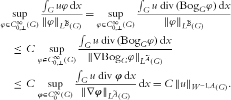
The first inequality in (2.0.13) follows from (2.2.99) and (2.2.100). The second inequality is trivial, since
‖u‖W−1,A(G)=supφ∈C∞0(G)∫Gudivφ‖∇φ‖L˜A(G)dx=supφ∈C∞0(G)∫G(u−uG)divφdx‖∇φ‖L˜A(G)⩽Csupφ∈C∞0(G)∫G(u−uG)divφdx‖divφ‖L˜A(G)dx⩽Csupφ∈C∞0,⊥(G)∫G(u−uG)φdx‖φ‖L˜A(G)dx⩽2C‖u−uG‖LA(G),

for some constant C=C(d)![]() . □
. □
In the remaining part of this section, we focus on the second question raised in the introduction of this chapter, namely the reconstruction of the pressure π in a correct Orlicz space. In case of fluids governed by a general constitutive law, the function H belongs to some Orlicz space LA(G)![]() . If A∈Δ2∩∇2
. If A∈Δ2∩∇2![]() , then π∈LA(G)
, then π∈LA(G)![]() as well. However, in general, one can only expect that π belongs to some larger Orlicz space LB(G)
as well. However, in general, one can only expect that π belongs to some larger Orlicz space LB(G)![]() . The balance between the Young functions A and B is determined by conditions (2.0.11) and (2.0.12), as stated in the following result.
. The balance between the Young functions A and B is determined by conditions (2.0.11) and (2.0.12), as stated in the following result.
Theorem 2.2.10
Let A and B be Young functions fulfilling (2.0.11) and (2.0.12). Let G be a bounded domain with the cone property in Rd![]() , d⩾2
, d⩾2![]() . Assume that H∈LA(G)
. Assume that H∈LA(G)![]() satisfies
satisfies
∫GH:∇φdx=0

for every φ∈C∞0,div(G)![]() . Then there exists a unique function π∈LB⊥(G)
. Then there exists a unique function π∈LB⊥(G)![]() such that
such that
∫GH:∇φdx=∫Gπdivφdx

for every φ∈C∞0(G)![]() . Moreover, there exists a constant C=C(G,c)
. Moreover, there exists a constant C=C(G,c)![]() such that
such that
‖π‖LB(G)⩽C‖H−HG‖LA(G),
and
∫GB(|π|)dx⩽∫GA(C|H−HG|)dx.
Here, c denotes the constant appearing in (2.0.11) and (2.0.12).
In particular, Theorem 2.2.10 reproduces, within a unified framework, various results appearing in the literature. For instance, when the power law model is in force, the function A(t)![]() is just a power tq
is just a power tq![]() for some q>1
for some q>1![]() . So LA(G)
. So LA(G)![]() agrees with the Lebesgue space Lq(G)
agrees with the Lebesgue space Lq(G)![]() , and Theorem 2.2.10 recovers the fact that π belongs to the same Lebesgue space Lq(G)
, and Theorem 2.2.10 recovers the fact that π belongs to the same Lebesgue space Lq(G)![]() .
.
As far as the simplified system (without convective term) for the Eyring–Prandtl model (see Chapter 4) is concerned, under appropriate assumptions on the function f one has that H=S(ε(v))+∇Δ−1f∈expL(G)![]() . Hence, via Theorem 2.2.10, we obtain the existence of a pressure π∈expL12(G)
. Hence, via Theorem 2.2.10, we obtain the existence of a pressure π∈expL12(G)![]() . More generally, if H∈expLβ(G)
. More generally, if H∈expLβ(G)![]() for some β>0
for some β>0![]() , one has that π∈expLβ/(β+1)(G)
, one has that π∈expLβ/(β+1)(G)![]() . The complete system for the Eyring–Prandtl model, in the 2-dimensional case, admits a weak solution v such that v⊗v∈LlogL2(G)
. The complete system for the Eyring–Prandtl model, in the 2-dimensional case, admits a weak solution v such that v⊗v∈LlogL2(G)![]() and hence H=S(ε(v))+∇Δ−1f−v⊗v∈LlogL2(G)
and hence H=S(ε(v))+∇Δ−1f−v⊗v∈LlogL2(G)![]() , see Chapter 4. Again, one cannot expect that the pressure π belongs to the same space. In fact, Theorem 2.2.10 implies the existence of a pressure π∈LlogL(G)
, see Chapter 4. Again, one cannot expect that the pressure π belongs to the same space. In fact, Theorem 2.2.10 implies the existence of a pressure π∈LlogL(G)![]() . This reproduces a result from [33]. In general, if H∈LlogLα(G)
. This reproduces a result from [33]. In general, if H∈LlogLα(G)![]() for some α⩾1
for some α⩾1![]() , then we obtain that π∈LlogLα−1(G)
, then we obtain that π∈LlogLα−1(G)![]() .
.
Proof of Theorem 2.2.10
By De Rahms Theorem, in the version of [131], there exists a distribution Ξ such that
∫GH:∇φdx=Ξ(divφ)
for every φ∈C∞0(G)![]() . Replacing φ with BogG(φ−φG)
. Replacing φ with BogG(φ−φG)![]() in (2.2.104), where φ∈C∞0(G)
in (2.2.104), where φ∈C∞0(G)![]() , implies
, implies
∫GH:∇BogG(φ−φG)dx=Ξ(φ−φG)

for every φ∈C∞0(G)![]() . We claim that the linear functional C∞0(G)∋φ↦Ξ(φ−φG)
. We claim that the linear functional C∞0(G)∋φ↦Ξ(φ−φG)![]() is bounded on C∞0(G)
is bounded on C∞0(G)![]() equipped with the L∞(G)
equipped with the L∞(G)![]() norm. Indeed, by (2.0.11), one has that LA(G)→LlogL(G)
norm. Indeed, by (2.0.11), one has that LA(G)→LlogL(G)![]() . Moreover, by a special case of Theorem 2.1.6, ∇BogG:L∞⊥(G)→expL(G)
. Moreover, by a special case of Theorem 2.1.6, ∇BogG:L∞⊥(G)→expL(G)![]() . Thus, since LlogL(G)
. Thus, since LlogL(G)![]() and expL(G)
and expL(G)![]() are Orlicz spaces generated by Young functions which are conjugate of each other,
are Orlicz spaces generated by Young functions which are conjugate of each other,
|∫GH:∇BogG(φ−φG)dx|⩽C‖H‖LlogL(G)‖∇BogG(φ−φ)G)‖expL(G)⩽C′‖H‖LA(G)‖φ−φG‖L∞(G)⩽C″‖H‖LA(G)‖φ‖L∞(G),

for every φ∈C∞0(G)![]() , where C=C(|G|,d)
, where C=C(|G|,d)![]() and C′=C′(G,c)
and C′=C′(G,c)![]() . Hence, the relevant functional can be continued to a bounded linear functional on φ∈C0(G)
. Hence, the relevant functional can be continued to a bounded linear functional on φ∈C0(G)![]() , with the same norm.
, with the same norm.
Now, as a consequence of Riesz's representation Theorem, there exists a Radon measure μ such that
Ξ(φ−φG)=∫Gφdμ

for every φ∈C0(G)![]() . Fix any open set E⊂G
. Fix any open set E⊂G![]() . By Theorem 2.1.6 again, there exists a constant C such that
. By Theorem 2.1.6 again, there exists a constant C such that
μ(E)=supφ∈C00(E),‖φ‖∞=1Ξ(φ−φG)=supφ∈C00(E),‖φ‖∞=1∫GH:∇BogG(φ−φG)dx⩽supφ∈C00(E),‖φ‖∞=1‖H‖LlogL(E)‖∇BogG(φ−φG)‖expL(G)⩽Csupφ∈C00(E),‖φ‖∞=1‖H‖LlogL(E)‖φ−(φ)G‖L∞(G)⩽C‖H‖LlogL(E).

One can verify that the norm ‖⋅‖LlogL(E)![]() is absolutely continuous in the following sense. For every ε>0
is absolutely continuous in the following sense. For every ε>0![]() there exists δ>0
there exists δ>0![]() such that ‖H‖LlogL(E)<ε
such that ‖H‖LlogL(E)<ε![]() if |E|<δ
if |E|<δ![]() . Since any Lebesgue measurable set can be approximated from outside by open sets, inequality (2.2.106) implies that the measure μ is absolutely continuous with respect to the Lebesgue measure. Hence, μ has a density with respect to the Lebesgue measure. So Ξ can be represented by a function π∈L1(G)
. Since any Lebesgue measurable set can be approximated from outside by open sets, inequality (2.2.106) implies that the measure μ is absolutely continuous with respect to the Lebesgue measure. Hence, μ has a density with respect to the Lebesgue measure. So Ξ can be represented by a function π∈L1(G)![]() fulfilling (2.2.101) holds. The function π is uniquely determined if we assume that πG=0
fulfilling (2.2.101) holds. The function π is uniquely determined if we assume that πG=0![]() . By this assumption, Theorem 2.0.5, and equation (2.2.101) we have that
. By this assumption, Theorem 2.0.5, and equation (2.2.101) we have that
‖π‖LB(G)⩽C‖∇π‖W−1,A(G)=Csupφ∈C∞0(G)∫Gπdivφdx‖∇φ‖L˜A(G)=Csupφ∈C∞0(G)∫GH:∇φdx‖∇φ‖L˜A(G)=Csupφ∈C∞0(G)∫G(H−HG):∇φdx‖∇φ‖L˜A(G)⩽2C‖H−HG‖LA(G),

where C=C(G,c)![]() . This proves inequality (2.2.102). Inequality (2.2.103) follows from (2.2.102), by replacing A and B with kA and kB, respectively, with k=1∫GA(|H−HG|)dx
. This proves inequality (2.2.102). Inequality (2.2.103) follows from (2.2.102), by replacing A and B with kA and kB, respectively, with k=1∫GA(|H−HG|)dx![]() , via an argument analogous to that of the proof of (2.1.42). □
, via an argument analogous to that of the proof of (2.1.42). □
2.3 Sharp conditions for Korn-type inequalities
In order to formulate the main result of this section we need to introduce the Banach function space
EA(G):={u∈LA(G):ε(u)∈LA(G)},‖u‖EA(G):=‖u‖LA(G)+‖ε(u)‖LA(G),

and its subspace
EA0(G):={u∈EA(G): the continuation of u by zero belongs to EA(Rd)}.
If A is of power growth (belongs to Δ2∩∇2![]() ) then there is no need for this definition. In this case the space EA(G)
) then there is no need for this definition. In this case the space EA(G)![]() coincides with the standard Lebesgue spaces (Orlicz spaces). However, this is not true in our general context.
coincides with the standard Lebesgue spaces (Orlicz spaces). However, this is not true in our general context.
Theorem 2.3.11
Let G be any open bounded set in Rd![]() . Let A and B be Young functions such that
. Let A and B be Young functions such that
t∫tt0B(s)s2ds⩽A(ct)fort⩾t0,

and
t∫tt0˜A(s)s2ds⩽˜B(ct)fort⩾t0,

for some constants c>0![]() and t0⩾0
and t0⩾0![]() . Then EA0(G)⊂W1,B0(G)
. Then EA0(G)⊂W1,B0(G)![]() , and
, and
‖∇u‖LB(G)⩽C‖ε(u)‖LA(G)
for some constant C=C(t0,G,c,A,B)![]() and for every u∈EA0(G)
and for every u∈EA0(G)![]() . Moreover,
. Moreover,
∫GB(C|∇u|)dx⩽C1+∫GA(C|ε(u)|)dx

for every u∈EA0(G)![]() with C1=C1(t0,G,c,A,B)
with C1=C1(t0,G,c,A,B)![]() . If t0=0
. If t0=0![]() then C1=0
then C1=0![]() and C=C(G,c)
and C=C(G,c)![]() .
.
Theorem 2.3.12
Let G be an open bounded Lipschitz domain in Rd![]() . Assume that A and B are Young functions fulfilling conditions (2.3.107) and (2.3.108). Then EA(G)⊂W1,B(G)
. Assume that A and B are Young functions fulfilling conditions (2.3.107) and (2.3.108). Then EA(G)⊂W1,B(G)![]() , and
, and
‖∇u−(∇u)G‖LB(G)⩽C‖ε(u)−(ε(u))G‖LA(G)
for some constant C=C(t0,G,c;A,B)![]() and for every u∈EA(G)
and for every u∈EA(G)![]() . Moreover,
. Moreover,
∫GB(C|∇u−(∇u)G|)dx⩽C1+∫GA(C|ε(u)−(ε(u))G|)dx

for every u∈EA(G)![]() with C1=C1(t0,G,c,A,B)
with C1=C1(t0,G,c,A,B)![]() . If t0=0
. If t0=0![]() then C1=0
then C1=0![]() and C=C(G,c)
and C=C(G,c)![]() .
.
Instead of subtracting the mean value it is also useful to subtract an element from the kernel of the differential operator ε given by
R={w:Rd→Rd:w(x)=b+Qx:b∈Rd,Q∈Rd×d,Q=−QT}.
Corollary 2.3.1
Let G be an open bounded Lipschitz domain in Rd![]() . Assume that A and B are Young functions fulfilling conditions (2.3.107) and (2.3.108). Then EA(G)⊂W1,B(G)
. Assume that A and B are Young functions fulfilling conditions (2.3.107) and (2.3.108). Then EA(G)⊂W1,B(G)![]() , and there is w∈R
, and there is w∈R![]() such that
such that
‖∇u−∇w‖LB(G)⩽C‖ε(u)‖LA(G)
for some constant C=C(t0,G,c;A,B)![]() and for every u∈EA(G)
and for every u∈EA(G)![]() . Moreover,
. Moreover,
∫GB(C|∇u−∇w|)dx⩽C1+∫GA(C|ε(u)|)dx

for every u∈EA(G)![]() with C1=C1(t0,G,c,A,B)
with C1=C1(t0,G,c,A,B)![]() . If t0=0
. If t0=0![]() then C1=0
then C1=0![]() and C=C(G,c)
and C=C(G,c)![]() .
.
Theorem 2.3.13

Proof of Theorem 2.3.12
Let us introduce negative norms for single partial derivatives as follows. Given u∈L1(G)![]() , we set
, we set
‖∂u∂xk‖W−1,A(G)=supφ∈C∞0(G)∫Gu∂φ∂xkdx‖∇φ‖L˜A(G)fork=1,…,d.

Obviously, the following holds
‖∂u∂xk‖W−1,A(G)⩽‖∇u‖W−1,A(G)fork=1,…d.
On the other hand,
‖∇u‖W−1,A(G)=supφ∈C∞0(G)∫Gudivφdx‖∇φ‖L˜A(G)=supφ∈C∞0(G)d∑k=1∫Gu∂φk∂xkdx‖∇φ‖L˜A(G)⩽supφ∈C∞0(G)d∑k=1∫Gu∂φk∂xkdx‖∇φk‖L˜A(G)⩽d∑k=1supφ∈C∞0(G)∫Gu∂φ∂xkdx‖∇φ‖L˜A(G)=d∑k=1‖∂u∂xk‖W−1,A(G),

where φk![]() denotes the k-th component of φ. Next, notice the identity
denotes the k-th component of φ. Next, notice the identity
∂2vi∂xk∂xj=∂(ε(v))ij∂xk+∂(ε(v))ik∂xj−∂(ε(v))jk∂xi

for every weakly differentiable function v:G→Rd![]() . Thus, the following chain holds for every u∈W1,1(G)∩EA(G)
. Thus, the following chain holds for every u∈W1,1(G)∩EA(G)![]()
‖∇u−(∇u)G‖LB(G)⩽Cd∑i,j=1‖∂ui∂xj−(∂ui∂xj)G‖LB(G)⩽Cn∑i,j=1‖∇∂ui∂xj‖W−1,A(G)⩽Cd∑i,j,k=1‖∂2ui∂xk∂xj‖W−1,A(G)⩽Cd∑i,j,k=1(‖∂(ε(u))ij∂xk‖W−1,A(G)+‖∂(ε(u))ik∂xj‖W−1,A(G)+‖∂(ε(u))jk∂xi‖W−1,A(G))⩽Cd∑i,j=1‖∇(ε(u))ij‖W−1,A(G)⩽Cn∑i,j=1‖(ε(u))ij−((ε(u))ij)G‖LA(G)⩽C‖ε(u)−(ε(u))G‖LA(G).
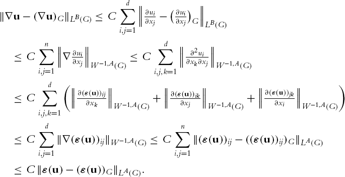
Note that the second inequality holds by Theorem 2.0.5 (see Remark 2.0.6 for the case t0>0![]() ), the third by (2.3.117), the fourth by (2.3.118), the fifth by (2.3.116), and the sixth by Theorem 2.0.5 again.
), the third by (2.3.117), the fourth by (2.3.118), the fifth by (2.3.116), and the sixth by Theorem 2.0.5 again.
Let us turn to the modular version. Suppose first that t0=0![]() in (2.3.107) and (2.3.108). An inspection of the proof of Theorem (2.3.119) and of the statement of Theorem 2.0.5 tells us that the constant C in (2.3.119) depends only on G and on the constant c appearing in conditions (2.3.107) and (2.3.108). These conditions continue to hold if the functions A and B are replaced by the functions AM
in (2.3.107) and (2.3.108). An inspection of the proof of Theorem (2.3.119) and of the statement of Theorem 2.0.5 tells us that the constant C in (2.3.119) depends only on G and on the constant c appearing in conditions (2.3.107) and (2.3.108). These conditions continue to hold if the functions A and B are replaced by the functions AM![]() and BM
and BM![]() given by AM(t)=A(t)/M
given by AM(t)=A(t)/M![]() and BM(t)=B(t)/M
and BM(t)=B(t)/M![]() for some positive constant M. Given a function u∈EA0(G)
for some positive constant M. Given a function u∈EA0(G)![]() , set
, set
M=∫ΩA(C|ε(u)−(ε(u))G|)dx.
If M=∞![]() , then inequality (2.3.111) holds trivially. We may thus assume that
, then inequality (2.3.111) holds trivially. We may thus assume that
‖∇u−(∇u)G‖LAM(G)⩽1.
Hence, by inequality (2.3.110) applied with A and B replaced by AM![]() and BM
and BM![]() , we obtain
, we obtain
∫ΩB(|∇u−(∇u)G|)dx⩽∫ΩA(C|ε(u)−(ε(u))G|)dx.

This is (2.3.111) with C1=0![]() .
.
Assume next that (2.3.107) and (2.3.108) just hold for some t0>0![]() . The functions A and B can be replaced by new Young functions ‾A
. The functions A and B can be replaced by new Young functions ‾A![]() and ‾B
and ‾B![]() , equivalent to A and B near infinity, and such that (2.3.107) and (2.3.108) hold for the new functions with t0=0
, equivalent to A and B near infinity, and such that (2.3.107) and (2.3.108) hold for the new functions with t0=0![]() . The same argument as above implies (2.3.120) with A and B replaced by ‾A
. The same argument as above implies (2.3.120) with A and B replaced by ‾A![]() and ‾B
and ‾B![]() ., i.e., we have
., i.e., we have
∫Ω‾B(|∇u−(∇u)G|)dx⩽∫Ω‾A(C|ε(u)−(ε(u))G|)dx

for some constant C. Since ‾A![]() and ‾B
and ‾B![]() are equivalent to A and B near infinity, there exist constants t0>0
are equivalent to A and B near infinity, there exist constants t0>0![]() and c>0
and c>0![]() such that
such that
‾A(t)⩽A(ct)ift⩾t0,B(t)⩽‾B(ct)ift⩾t0.
From (2.3.121) and (2.3.122) we obtain
∫GB(|∇u−(∇u)G|)dx=∫{|∇u−(∇u)G|<t0}B(|∇u−(∇u)G|)dx+∫{|∇u−(∇u)G|⩾t0}B(|∇u−(∇u)G|)dx⩽B(t0)|G|+∫G‾B(c|∇u−(∇u)G|)dx⩽B(t0)|G|+∫G‾A(Cc|ε(u)−(ε(u))G|)dx⩽B(t0)|G|+∫{Cc|ε(u)−(ε(u))G|<t0}‾A(Cc|ε(u)−(ε(u))G|)dx+∫{Cc|ε(u)−(ε(u))G|⩾t0}‾A(Cc|ε(u)−(ε(u))G|)dx⩽(B(t0)+A(ct0))|G|+∫GA(Cc2|ε(u)−(ε(u))G|)dx,

namely (2.3.111) with C1=(B(t0)+A(ct0))|G|![]() . □
. □
Proof of Theorem 2.3.11
If u∈W1,10(G)![]() , then (∇u)G=(ε(u))G=0
, then (∇u)G=(ε(u))G=0![]() , and Theorem 2.3.11 implies the claim. □
, and Theorem 2.3.11 implies the claim. □
Proof of Corollary 2.3.1
Proof of Theorem 2.3.13
Step 1: Star-shaped domains.
First, we assume that G is star-shaped with respect to some ball B⊂G![]() . Then, according to formula (2.39) in [126] each v∈C∞(G)
. Then, according to formula (2.39) in [126] each v∈C∞(G)![]() can be represented as
can be represented as
u(x)=PGu(x)+Lε(ε(u))(x),
where PG:L1(G)→R![]() is a suitable linear projection operator into the space of rigid motions (compare (2.33)–(2.39) in [126]) defined even for L1(G)
is a suitable linear projection operator into the space of rigid motions (compare (2.33)–(2.39) in [126]) defined even for L1(G)![]() functions. Furthermore, the operator Lε
functions. Furthermore, the operator Lε![]() is a weakly singular integral operator (compare (2.37) in [126]) given by
is a weakly singular integral operator (compare (2.37) in [126]) given by
Lε(φ):=Sε(ψ)+Tε(ψ),ψ∈C∞(G),Siε(φ)(x):=∫GGi(x,e)|x−z|d−1:ψ(z)dz,i=1,...,d,Tiε(φ)(x):=∫Gθi(x,z):ψ(z)dz,i=1,...,d,

for x∈G![]() . Here, Gi(x,e)
. Here, Gi(x,e)![]() are smooth functions (e:=(x−z)/|x−z|
are smooth functions (e:=(x−z)/|x−z|![]() ) and θi(x,z)
) and θi(x,z)![]() are bounded continuous functions (both with values in Rd×d
are bounded continuous functions (both with values in Rd×d![]() ); see [126] after (2.38).
); see [126] after (2.38).
Since the kernel of Sε![]() is essentially homogeneous of degree 1−d
is essentially homogeneous of degree 1−d![]() the theory of Riesz potentials applies (see, e.g. [134] or [90]). Hence we have Sε:L1(G)→L1(G)
the theory of Riesz potentials applies (see, e.g. [134] or [90]). Hence we have Sε:L1(G)→L1(G)![]() . Of course, the same is true for Tε
. Of course, the same is true for Tε![]() because the θi(x,z)
because the θi(x,z)![]() are bounded. So, we obtain
are bounded. So, we obtain
Lε:L1(G)→L1(G)
continuously. We claim that equation (2.3.123) continues to hold even if u∈EA(G)![]() . From [138, Proposition 1.3, Chapter 1], we deduce that C∞(G)
. From [138, Proposition 1.3, Chapter 1], we deduce that C∞(G)![]() is dense in E1(G)
is dense in E1(G)![]() . Thus, there exists a sequence {um}⊂C∞(G)
. Thus, there exists a sequence {um}⊂C∞(G)![]() such that
such that
um→uinE1(G).
We already know that formula (2.3.123) holds with u replaced by um![]() . Thus we can pass to the limit (passing to a subsequence if necessary) in the representation formula (2.3.123) applied to um
. Thus we can pass to the limit (passing to a subsequence if necessary) in the representation formula (2.3.123) applied to um![]() . This implies that it continues to hold also for u. Note that this is a consequence of (2.3.125).
. This implies that it continues to hold also for u. Note that this is a consequence of (2.3.125).
Now, we turn to the case of a Lipschitz domain. In order to do so, we consider a general linear projection operator Π:L1(G)→Σ![]() such that
such that
‖Πu‖L1(G)⩽C‖u‖L1(G),
for some constant C, and every u∈L1(G)![]() . We claim that there exists a constant C′
. We claim that there exists a constant C′![]() such that
such that
infw∈R‖u−w‖LA(G)⩽‖u−Πu‖LA(G)⩽C(A)infw∈R‖u−w‖LA(G),
for every u∈LA(G)![]() and for every Young function A.
and for every Young function A.
The left-wing inequality in (2.3.127) is trivial. As far as the right-wing inequality is concerned, given any w∈R![]() , and any u in LA(G)
, and any u in LA(G)![]() we set
we set
v=w+(u−w)G.
Since Π, restricted to R![]() , agrees with the identity map, we have that Πv=v
, agrees with the identity map, we have that Πv=v![]() . As a consequence,
. As a consequence,
u−Πu=(u−v)−Π(u−v).
Thus,
‖u−Πu‖LA(G⩽‖u−v‖LA(G)+‖Π(u−v)‖LA(G).
By the triangle inequality,
‖u−v‖LA(G)=‖u−w−(u−w)G‖LA(G)⩽2‖u−w‖LA(G).
Since the range of Π is a finite dimensional space, where all norms are equivalent, there exists a constant C″![]() such that
such that
‖Π(u−v)‖LA(G)+‖∇Π(u−v)‖LA(G)⩽C″‖Π(u−v)‖L1(G).
Inequality (2.3.126) ensures that
‖Π(u−v)‖L1(G)⩽C‖u−v‖L1(G)=C‖u−w−〈u−w〉G‖L1(G).
Now, by the triangle inequality,
‖u−w−〈u−w〉G‖L1(G)⩽2‖u−w‖L1(G).
On the other hand, our assumptions on G ensure that a Poincaré-type inequality holds in W1,1(G)![]() . Hence there exists a constant C such that
. Hence there exists a constant C such that
‖u−w−〈u−w〉G‖L1(G)⩽C‖∇(u−w)‖L1(G).
Altogether, inequality (2.3.127) follows.
Step 2: the union of two sets.
Let A and B be Young functions. An open set G in Rd![]() , d⩾2
, d⩾2![]() , will be called admissible with respect to the couple (A,B)
, will be called admissible with respect to the couple (A,B)![]() if there exists a constant C such that
if there exists a constant C such that
infw∈R‖u−w‖LA(G)⩽C‖ε(u)‖LA(G)
for every u∈EA(G)![]() . We will show that, under certain assumptions, the union of two admissible sets will be admissible. So, assume that G1
. We will show that, under certain assumptions, the union of two admissible sets will be admissible. So, assume that G1![]() and G2
and G2![]() are bounded connected open sets in Rd
are bounded connected open sets in Rd![]() with Lipschitz boundary. Assume that each of them is admissible with respect to (A,B)
with Lipschitz boundary. Assume that each of them is admissible with respect to (A,B)![]() , and G1∩G2≠∅
, and G1∩G2≠∅![]() . Then we have
. Then we have
the set G1∪G2 is admissible with respect to (A,B).
In order to prove (2.3.135) we consider a ball B⊂G1∩G2![]() . Fix ω∈C∞0(B)
. Fix ω∈C∞0(B)![]() . Denote by P1
. Denote by P1![]() the space of polynomials of degree not exceeding 1, and by Π2u∈P1
the space of polynomials of degree not exceeding 1, and by Π2u∈P1![]() the averaged Taylor polynomial of second-order with respect to ω of a function u∈L1(G1∪G2)
the averaged Taylor polynomial of second-order with respect to ω of a function u∈L1(G1∪G2)![]() – see [37]. The operator Π2:L1(G1∪G2)→P1
– see [37]. The operator Π2:L1(G1∪G2)→P1![]() is linear, and, by [37, Corollary 4.1.5], there exists a constant C such that
is linear, and, by [37, Corollary 4.1.5], there exists a constant C such that
‖Π2u‖L1(G1∪G2)≤C‖u‖L1(B)
for every u∈L1(G1∪G2)![]() . Let us denote by ΠR
. Let us denote by ΠR![]() the L2
the L2![]() -orthogonal projection from P1
-orthogonal projection from P1![]() into R
into R![]() . We have that
. We have that
‖ΠRp‖L1(G1∪G2)≤c‖p‖L1(G1∪G2)
for every p∈P1![]() . Thus, the linear operator Π=ΠR∘Π2
. Thus, the linear operator Π=ΠR∘Π2![]() maps L1(G1∪G2)
maps L1(G1∪G2)![]() into R
into R![]() , and there exists a constant C such that
, and there exists a constant C such that
‖Πu‖L1(Gj)⩽‖Πu‖L1(G1∪G2)≤C‖u‖L1(B)⩽C‖u‖L1(Gj)j=1,2
for every u∈L1(G1∪G2)![]() . Due to inequality (2.3.136), inequality (2.3.127) ensures that there exists a constant C such that
. Due to inequality (2.3.136), inequality (2.3.127) ensures that there exists a constant C such that
infw∈R‖u−w‖LA(G1∪G2)⩽‖u−Πu‖LA(G1∪G2)⩽∑j=1,2‖u−Πu‖LA(Gj)⩽C∑j=1,2infw∈R‖u−w‖LA(Gj)
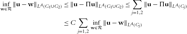
for every u∈LA(G)![]() . The conclusion (2.3.135) follows from (2.3.137) and (2.3.134) applied with G=Gj
. The conclusion (2.3.135) follows from (2.3.137) and (2.3.134) applied with G=Gj![]() , for j=1,2
, for j=1,2![]() .
.
Step 3: The general cases.
Any open Lipschitz domain G is the finite union of open sets Gi![]() , i=1,…,k
, i=1,…,k![]() , starshaped with respect to a ball. Since G is connected, after, possibly, relabelling, we may assume that the sets ∪j−1i=1Gi
, starshaped with respect to a ball. Since G is connected, after, possibly, relabelling, we may assume that the sets ∪j−1i=1Gi![]() and Gj
and Gj![]() have a non-empty intersection. The conclusion then follows from repeated use of (2.3.135). □
have a non-empty intersection. The conclusion then follows from repeated use of (2.3.135). □
Remark 2.3.7
A proof of Corollary 2.3.1 can also be given based on the representation formula (2.3.123). After differentiating (2.3.123) the main part is a singular operator. It can be shown that it enjoys the properties (2.1.34)–(2.1.39). Hence it is continuous from LA(G)![]() to LB(G)
to LB(G)![]() thanks to Theorem 2.1.9. We refer to [31] and [46] for details.
thanks to Theorem 2.1.9. We refer to [31] and [46] for details.
In the following we are concerned with the necessity of the conditions (2.3.107) and (2.3.108) for a Korn-type inequality.
Theorem 2.3.14
Our proof of inequality (2.3.107) is based on the technique of laminates as in [52]. In general a first order laminate is a probability measure ν on Rd×d![]() given by
given by
ν=λδA+(1−λ)δB
where λ∈(0,1)![]() and A,B∈Rd×d
and A,B∈Rd×d![]() with rank(A−B)=1
with rank(A−B)=1![]() . Here δX
. Here δX![]() denotes the Dirac measure concentrated on the matrix X. We say ν has average C if λA+(1−λ)B=C
denotes the Dirac measure concentrated on the matrix X. We say ν has average C if λA+(1−λ)B=C![]() . We obtain a second order laminate if we replace δA
. We obtain a second order laminate if we replace δA![]() (resp. δB
(resp. δB![]() ) by a first order laminate with average A (resp. B). Iteratively we can define laminates of arbitrary order with a given average. For a detailed discussion we refer to [102] and [118].
) by a first order laminate with average A (resp. B). Iteratively we can define laminates of arbitrary order with a given average. For a detailed discussion we refer to [102] and [118].
Lemma 2.3.1
[52], eq. (5)

Proof of Theorem 2.3.14
Part 1: Inequality (2.3.108) holds.
Assume, without loss of generality, that the unit ball B1![]() , centered at 0, is contained in G, and denote by ωd
, centered at 0, is contained in G, and denote by ωd![]() its Lebesgue measure. Let us preliminarily observe that inequality (2.3.138) implies that
its Lebesgue measure. Let us preliminarily observe that inequality (2.3.138) implies that
A dominates B near infinity.
Indeed, given any nonnegative function h∈LA(0,ωd)![]() , consider the function v:B1→Rd
, consider the function v:B1→Rd![]() given by
given by
v(x)=(∫1|x|h(ωdrd)dr,0,…,0)forx∈B1.
Then v∈LA(B1)![]() , and
, and
|ε(v)(x)|⩽|∇v(x)|=h(ωd|x|d)forx∈B1.
An application of (2.3.138), with u replaced by v, shows that
‖h‖LB(0,ωd)=‖∇v‖LB(Ω)⩽C‖ε(v)‖LA(Ω)⩽C‖∇v‖LA(Ω)=‖h‖LA(0,ωd).
Thus LA(0,ωd)→LB(0,ωd)![]() , and (2.3.140) follows.
, and (2.3.140) follows.
Now, given h as above, define the function ρ:[0,1]→[0,∞]![]() by
by
ρ(r)=∫1rh(ωdtd)tdtforr∈[0,1],

and the function v:B1→Rd![]() by
by
u(x)=Qxρ(|x|)forx∈B1,
where Q∈Rd×d![]() is any skew-symmetric matrix such that |Q|=1
is any skew-symmetric matrix such that |Q|=1![]() . We have that u is a weakly differentiable function, and
. We have that u is a weakly differentiable function, and
ε(u)(x)=Qx⊙x|x|2ρ′(|x|)|x|,∇u(x)=Qρ(|x|)+Qx⊗x|x|2ρ′(|x|)|x|

for a.e. x∈B1![]() . Here, ⊙ denotes the symmetric part of the tensor product of two vectors in Rd
. Here, ⊙ denotes the symmetric part of the tensor product of two vectors in Rd![]() . Hence,
. Hence,
|ε(u)(x)|⩽|ρ′(|x|)||x|=h(ωd|x|),ρ(|x|)⩽|∇u(x)|+|ρ′(|x|)||x|=|∇u(x)|+h(ωd|x|)

for a.e. x∈B1![]() . Thus, due to (2.3.138) and (2.3.140),
. Thus, due to (2.3.138) and (2.3.140),
‖∫ωdsh(r)rdr‖LB(0,ωd)=‖∫1|x|h(ωdtd)tdt‖LB(B1)=‖ρ(|x|)‖LB(B1)⩽‖∇u‖LB(B1)+‖h(ωd|x|d)‖LB(B1)⩽C‖ε(u)‖LA(B1)+‖h(ωd|x|d)‖LA(B1)⩽C′‖h(ωd|x|d)‖LA(B1)=C′‖h(s)‖LA(0,ωd)

for suitable constants C and C′![]() . Thanks to the arbitrariness of h, inequality (2.3.141) implies, via Lemma 1.2.1, that (5.3.12) holds for some c and t0
. Thanks to the arbitrariness of h, inequality (2.3.141) implies, via Lemma 1.2.1, that (5.3.12) holds for some c and t0![]() .
.
Part 2: Inequality (2.3.107) holds.
Let us preliminarily note that, if A(t)=∞![]() for large t, then (2.3.107) holds trivially. We may thus assume that A is finite-valued, and hence continuous. By (2.3.140), the function B is also finite-valued and continuous.
for large t, then (2.3.107) holds trivially. We may thus assume that A is finite-valued, and hence continuous. By (2.3.140), the function B is also finite-valued and continuous.
For ease of notations, we hereafter focus on case when d=2![]() . An analogous argument carries over to any dimension along the lines of [52, Lemma 3]. Given a,b∈R
. An analogous argument carries over to any dimension along the lines of [52, Lemma 3]. Given a,b∈R![]() , we define the matrix Ga,b
, we define the matrix Ga,b![]() as
as
Ga,b=(0ab0),

and set δa,b=δGa,b![]() . Next, we define the sequence {μ(m)}
. Next, we define the sequence {μ(m)}![]() of laminates of order 2m iteratively by
of laminates of order 2m iteratively by
{μ(0)=δt,t,μ(m)=13δ2−mt,−2−mt+16δ−21−mt,21−mt+12μ(m−1)

for m∈N![]() . We claim that μ(m)
. We claim that μ(m)![]() is a laminate with average G2−mt,2−mt
is a laminate with average G2−mt,2−mt![]() for m∈N
for m∈N![]() . Indeed, the following holds
. Indeed, the following holds
μ(m)=14δ−21−mt,21−mt+34μ(m−1).
Since rank(G−t,t−Gt,t)=1![]() , the right-hand side of (2.3.143) is a laminate with average G2−1t,t
, the right-hand side of (2.3.143) is a laminate with average G2−1t,t![]() for m=1
for m=1![]() . Hence, μ(1)
. Hence, μ(1)![]() is a laminate with average G2−1t,2−1t
is a laminate with average G2−1t,2−1t![]() . An induction argument then proves our claim. Now, note the representation formula
. An induction argument then proves our claim. Now, note the representation formula
μ(m)=2−mδt,t+m∑k=1(132k−mδ2−kt,−2−kt+162k−mδ−21−kt,21−kt)

for m∈N![]() . We remark that δt,t
. We remark that δt,t![]() is concentrated at a symmetric matrix, whereas the sum in (2.3.144) is concentrated at skew-symmetric matrices. We define the functions Φj:R2×2→[0,∞)
is concentrated at a symmetric matrix, whereas the sum in (2.3.144) is concentrated at skew-symmetric matrices. We define the functions Φj:R2×2→[0,∞)![]() , for j=1,2
, for j=1,2![]() , by
, by
Φ1(X)=A(|Xsym−G2−mt,2−mt|),Φ2(X)=B(C−1|X−G2−mt,2−mt|),

for X∈R2×2![]() . Here, Xsym=12(X+XT)
. Here, Xsym=12(X+XT)![]() is the symmetric part of X, and C is the constant appearing in (2.3.138). Fix m∈N
is the symmetric part of X, and C is the constant appearing in (2.3.138). Fix m∈N![]() . Without loss of generality, we may assume that 0∈G
. Without loss of generality, we may assume that 0∈G![]() . We choose r>0
. We choose r>0![]() so small that (0,r)2⊂G
so small that (0,r)2⊂G![]() . Let m∈N
. Let m∈N![]() be arbitrary. Due to Lemma 2.3.1 applied with ν=μ(m)
be arbitrary. Due to Lemma 2.3.1 applied with ν=μ(m)![]() , there exists a sequence {ui}
, there exists a sequence {ui}![]() of Lipschitz continuous functions ui:(0,r)2→R2
of Lipschitz continuous functions ui:(0,r)2→R2![]() , such that ui(x)=G2−mt,2−mtx
, such that ui(x)=G2−mt,2−mtx![]() on ∂(0,r)2
on ∂(0,r)2![]() , and
, and
limi→∞∫(0,r)2Φj(∇ui)dx=r2∫R2×2Φj(X)dμ(m)(X)forj=1,2.

We define the sequence {vi}![]() of functions vi:G→R
of functions vi:G→R![]() by vi(x)=ui(x)−G2−mt,2−mtx
by vi(x)=ui(x)−G2−mt,2−mtx![]() if x∈(0,r)2
if x∈(0,r)2![]() , and vi(x)=0
, and vi(x)=0![]() if G∖(0,r)2
if G∖(0,r)2![]() . Then vi∈W1,∞0(G)
. Then vi∈W1,∞0(G)![]() , and, by (2.3.145),
, and, by (2.3.145),
limi→∞∫GA(|ε(vi)|)dx=limi→∞∫(0,r)2A(|ε(v)i|)dx

=r2∫R2×2A(|(Xsym−G2−mt,2−mt)|)dμ(m)(X),limi→∞∫ΩB(C−1|∇vi|)dx=limi→∞∫(0,r)2B(C−1|∇vi|)dx=r2∫R2×2B(C−1|X−G2−mt,2−mt|)dμ(m)(X).

We have the following chain
∫R2×2A(|Xsym−G2−mt,2−mt|)dμ(m)(X)⩽12∫R2×2A(2|Xsym|)dμ(m)(X)+12∫R2×2A(2|G2−mt,2−mt|)dμ(m)(X)=122−mA(2|Gt,t|)+12A(2|G2−mt,2−mt|)=122−mA(2|Gt,t|)+12A(22−m|Gt,t|)⩽2−mA(2|Gt,t|).

Here the first inequality holds since A is convex, the first equality holds due to (2.3.144) and to the fact that μ(m)![]() is a probability measure, and the last inequality follows from (1.2.6). Combining (2.3.146) with (2.3.148) implies
is a probability measure, and the last inequality follows from (1.2.6). Combining (2.3.146) with (2.3.148) implies
limi→∞∫GA(|ε(vi)|)dx⩽r22−mA(2|Gt,t|).

Since A is a continuous function, there exists tm∈(0,∞)![]() such that
such that
r22−mA(2|Gtm,tm|)=12.
Thanks to (1.2.6), there exists t0>0![]() , independent of m, such that
, independent of m, such that
tm⩽t02m.
Therefore, by neglecting, if necessary, a finite number of terms of the sequence {vi}![]() , we can assume that
, we can assume that
∫GA(|ε(vi)|)dx⩽1

for i∈N![]() . Hence, ‖ε(vi)‖A⩽1
. Hence, ‖ε(vi)‖A⩽1![]() for i∈N
for i∈N![]() , and, by (2.3.138), ‖∇vi‖B⩽C
, and, by (2.3.138), ‖∇vi‖B⩽C![]() for i∈N
for i∈N![]() . Thus,
. Thus,
∫GB(C−1|∇vi|)dx⩽1

for i∈N![]() . Combining the latter inequality with equation (2.3.147) implies us that
. Combining the latter inequality with equation (2.3.147) implies us that
r2∫R2×2B(C−1|X−G2−mtm,2−mtm|)dμ(m)(X)⩽1.

Next, one can make use of (2.3.144) and obtain the following chain
r−2⩾∫R2×2B(C−1|X−G2−mtm,2−mtm|)dμ(m)(X)⩾2−mB(C−1(1−2−m)|Gtm,tm|)+m∑k=1132k−mB(C−1(2−k−2−m)|Gtm,tm|)+m∑k=1162k−mB(C−1(21−k−2−m)|Gtm,tm|)⩾m−1∑k=1132k−mB(C−1(2−k−2−m)|Gtm,tm|)⩾m−1∑k=1132k−mB(C−12−k−1|Gtm,tm|)⩾m−1∑k=11312C2−mtmB(12C2−ktm)12C2−ktm.

It follows from (2.3.150), (2.3.152) and (2.3.153) that
2⋅2−mA(2|Gtm,tm|)⩾m−1∑k=11312C2−mtmB(12C2−ktm)12C2−ktm.

Hence, by (2.3.151),
A(c″tm)⩾ctmm−1∑k=1B(12C2−ktm)12C2−ktm⩾c′tm∫tm4C2−mtm4CB(s)s2ds⩾c′tm∫tm4Ct02CB(s)s2ds

for suitable positive constants c, c′![]() c″
c″![]() . Since limm→∞tm=∞
. Since limm→∞tm=∞![]() , one can find ˆt⩾t02C
, one can find ˆt⩾t02C![]() such that, if t>ˆt
such that, if t>ˆt![]() , then there exists m∈N
, then there exists m∈N![]() such that tm⩽t<tm+1
such that tm⩽t<tm+1![]() . Moreover, ˆt
. Moreover, ˆt![]() can be chosen so large that A is invertible on [ˆt,∞)
can be chosen so large that A is invertible on [ˆt,∞)![]() and
and
tm=c1A−1(c22m)
for some positive constants c1,c2![]() . By (1.2.7), the latter equation ensures that tm+1⩽2tm
. By (1.2.7), the latter equation ensures that tm+1⩽2tm![]() for m∈N
for m∈N![]() . Thus, due to inequality (2.3.154),
. Thus, due to inequality (2.3.154),
A(2c″t)⩾A(2c″tm)⩾A(c″tm+1)⩾c′tm+1∫tm+14Ct02CB(s)s2ds⩾c′t∫t4Ct02CB(s)s2ds

for t⩾ˆt![]() . Hence, inequality (2.3.107) follows for suitable constants c and t0
. Hence, inequality (2.3.107) follows for suitable constants c and t0![]() . □
. □
Corollary 2.3.2
Proof
Let u∈W1,A0(G)![]() . As in the proof of Theorem (2.3.119) we can show the following chain
. As in the proof of Theorem (2.3.119) we can show the following chain
‖∇u−(∇u)G‖LB(G)=‖∇u−(∇u)G‖LB(G)⩽Cd∑i,j=1‖∂ui∂xj−(∂ui∂xj)G‖LB(G)⩽Cn∑i,j=1‖∇∂ui∂xj‖W−1,A(G)⩽Cd∑i,j,k=1‖∂2ui∂xk∂xj‖W−1,A(G)⩽Cd∑i,j,k=1(‖∂(ε(u))ij∂xk‖W−1,A(G)+‖∂(ε(u))ik∂xj‖W−1,A(G)+‖∂(ε(u))jk∂xi‖W−1,A(G))⩽Cd∑i,j=1‖∇(ε(u))ij‖W−1,A(G)⩽Cn∑i,j=1‖(ε(u))ij−((ε(u))ij)G‖LA(G)⩽C‖ε(u)−(ε(u))G‖LA(G)=C‖ε(u)‖LA(G).

Here the second inequality in line two holds by (2.3.155). The first inequality in line four is true for every Young function by the very definition of the negative norm. The conclusion follows via Theorem 2.3.14, due to the arbitrariness of u. □
Corollary 2.3.3
Let G be a bounded domain in Rd![]() , d⩾2
, d⩾2![]() , which is starshaped with respect to a ball, and let BogG
, which is starshaped with respect to a ball, and let BogG![]() be the Bogovskiĭ operator on G (see Section 2.1). Let A and B be Young functions such that
be the Bogovskiĭ operator on G (see Section 2.1). Let A and B be Young functions such that
‖∇BogGf‖LB(G,Rd)⩽C‖f‖LA(G)
for some constant C, and for every f∈C∞0,⊥(G)![]() . Then conditions (2.0.11) and (2.0.12) hold.
. Then conditions (2.0.11) and (2.0.12) hold.