
Solenoidal Lipschitz truncation
Abstract
In this chapter we present the solenoidal Lipschitz truncation for non-stationary problems: we show how to construct a Lipschitz truncation which preserves the divergence-free character of a given Sobolev function. As a matter of fact, it suffices to have distributional time-derivatives in the sense of divergence-free test-functions. After this, we present the A![]() -Stokes approximation for non-stationary problems. It aims at approximating almost solutions to the non-stationary A
-Stokes approximation for non-stationary problems. It aims at approximating almost solutions to the non-stationary A![]() -Stokes system by exact solutions. Thanks to the solenoidal Lipschitz truncation this can be done on the level of gradients.
-Stokes system by exact solutions. Thanks to the solenoidal Lipschitz truncation this can be done on the level of gradients.
Keywords
Solenoidal Lipschitz truncation; Divergence-free constraint; Parabolic PDEs; Inverse curl-operator; A![]() -Stokes approximation; Almost solutions
-Stokes approximation; Almost solutions
In this chapter we develop a non-stationary counterpart of the solenoidal Lipschitz truncation from Chapter 3. Here, the main difficulty is to handle problems connected with the distributional time derivative of the function we aim to truncate. Let us be a little bit more precise. Let Q0=I0×B0⊂R×R3![]() be a space time cylinder and σ∈(1,∞)
be a space time cylinder and σ∈(1,∞)![]() . Let u∈Lσ(I0,W1,σdiv(B0))
. Let u∈Lσ(I0,W1,σdiv(B0))![]() and G∈Lσ(Q0)
and G∈Lσ(Q0)![]() satisfy
satisfy
∫Q0∂tu⋅ξdxdt=∫Q0G:∇ξdxdtfor allξ∈C∞0,div(Q0).

The main purpose of the solenoidal Lipschitz truncation is to avoid the appearance of the pressure function. Hence we start in (6.0.1) with an equation on the level of divergence-free test-functions. Unfortunately, this is not enough information on the time derivative for a Poincaré-type inequality as in (5.2.6). Hence the approach from [65] as explained in Section 5.2 will not give L∞![]() -estimates for the gradient of the truncation, cf. the proof of Lemma 5.2.3. Our aim is to construct a truncation which preserves the properties from [65] and is, in addition, divergence-free.
-estimates for the gradient of the truncation, cf. the proof of Lemma 5.2.3. Our aim is to construct a truncation which preserves the properties from [65] and is, in addition, divergence-free.
We will show that there is a truncation uλ![]() of u with roughly the following properties (see Theorem 6.1.25 for a precise formulation).
of u with roughly the following properties (see Theorem 6.1.25 for a precise formulation).
(a) ∇uλ∈L∞(Q0)![]() with ‖∇uλ‖∞⩽cλ
with ‖∇uλ‖∞⩽cλ![]() and divuλ=0
and divuλ=0![]() .
.
(b) uλ=u![]() a.e. outside a suitable set Oλ
a.e. outside a suitable set Oλ![]() .
.
(c) There holds
|〈∂tu,uλ−u〉|+‖χOαλ∇uλ‖pp⩽cλp|Oλ|⩽δ(λ),
with δ(λ)→0![]() if λ→∞
if λ→∞![]() .
.
In the following we sketch the construction on a heuristic level. In fact, the rigorous approach which we shall present in the next section requires a series of localization arguments, so it is quite technical. Let us start with a function
u∈L∞(I0;L2(B0))∩Lp(I0;W1,p0,div(B0))
with ∂tu=divH![]() in D′div(B0)
in D′div(B0)![]() , where H∈Lσ(B)
, where H∈Lσ(B)![]() for some σ>1
for some σ>1![]() . We define
. We define
w:=curl−1u∈L∞(I0;W1,2(B0))∩Lp(I0;W2,pdiv(B0)).
It follows that ∂tΔw=curldivH![]() in D′(B0)
in D′(B0)![]() . Also we can obtain an information about the time derivative of w as a distribution acting on all test-functions. However, we do not have control about a possible harmonic part of w. Hence we decompose w into a harmonic and anti-harmonic part. To do this we define, pointwise in time,
. Also we can obtain an information about the time derivative of w as a distribution acting on all test-functions. However, we do not have control about a possible harmonic part of w. Hence we decompose w into a harmonic and anti-harmonic part. To do this we define, pointwise in time,
w(t)=z(t)+h(t),
where z(t)∈ΔW2,p0(B0)![]() and Δh(t)=0
and Δh(t)=0![]() . This decomposition is based on a singular integral operator which is continuous on Lp
. This decomposition is based on a singular integral operator which is continuous on Lp![]() -spaces such that
-spaces such that
z,w∈L∞(I0;W1,2(B0))∩Lp(I0;W2,p(B0)).
Moreover, we have
∂tΔz=∂tw=curldivH
in D′(B0)![]() . As z is anti-harmonic by construction this yields
. As z is anti-harmonic by construction this yields
‖∂tz‖σ⩽c‖H‖σ.
In fact, ∂tz![]() is a measurable function. Now, we truncate z to zλ
is a measurable function. Now, we truncate z to zλ![]() with an approach similar to (5.2.8). This truncation satisfies with ‖∇2zλ‖∞⩽cλ
with an approach similar to (5.2.8). This truncation satisfies with ‖∇2zλ‖∞⩽cλ![]() as well as zλ=z
as well as zλ=z![]() in Oλ
in Oλ![]() , where Oλ=Oλ(M(∇2z);M(∂tz))
, where Oλ=Oλ(M(∇2z);M(∂tz))![]() . Finally, we set
. Finally, we set
uλ:=curlzλ+curlh.
Obviously, we have divuλ=0![]() . Due to (6.0.2) and the properties of harmonic functions we have h∈L∞(I0;Wk,2(B0))
. Due to (6.0.2) and the properties of harmonic functions we have h∈L∞(I0;Wk,2(B0))![]() for any k∈N
for any k∈N![]() (at least locally in space). Hence uλ
(at least locally in space). Hence uλ![]() has the same regularity as curlzλ
has the same regularity as curlzλ![]() . In particular, ∇uλ
. In particular, ∇uλ![]() is bounded.
is bounded.
In Section 6.2 we develop the A![]() -Stokes approximation for non-stationary problems, see [29]. This is, on the one hand, a non-stationary variant of the A
-Stokes approximation for non-stationary problems, see [29]. This is, on the one hand, a non-stationary variant of the A![]() -Stokes approximation from Section 3.3. On the other hand it is a fluid-mechanical counterpart of the A
-Stokes approximation from Section 3.3. On the other hand it is a fluid-mechanical counterpart of the A![]() -caloric approximation from [68] which is concerned with the A
-caloric approximation from [68] which is concerned with the A![]() -heat equation.
-heat equation.
6.1 Solenoidal truncation – evolutionary case
In this section we examine solenoidal functions, whose time derivative is only a distribution acting on solenoidal test-functions. Let u∈Lσ(I0,W1,σdiv(B0))![]() be such that (6.0.1) holds for some G∈Lσ(Q0)
be such that (6.0.1) holds for some G∈Lσ(Q0)![]() . So the time derivative is only well defined via the duality with solenoidal test functions. The goal of this section is to construct a solenoidal truncation uλ
. So the time derivative is only well defined via the duality with solenoidal test functions. The goal of this section is to construct a solenoidal truncation uλ![]() of u which preserves the properties of the truncation in [65].
of u which preserves the properties of the truncation in [65].
First we extend our function u in a suitable way to the whole space and then apply the inverse curl operator. Let γ∈C∞0(B0)![]() with χ12B0⩽γ⩽χB0
with χ12B0⩽γ⩽χB0![]() , where B0
, where B0![]() is a ball. Let C0
is a ball. Let C0![]() denote the annulus B0∖12B0
denote the annulus B0∖12B0![]() . Then according to Theorem 2.1.6 (with A(t)=B(t)=tq
. Then according to Theorem 2.1.6 (with A(t)=B(t)=tq![]() ) there exists a Bogovskiĭ operator BogC0:C∞0,⊥(C0)→C∞0(C0)
) there exists a Bogovskiĭ operator BogC0:C∞0,⊥(C0)→C∞0(C0)![]() which is bounded from Lq⊥(C0)→W1,q0(C0)
which is bounded from Lq⊥(C0)→W1,q0(C0)![]() for all q∈(1,∞)
for all q∈(1,∞)![]() , and such that divBogC0=Id
, and such that divBogC0=Id![]() . Define
. Define
˜u:=γu−BogC0(div(γu))=γu−BogC0(∇γ⋅u).
Then div˜u=0![]() on I0×B0
on I0×B0![]() and ˜u(t)∈W1,σ0(B0)
and ˜u(t)∈W1,σ0(B0)![]() , so we can extend ˜u
, so we can extend ˜u![]() by zero in space to ˜u∈Lσ(I0,W1,σdiv(R3))
by zero in space to ˜u∈Lσ(I0,W1,σdiv(R3))![]() . Since ˜u=u
. Since ˜u=u![]() on I0×12B0
on I0×12B0![]() , we have
, we have
∫Q0∂t˜u⋅ξdxdt=∫Q0G:∇ξdxdtfor allξ∈C∞0,div(12Q0).

Now, we define, pointwise in time,
w:=curl−1(˜u)=curl−1(γu−BogC0(∇γ⋅u)).
Overall, we get the following lemma.
Lemma 6.1.1


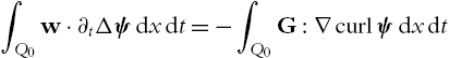
Let us derive from (6.0.1) the equation for w. For ψ∈C∞0(12Q0)![]() we have
we have
∫Q0∂tu⋅curlψdxdt=∫Q0G:∇curlψdxdt.

We use u=curlw![]() and partial integration to show that
and partial integration to show that
∫Q0∂tw⋅curlcurlψdxdt=∫Q0G:∇curlψdxdt.

Now, because
∫Q0w⋅∂t∇divψdxdt=∫Q0divw∂tdivψdxdt=0

and curlcurlψ=−Δψ+∇divψ![]() we obtain
we obtain
∫Q0w⋅∂tΔψdxdt=−∫Q0G:∇curlψdxdt
for every ψ∈C∞0(12Q0)![]() . We can rewrite this as
. We can rewrite this as
∫Q0w⋅∂tΔψdxdt=−∫Q0H:∇2ψdxdt,

with |G|∼|H|![]() pointwise. In particular, in the sense of distributions we have
pointwise. In particular, in the sense of distributions we have
∂tΔw=−curldivG=−divdivH.
So in passing from u to w we got a system valid for all test functions ψ∈C∞0(Q0)![]() . However, we only have control of ∂tΔw
. However, we only have control of ∂tΔw![]() , so that the time derivative of the harmonic part of w cannot be seen. Hence, a parabolic Poincaré inequality for w still does not hold; i.e. ∂tw
, so that the time derivative of the harmonic part of w cannot be seen. Hence, a parabolic Poincaré inequality for w still does not hold; i.e. ∂tw![]() is not controlled! In order to remove this harmonic invariance we will replace w by some function z such that ∂tΔw=∂tΔz
is not controlled! In order to remove this harmonic invariance we will replace w by some function z such that ∂tΔw=∂tΔz![]() . This will imply that ∂tz
. This will imply that ∂tz![]() can be controlled by H. To define z conveniently we need some auxiliary results.
can be controlled by H. To define z conveniently we need some auxiliary results.
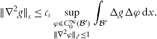
For a ball B′⊂R3![]() and a function f∈Ls(B′)
and a function f∈Ls(B′)![]() we define Δ−2B′Δf
we define Δ−2B′Δf![]() as the weak solution F∈W2,s0(B′)
as the weak solution F∈W2,s0(B′)![]() of
of
∫B′ΔFΔφdx=∫B′fΔφdxfor allφ∈C∞0(B′).

Then f−Δ(Δ−2B′Δf)![]() is harmonic on B′
is harmonic on B′![]() .
.
According to [117] and Lemma 2.1 of [140] we have the following variational estimate.
This implies the following two corollaries.
Corollary 6.1.1

Proof

Corollary 6.1.2

For V∈Ls(B′)![]() we define Δ−2B′divdivV
we define Δ−2B′divdivV![]() as the weak solution F∈W2,s0(B′)
as the weak solution F∈W2,s0(B′)![]() of
of
∫B′ΔFΔφdx=∫B′V∇2φdxfor allφ∈C∞0(B′).

Similar to Corollary 6.1.1 we get the following result.
Corollary 6.1.3

The next lemma shows the wanted control of the time derivative.
Lemma 6.1.3

Proof
The estimate of zQ′![]() in terms of w follows directly from Corollary 6.1.1 and integration over time. The estimate of zQ′
in terms of w follows directly from Corollary 6.1.1 and integration over time. The estimate of zQ′![]() in terms of ∇w
in terms of ∇w![]() and ∇2w
and ∇2w![]() follows from this by Poincaré's inequality, using the fact that we can subtract a linear polynomial from w without changing the definition of zQ′
follows from this by Poincaré's inequality, using the fact that we can subtract a linear polynomial from w without changing the definition of zQ′![]() . The other estimate for ∇zQ′
. The other estimate for ∇zQ′![]() and ∇2zQ′
and ∇2zQ′![]() follow analogously from Corollary 6.1.2.
follow analogously from Corollary 6.1.2.
For all ρ∈C∞0(I′)![]() and φ∈C∞0(B′)
and φ∈C∞0(B′)![]() it follows from (6.1.5) that
it follows from (6.1.5) that
∫I′∫B′w⋅Δφdx∂tρdt=−∫I′∫B′H:∇2φdxρdt.

Let dht![]() denote the forward difference quotient in time with step size h. We use ρ(t):=⨍t−ht˜ρ(τ)dτ
denote the forward difference quotient in time with step size h. We use ρ(t):=⨍t−ht˜ρ(τ)dτ![]() with ˜ρ∈C∞0(I′)
with ˜ρ∈C∞0(I′)![]() and h sufficiently small. Then ∂tρ=d−ht˜ρ
and h sufficiently small. Then ∂tρ=d−ht˜ρ![]() and
and
∫I′∫B′w⋅Δφdxd−ht˜ρdt=−∫I′∫B′H:∇2φdx⨍t−ht˜ρ(τ)dτdt.

This implies that
∫I′∫B′dhtw⋅Δφdx˜ρdt=−∫I′∫B′⨍t+htH(τ)dτ:∇2φdx˜ρdt.

Since this is valid for all choices of ˜ρ![]() we have
we have
∫B′dhtw⋅Δφdx=−∫B′⨍t+htH(τ)dτ:∇2φdx.

Since dhtzQ′=dht(ΔΔ−2B′Δw)=ΔΔ−2B′Δ(dhtw)![]() , it follows by Corollary 6.1.1 that
, it follows by Corollary 6.1.1 that
(∫B′|dhtzQ′|sdx)1s⩽csupφ∈C∞0(B)‖∇2φ‖s′⩽1∫B′dhtwΔφdx=supφ∈C∞0(B)‖∇2φ‖s′⩽1(−∫B′⨍t+htH(τ)dτ:∇2φdx)⩽c(∫B′⨍t+ht|H(τ)|sdτdx)1s.

Integrating over time and passing to the limit h→0![]() yields
yields
(∫Q′|∂tzQ′|sdxdt)1s⩽c(∫Q′|H|sdxdt)1s

which finishes the proof. □
Defining z(t):=z12Q0(t)=ΔΔ−212B0Δw(t)![]() for t∈12I0
for t∈12I0![]() , we then have
, we then have
∫Q0z⋅∂tΔψdxdt=∫Q0w⋅∂tΔψdxdt=−∫Q0H:∇2ψdxdt,

for all ψ∈C∞0(12Q0)![]() . Since the function Δ−212B0w(t)∈W2,s0(12B0)
. Since the function Δ−212B0w(t)∈W2,s0(12B0)![]() , we can extend it by zero to a function in W2,s(R3)
, we can extend it by zero to a function in W2,s(R3)![]() . In this sense it is natural to extend z(t)
. In this sense it is natural to extend z(t)![]() by zero to a function in Ls(R3)
by zero to a function in Ls(R3)![]() .
.
Note that Lemma 6.1.3 enables us to control ∂tz![]() by H in Ls(12Q0)
by H in Ls(12Q0)![]() .
.
Lemma 6.1.4

For λ,α>0![]() and σ>1
and σ>1![]() we define
we define
Oαλ:={Mασ(χ13Q0|∇2z|)>λ}∪{αMασ(χ13Q0|∂tz|)>λ}.
Later we will choose α=λ2−p![]() and σ smaller than the integrability exponent of ∂tz
and σ smaller than the integrability exponent of ∂tz![]() . We want to redefine z on Oαλ
. We want to redefine z on Oαλ![]() . The first step is to cover Oαλ
. The first step is to cover Oαλ![]() by well selected cubes. By the lower-semi-continuity property of the maximal functions the set Oαλ
by well selected cubes. By the lower-semi-continuity property of the maximal functions the set Oαλ![]() is open. We assume in the following that Oαλ
is open. We assume in the following that Oαλ![]() is non-empty. (In the case that Oαλ
is non-empty. (In the case that Oαλ![]() is empty, we do not need to truncate at all.) We cover Oαλ
is empty, we do not need to truncate at all.) We cover Oαλ![]() by an α-parabolic Whitney covering {Qi}
by an α-parabolic Whitney covering {Qi}![]() with partition of unity in accordance with Lemmas 5.2.1 and 5.2.2.
with partition of unity in accordance with Lemmas 5.2.1 and 5.2.2.
Due to property (PW3) we have that 16Qj∩(Rd+1∖Oαλ)≠∅![]() . Thus, the definition of Oαλ
. Thus, the definition of Oαλ![]() implies that
implies that
(⨍16Qj|∇2z|σχ13Q0dxdt)1σ⩽λ,

α(⨍16Qj|∂tz|σχ13Q0dxdt)1σ⩽λ.

Lemma 6.1.5
Assume that there exists c0>0![]() such that λp|Oαλ|⩽c0
such that λp|Oαλ|⩽c0![]() with p>2dd+2
with p>2dd+2![]() . Then the following holds:
. Then the following holds:
if λ⩾λ0=λ0(c0)![]() , α=λ2−p
, α=λ2−p![]() and Qi∩14Q0≠∅
and Qi∩14Q0≠∅![]() , then Qi⊂13Q0
, then Qi⊂13Q0![]() and Qj⊂13Q0
and Qj⊂13Q0![]() for all j∈Ai
for all j∈Ai![]() .
.
Proof
Let Qi∩14Q0≠∅![]() . We claim that Qi⊂724Q0⊂13Q0
. We claim that Qi⊂724Q0⊂13Q0![]() . Let si:=αr2i
. Let si:=αr2i![]() . It suffices to show that ri,si→0
. It suffices to show that ri,si→0![]() as λ→∞
as λ→∞![]() . Because Qi⊂Oαλ
. Because Qi⊂Oαλ![]() and by assumption, we find
and by assumption, we find
λ2rd+2i=λpsirdi⩽cλp|Qi|⩽cλp|Oαλ|⩽cc0.
This implies that ri⩽(cc0λ−2)1d+2→0![]() as λ→∞
as λ→∞![]() . Moreover, ri=s12iα−12
. Moreover, ri=s12iα−12![]() and (6.1.11) imply
and (6.1.11) imply
cc0⩾λpsirdi=λpsd+22iα−32=λd+22p−dsd+22i.
If p>2dd+2![]() , then λ→∞
, then λ→∞![]() implies si→0
implies si→0![]() as desired.
as desired.
The claim on j∈Ai![]() follows from the fact that Qi
follows from the fact that Qi![]() and Qj
and Qj![]() have comparable size and that 724Q0
have comparable size and that 724Q0![]() is strictly contained in 13Q0
is strictly contained in 13Q0![]() . □
. □
Let us show that the assumption λp|Oαλ|⩽c0![]() from Lemma 6.1.5 is satisfied in our situation. To do this we assume from now on that
from Lemma 6.1.5 is satisfied in our situation. To do this we assume from now on that
α:=λ2−p
and that σ<min{p,p′}![]() .
.
Proof
It follows from the weak-type estimate of Mασ![]() in (5.2.5), if σ<min{p,p′}
in (5.2.5), if σ<min{p,p′}![]() , then
, then
|Oαλ|⩽cλ−p‖∇2z‖pLp(13Q0)+c(λα−1)−p′‖∂tz‖p′Lp′(13Q0)=cλ−p(‖∇2z‖pLp(13Q0)+‖∂tz‖p′Lp′(13Q0)).

□
In the following we choose λ0![]() such that the conclusion of Lemma 6.1.5 is valid and assume λ⩾λ0
such that the conclusion of Lemma 6.1.5 is valid and assume λ⩾λ0![]() . Without loss of generality we can assume further that
. Without loss of generality we can assume further that
λ0⩾(⨍13Q0|∇2z|σdxdt)1σ+r−20(⨍13Q0|z|σdxdt)1σ.

We define
I:={i:Qi∩14Q0≠∅}.
Then Lemma 6.1.5 implies that Qi⊂13Q0![]() (and Qj⊂13Q0
(and Qj⊂13Q0![]() for j∈Ai
for j∈Ai![]() ) for all i∈I
) for all i∈I![]() . For each i∈I
. For each i∈I![]() we define local approximation zi
we define local approximation zi![]() for z on Qi
for z on Qi![]() by
by
zi:=Π0IiΠ1Bi(z),
where Π1Bi(z)![]() is the first order averaged Taylor polynomial [37,63] with respect to space and Π0Ii
is the first order averaged Taylor polynomial [37,63] with respect to space and Π0Ii![]() is the zero order averaged Taylor polynomial in time. Note that this definition implies the Poincaré-type inequality.
is the zero order averaged Taylor polynomial in time. Note that this definition implies the Poincaré-type inequality.
Lemma 6.1.7

Proof
The estimate is a consequence of Fubini's Theorem, Poincaré estimates and the properties of the averaged Taylor polynomials see Lemma 3.1 of [63]. We find
⨍Qj|z−zjr2j|sdxdt⩽c⨍Qj|z−Π1Bj(z)r2j|sdxdt+c⨍Bj⨍Ij|Π1Bj(z)−Π0IjΠ1Bj(z)r2j|sdxdt⩽c⨍Qj|∇2z|sdxdt+cα⨍Ij⨍Bj|∂tΠ1Bj(z)|sdxdt.

Now the continuity of Π1Bj![]() on Ls
on Ls![]() gives the estimate. Similarly we find (since all norms for polynomials are equivalent)
gives the estimate. Similarly we find (since all norms for polynomials are equivalent)
⨍Qj|∇(z−zj)rj|sdxdt⩽c⨍Qj|∇(z−Π1Bj(z))rj|sdxdt+c⨍Qj|∇(Π1Bj(z)−Π0IjΠ1Bj(z))rj|sdxdt⩽c⨍Qj|∇(z−Π1Bj(z))rj|sdxdt+c⨍Qj|Π1Bj(z)−Π0IjΠ1Bj(z)r2j|sdxdt⩽c⨍Qj|∇2z|sdxdt+cα⨍Qj|∂tz|sdxdt.

□
We can now define our truncation zαλ![]() for λ⩾λ0
for λ⩾λ0![]() on 14Q0
on 14Q0![]() by
by
zαλ:=z−∑i∈Iφi(z−zi).
It suffices to sum over i with Qi∩14Q0≠∅![]() .
.
Since the φi![]() are locally finite, this sum is pointwise well-defined. We will see later that the sum converges also in other topologies. Using ∑i∈Iφi=1
are locally finite, this sum is pointwise well-defined. We will see later that the sum converges also in other topologies. Using ∑i∈Iφi=1![]() on 14Q0
on 14Q0![]() , we can also write zαλ
, we can also write zαλ![]() in the form
in the form
zαλ={zin14Q0∖Oαλ,∑i∈Iφiziin14Q0∩Oαλ.

In the following we describe some properties of the truncation (e.g. ∇2zαλ∈L∞(14Q0)![]() ).
).
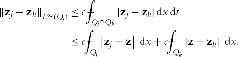
Lemma 6.1.8
For all j∈N![]() and all k∈N
and all k∈N![]() with Qj∩Qk≠∅
with Qj∩Qk≠∅![]() we have
we have
(a) ⨍Qj|∇2z|dxdt+α⨍Qj|∂tz|dxdt⩽cλ![]() .
.
(b) ‖zj−zk‖L∞(Qj)⩽c⨍Qj|z−zj|dxdt+c⨍Qk|z−zk|dxdt![]() .
.
(c) ‖zj−zk‖L∞(Qj)⩽cr2jλ![]() .
.
Proof
Part (a) follows from Qj⊂16Qj![]() and 16Qj∩O∁λ≠∅
and 16Qj∩O∁λ≠∅![]() , so
, so
⨍16Qj(|∇2z|+α|∂tz|)χ13Q0dxdt⩽(⨍16Qj(|∇2z|+α|∂tz|)σχ13Q0dxdt)1σ⩽cλ.

Part (b) follows from the geometric property of the Qj![]() . If Qj∩Qk≠∅
. If Qj∩Qk≠∅![]() , then |Qj∩Qk|⩾cmax{|Qj|,|Qk|}
, then |Qj∩Qk|⩾cmax{|Qj|,|Qk|}![]() . This and the norm equivalence for linear polynomials imply
. This and the norm equivalence for linear polynomials imply
‖zj−zk‖L∞(Qj)⩽c⨍Qj∩Qk|zj−zk|dxdt⩽c⨍Qj|zj−z|dx+c⨍Qk|z−zk|dx.
Finally, (c) is a consequence of Lemma 6.1.7, (a) and (b). □
Next, we prove the stability of the truncation.
Lemma 6.1.9
Let 1<s<∞![]() and z∈Ls(R;W2,s(R3))
and z∈Ls(R;W2,s(R3))![]() . Then
. Then
‖zαλ‖Ls(14Q0)⩽c‖z‖Ls(13Q0),‖∇zαλ‖Ls(14Q0)⩽c‖∇z‖Ls(13Q0)+cαr0‖∂tz‖Ls(13Q0),‖∇2zαλ‖Ls(14Q0)+α‖∂tzαλ‖Ls(13Q0)⩽c‖∇2z‖Ls(13Q0)+cα‖∂tz‖Ls(13Q0).

Moreover, the sum in (6.1.15) converges in Ls(14I0,W2,s(14B0))![]() .
.
Proof
We first show that the sum in (6.1.15) converges absolutely in Ls(14Q0)![]() :
:
∫14Q0|z−zαλ|sdx⩽∑i∈I∫Qi|z−zi|sdxdt⩽c∑i∈I∫Qi|z|sdxdt⩽c∫13Q0|z|sdt,

where we used continuity of the mapping z↦zi![]() in Ls(Qi)
in Ls(Qi)![]() , (PP1) and the finite intersection property of Qi
, (PP1) and the finite intersection property of Qi![]() (PW4). We start by showing the estimate for the second derivatives
(PW4). We start by showing the estimate for the second derivatives
∫Oαλ|∇2(z−zαλ)|sdxdt=|∑i∈I∫Qi∇2(φi(z−zi))dxdt|⩽c∑i∈I∫Qi|∇2z|s+|∇(z−zi)ri|s+|z−zir2i|sdxdt.

For the time derivative we find (since zi![]() is constant in time), that
is constant in time), that
∫Oαλ|∂t(z−zαλ)|sdxdt=|∑i∈I∫Qi∂t(φi(z−zi))dxdt|⩽c∑i∈I∫Qi|∂tz|s+|z−ziαr2i|sdxdt.

Using Lemma 6.1.7 and the finite intersection of the Qi![]() shows that
shows that
∫14Q0|∇2(z−zαλ)|s+αs|∂t(z−zαλ)|sdxdt⩽c∑i∈I∫Qi|∇2z|s+αs|∂tz|sdxdt⩽c∫13Q0|∇2z|s+αs|∂tz|sdxdt.

The estimate of the gradient is analogous, since
∫Oαλ|∇(z−zαλ)|sdxdt⩽∑i∈I|∇(z−zi)|s+|z−ziri|sdxdt.

□
The truncation zαλ![]() has better regularity properties than z. Indeed, ∇z
has better regularity properties than z. Indeed, ∇z![]() is Lipschitz.
is Lipschitz.
Lemma 6.1.10
Proof
If (t,x)∈Qi![]() , then
, then
|∇2zαλ(t,x)|=|∑j∈Ai∇2(φjzj)(t,x)|⩽∑j∈Ai|∇2(φj(zj−zi))(t,x)|
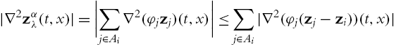
because {φj}![]() is a partition of unity. Now we find (since all norms on polynomials are equivalent, #Aj⩽c
is a partition of unity. Now we find (since all norms on polynomials are equivalent, #Aj⩽c![]() and Lemma 6.1.8) that
and Lemma 6.1.8) that
|∇2zαλ(t,x)|⩽c∑j∈Ai‖zi−zj‖L∞(Qi)r2i⩽cλ.

Concerning the time derivative for (t,x)∈Qi![]() since zi
since zi![]() is constant in time we find that
is constant in time we find that
|∂tzαλ(t,x)|=|∂t∑j∈Ai(φjzj)(t,x)|⩽∑j∈Ai|∂t(φj)(zj−zi)(t,x)|⩽∑j∈Ai‖zi−zj‖L∞(Qi)αr2i⩽cλα.

The zero order term is estimated by Poincaré's inequality; first in time and then in space
r−20‖zαλ‖L∞(14I0;L∞(14B0))⩽cα‖∂tzαλ‖L∞(14Q0)+cr−20‖zαλ‖L1(14I0;L∞(14B0))⩽cλ+c‖∇2zαλ‖L∞(14Q0)+cr−20‖zαλ‖L1(14Q0).

This implies, by the norm equivalence of polynomials, Jensen's inequality, Lemma 6.1.9 and (6.1.13),
r−10‖∇zαλ‖L∞(14Q0)+r−20‖zαλ‖L∞(14Q0)⩽cλ+r−20‖z‖Lσ(13Q0)⩽cλ.
□
The next lemma will control the time error we get when we apply the truncation as a test function.
Lemma 6.1.11

Proof
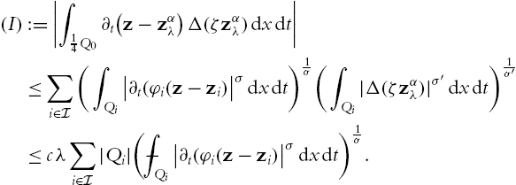
We use Hölder's inequality and Lemma 6.1.10 to derive
(I):=|∫14Q0∂t(z−zαλ)Δ(ζzαλ)dxdt|⩽∑i∈I(∫Qi|∂t(φi(z−zi)|σdxdt)1σ(∫Qi|Δ(ζzαλ)|σ′dxdt)1σ′⩽cλ∑i∈I|Qi|(⨍Qi|∂t(φi(z−zi)|σdxdt)1σ.
Combining this with (6.1.17), (6.1.9) and (6.1.10) yields
(I)⩽cλ∑i∈I|Qi|(α−1(⨍Qj|∇2z|σdxdt)1σ+(⨍Qj|∂tz|σdxdt)1α)⩽cα−1λ2∑i∈I|Qi|⩽cα−1λ2|Oαλ|,

using the local finiteness of the {Qi}![]() in the final step. □
in the final step. □
Theorem 6.1.24
Let 1<p<∞![]() with p,p′>σ
with p,p′>σ![]() . Let wm
. Let wm![]() and Hm
and Hm![]() satisfy ∂tΔwm=−divdivHm
satisfy ∂tΔwm=−divdivHm![]() in the sense of distributions D′(12Q0)
in the sense of distributions D′(12Q0)![]() , see (6.1.5). Further assume that wm
, see (6.1.5). Further assume that wm![]() is a weak null sequence in Lp(12I0;W2,p(12B0))
is a weak null sequence in Lp(12I0;W2,p(12B0))![]() and a strong null sequence in Lσ(12Q0)
and a strong null sequence in Lσ(12Q0)![]() . Further, assume that Hm=H1m+H2m
. Further, assume that Hm=H1m+H2m![]() such that H1m
such that H1m![]() is a weak null sequence in Lp′(Q0)
is a weak null sequence in Lp′(Q0)![]() and H2m
and H2m![]() converges strongly to zero in Lσ(Q0)
converges strongly to zero in Lσ(Q0)![]() . Define zm:=ΔΔ−212B0Δwm
. Define zm:=ΔΔ−212B0Δwm![]() pointwise in time on 12I0
pointwise in time on 12I0![]() . Then there is a double sequence (λm,k)⊂R+
. Then there is a double sequence (λm,k)⊂R+![]() and k0∈N
and k0∈N![]() such that
such that
(a) 22k⩽λm,k⩽22k+1![]()
such that the double sequence zm,k:=zαm,kλm,k![]() with αm,k:=λ2−pm,k
with αm,k:=λ2−pm,k![]() satisfies the following properties for all k⩾k0
satisfies the following properties for all k⩾k0![]()
(b) {zm,k≠z}⊂Om,k:=Oαm,kλm,k![]() ,
,
(c) ‖∇2zm,k‖L∞(14Q0)⩽cλm,k![]() ,
,
(d) zm,k→0![]() and ∇zm,k→0
and ∇zm,k→0![]() in L∞(14Q0)
in L∞(14Q0)![]() for m→∞
for m→∞![]() and k fixed,
and k fixed,
(e) ∇2zm,k⇀⁎0![]() in L∞(14Q0)
in L∞(14Q0)![]() for m→∞
for m→∞![]() and k fixed,
and k fixed,
(f) We have for all ζ∈C∞0(14Q0)![]()
|∫(∂t(zm−zm,k))⋅Δ(ζzm,k)dxdt|⩽cλpm,k|Om,k|,

(g) limsupm→∞λpm,k|Om,k|⩽c2−ksupm(‖∇2zm‖p+c‖H1m‖1p−1p′)![]() .
.
Proof
Let us assume that λm,k![]() satisfies (a). We will choose the precise values of λm,k
satisfies (a). We will choose the precise values of λm,k![]() later. Due to Lemma 6.1.3 we have zm⇀0
later. Due to Lemma 6.1.3 we have zm⇀0![]() in Lp(14I0;W2,p(14B0))
in Lp(14I0;W2,p(14B0))![]() ; this is due to the fact that the operator w↦ΔΔ−212B0Δw=z
; this is due to the fact that the operator w↦ΔΔ−212B0Δw=z![]() is linear and continuous in Lp(14I0;W2,p(14B0))
is linear and continuous in Lp(14I0;W2,p(14B0))![]() . Then the properties (b) and (c) follow from Lemma 6.1.10. Moreover, Corollary 6.1.1 ensures that the strong convergence in Lσ(12Q0)
. Then the properties (b) and (c) follow from Lemma 6.1.10. Moreover, Corollary 6.1.1 ensures that the strong convergence in Lσ(12Q0)![]() transfers from wm
transfers from wm![]() to zm
to zm![]() . By Lemma 6.1.9 we get the same for zm,k
. By Lemma 6.1.9 we get the same for zm,k![]() and that the sequence ∇2zm,k
and that the sequence ∇2zm,k![]() is, for fixed k and s, bounded in Ls(14Q0)
is, for fixed k and s, bounded in Ls(14Q0)![]() . The combination of these convergence properties implies (by interpolation) (d). Moreover, the boundedness of ∇2zm,k
. The combination of these convergence properties implies (by interpolation) (d). Moreover, the boundedness of ∇2zm,k![]() in Ls(14Q0)
in Ls(14Q0)![]() implies the weak convergence of a subsequence. Since (d) ensures that the limit is zero, we get, by the usual arguments, weak convergence of the whole sequence. This proves (e). Moreover, (f) follows by Lemma 6.1.11 and the choice of αm,k
implies the weak convergence of a subsequence. Since (d) ensures that the limit is zero, we get, by the usual arguments, weak convergence of the whole sequence. This proves (e). Moreover, (f) follows by Lemma 6.1.11 and the choice of αm,k![]() .
.
It remains to choose 22k⩽λm,k⩽22k+1![]() such that (g) holds. We use the decomposition
such that (g) holds. We use the decomposition
∂tzm=ΔΔ−212B0divdivHm=ΔΔ−212B0divdivH1m+ΔΔ−212B0divdivH2m=:h1m+h2m.

We decompose
Om,k={Mαm,kσ(χ13Q0|∇2zm,k|)>λm,k}∪{αm,kMαm,kσ(χ13Q0|∂tzm|)>λm,k}⊂{Mαm,kσ(χ13Q0|∇2zm,k|)>λm,k}∪{αm,kMαm,kσ(χ13Q0|h1m|)>12λm,k}∪{αm,kMαm,kσ(χ13Q0|h2m|)>12λm,k}=:I∪II∪III.

Define
gm:=2Mαm,kσ(χ13Q0|∇2zm|)+(2Mαm,kσ(χ13Q0|h1m|))1p−1.
Then by the boundedness of Mσ![]() on Lp
on Lp![]() and Lp′
and Lp′![]() (using p,p′>σ
(using p,p′>σ![]() ), as well as Corollary 6.1.3, we have
), as well as Corollary 6.1.3, we have
‖gm‖p⩽‖2Mαm,kσ(χ13Q0|∇2zm|)‖p+‖(2Mαm,kσ(χ13Q0|h1m|))1p−1‖p=‖2Mαm,kσ(χ13Q0|∇2zm|)‖p+‖2Mαm,kσ(χ13Q0|h1m|)‖1p−1p′⩽c‖∇2zm‖Lp(13Q0)+c‖h1m‖1p−1Lp′(12Q0)⩽c‖∇2zm‖Lp(13Q0)+c‖H1m‖1p−1Lp′(12Q0).

Let K:=supm(‖∇2zm‖p+c‖h1m‖1p−1p′)![]() . In particular, ‖gm‖p⩽K
. In particular, ‖gm‖p⩽K![]() uniformly in k. Note that
uniformly in k. Note that
I∪II={Mαm,kσ(χ13Q0|∇2zm,k|)>λm,k}∪{(Mαm,kσ(χ13Q0|h1m|))1p−1>λm,k}⊂{2Mαm,kσ(χ13Q0|∇2zm,k|)+(2Mαm,kσ(χ13Q0|h1m|))1p−1>λm,k}={gm>λm,k}.

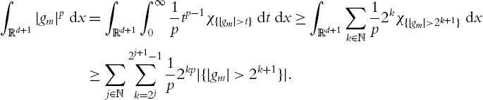
We estimate
∫Rd+1|gm|pdx=∫Rd+1∫∞01ptp−1χ{|gm|>t}dtdx⩾∫Rd+1∑k∈N1p2kχ{|gm|>2k+1}dx⩾∑j∈N2j+1−1∑k=2j1p2kp|{|gm|>2k+1}|.
For fixed m,j![]() the sum over k involves 2j
the sum over k involves 2j![]() summands and not all of them can be large. Consequently there exists λm,k∈{22k+1,…,22k+1}
summands and not all of them can be large. Consequently there exists λm,k∈{22k+1,…,22k+1}![]() , such that
, such that
λpm,k|{|gm|>λm,k}|⩽c2−kKp
uniformly in m and k, and hence
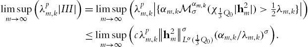
λpm,k|I∪II|⩽λpm,k|{gm>λm,k}|⩽c2−kKp.
On the other hand, from the weak-Lσ![]() estimate for Mαm,kσ
estimate for Mαm,kσ![]() we see that
we see that
limsupm→∞(λpm,k|III|)=limsupm→∞(λpm,k|{αm,kMαm,kσ(χ13Q0|h2m|)>12λm,k}|)⩽limsupm→∞(cλpm,k‖h2m‖σLσ(13Q0)(αm,k/λm,k)σ).
Since 22k+1⩽λm,k⩽22k+1![]() , αm,k=λ2−pm,k
, αm,k=λ2−pm,k![]() and h2m→0
and h2m→0![]() in Lσ(12Q0)
in Lσ(12Q0)![]() (which is a consequence of H2m→0
(which is a consequence of H2m→0![]() in Lσ(12Q0)
in Lσ(12Q0)![]() and Corollary 6.1.3), it follows that
and Corollary 6.1.3), it follows that
limsupm→∞(λpm,k|III|)=0.
Theorem 6.1.25
Let 1<p<∞![]() with p,p′>σ
with p,p′>σ![]() . Let um
. Let um![]() and Gm
and Gm![]() satisfy ∂tum=−divGm
satisfy ∂tum=−divGm![]() in the sense of distributions D′div(Q0)
in the sense of distributions D′div(Q0)![]() . Assume that um
. Assume that um![]() is a weak null sequence in Lp(I0;W1,p(B0))
is a weak null sequence in Lp(I0;W1,p(B0))![]() and a strong null sequence in Lσ(Q0)
and a strong null sequence in Lσ(Q0)![]() and bounded in L∞(I0,T;Lσ(B0))
and bounded in L∞(I0,T;Lσ(B0))![]() . Further assume that Gm=G1m+G2m
. Further assume that Gm=G1m+G2m![]() such that G1m
such that G1m![]() is a weak null sequence in Lp′(Q0)
is a weak null sequence in Lp′(Q0)![]() and G2m
and G2m![]() converges strongly to zero in Lσ(Q0)
converges strongly to zero in Lσ(Q0)![]() . Then there is a double sequence (λm,k)⊂R+
. Then there is a double sequence (λm,k)⊂R+![]() and k0∈N
and k0∈N![]() with
with
(a) 22k⩽λm,k⩽22k+1![]()
such that the double sequences um,k:=uαm,kλm,k∈L1(Q0)![]() , αm,k:=λ2−pm,k
, αm,k:=λ2−pm,k![]() and Om,k:=Oαm,kλm,k
and Om,k:=Oαm,kλm,k![]() (defined in Theorem 6.1.24) satisfy the following properties for all k⩾k0
(defined in Theorem 6.1.24) satisfy the following properties for all k⩾k0![]() .
.
(b) um,k∈Ls(14I0;W1,s0,div(16B0))![]() for all s<∞
for all s<∞![]() and supp(um,k)⊂16Q0
and supp(um,k)⊂16Q0![]() .
.
(c) um,k=um![]() a.e. on 18Q0∖Om,k
a.e. on 18Q0∖Om,k![]() .
.
(d) ‖∇um,k‖L∞(14Q0)⩽cλm,k![]() .
.
(e) um,k→0![]() in L∞(14Q0)
in L∞(14Q0)![]() for m→∞
for m→∞![]() and k fixed.
and k fixed.
(f) ∇um,k⇀⁎0![]() in L∞(14Q0)
in L∞(14Q0)![]() for m→∞
for m→∞![]() and k fixed.
and k fixed.
(g) limsupm→∞λpm,k|Om,k|⩽c2−k.![]()
(h) limsupm→∞|∫Gm:∇um,kdxdt|⩽cλpm,k|Om,k|![]() .
.
Proof
We define, pointwise in time on I0![]() ,
,
˜um:=γum−BogB0∖12B0(∇γ⋅um),wm:=curl−1˜um,zm:=ΔΔ−212Q0Δwm,

where γ∈C∞0(Q0)![]() with χ12Q0⩽γ⩽χQ0
with χ12Q0⩽γ⩽χQ0![]() . Then we apply Theorem 6.1.24 to the sequence zm
. Then we apply Theorem 6.1.24 to the sequence zm![]() . Finally, let
. Finally, let
um,k:=curl(ζzm,k)+curl(ζ(wm−zm)),
where ζ∈C∞0(16Q0)![]() with χ18Q0⩽ζ⩽χ16Q0
with χ18Q0⩽ζ⩽χ16Q0![]() . This means on 18Q0
. This means on 18Q0![]() we have
we have
um,k=um+curl(zm,k−zm).
Note that curl(wm−zm)![]() is harmonic (in space) on 12Q0
is harmonic (in space) on 12Q0![]() and bounded in time, due to the assumption that um
and bounded in time, due to the assumption that um![]() is bounded uniformly in L∞(I0;Lσ(B0))
is bounded uniformly in L∞(I0;Lσ(B0))![]() , which transfers to wm
, which transfers to wm![]() and zm
and zm![]() by Lemma 6.1.1 and 6.1.4. This allows us to estimate the higher order spaces derivatives on 14Q0
by Lemma 6.1.1 and 6.1.4. This allows us to estimate the higher order spaces derivatives on 14Q0![]() by lower order ones on 12Q0
by lower order ones on 12Q0![]() . This, (6.1.19) and Theorem 6.1.24 immediately imply all the claimed properties except (h).
. This, (6.1.19) and Theorem 6.1.24 immediately imply all the claimed properties except (h).
The claim of (g) follows exactly as (g) of Theorem 6.1.24.
Let us prove (h). It follows by simple density arguments that um,k![]() is an admissible test function for the equation ∂tum=−divGm
is an admissible test function for the equation ∂tum=−divGm![]() . We thus obtain
. We thus obtain
∫Gm:∇um,kdxdt=∫∂tum⋅um,kdxdt=∫(∂tcurlwm)⋅curl(ζzm,k)dxdt+∫(∂tcurlwm)⋅curl(ζ(wm−zm))dxdt=−∫(∂tzm)⋅Δ(ζzm,k)dxdt−∫(∂tzm)⋅Δ(ζ(wm−zm))dxdt=:T1+T2.

Here we took into account curlcurlwm=−Δwm![]() (due to divwm=0
(due to divwm=0![]() ) and Δwm=Δzm
) and Δwm=Δzm![]() . By assumption Gm
. By assumption Gm![]() is bounded in Lσ(Q0)
is bounded in Lσ(Q0)![]() . Using regularity properties of harmonic functions (for wm−zm
. Using regularity properties of harmonic functions (for wm−zm![]() ) as well as Lemma 6.1.3 and Lemma 6.1.1 we gain (after choosing a subsequence)
) as well as Lemma 6.1.3 and Lemma 6.1.1 we gain (after choosing a subsequence)
(⨍Q0|Δ(ζ(wm−zm))|σ′dxdt)1σ′⩽cr−20(⨍14Q0|wm−zm|3σ3+σdxdt)3+σ3σ⩽cr−20(⨍12Q0|wm|3σ3+σdxdt)3+σ3σ⩽cr−30(⨍Q0|˜um|σdxdt)1σ⟶0asm→∞.

Since, additionally, ∂tzm![]() is uniformly bounded in Lσ(12Q0)
is uniformly bounded in Lσ(12Q0)![]() by Lemma 6.1.3, we have T2→0
by Lemma 6.1.3, we have T2→0![]() as m→∞
as m→∞![]() . Furthermore, there holds
. Furthermore, there holds
T1=∫(∂t(zm−zm,k))⋅Δ(ζzm,k)dxdt+∫(∂tzm,k)⋅Δ(ζzm,k)dxdt=:T1,1+T1,2,

where the first term can be bounded using Theorem 6.1.24 (f). So it remains to show that
T1,2:=∫(∂tzm,k)⋅Δ(ζzm,k)dxdt⟶0asm→∞.

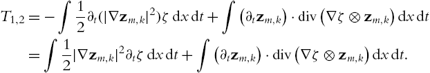
We have
T1,2=−∫12∂t(|∇zm,k|2)ζdxdt+∫(∂tzm,k)⋅div(∇ζ⊗zm,k)dxdt=∫12|∇zm,k|2∂tζdxdt+∫(∂tzm,k)⋅div(∇ζ⊗zm,k)dxdt.
The first term is estimated by Theorem 6.1.24(d). For the second we use Lemma 6.1.9 and Lemma 6.1.3 (s=σ![]() ) to find
) to find
∫|∂tzm,k||div(∇ζ⊗zm,k)|dxdt⩽c(∫13Q0|Gm|σ+|∇2zm|σdxdt)1σ(∫13Q0|∇zm,k|σ′+|zm,k|σ′dxdt)1σ′.

Now because Gm![]() and ∇2zm
and ∇2zm![]() are uniformly bounded in Lσ(12Q0)
are uniformly bounded in Lσ(12Q0)![]() we find by Theorem 6.1.24 (d), that
we find by Theorem 6.1.24 (d), that
limm→∞T1,2=0,
which proves the claim of (h). □
The following corollary is useful in the application of the solenoidal Lipschitz truncation.
Corollary 6.1.4
Let all assumptions of Theorem 6.1.25 be satisfied with ζ∈C∞0(16Q0)![]() with χ18Q0⩽ζ⩽χ16Q0
with χ18Q0⩽ζ⩽χ16Q0![]() as in the proof of Theorem 6.1.25. If additionally um
as in the proof of Theorem 6.1.25. If additionally um![]() is uniformly bounded in L∞(I0,Lσ(B0))
is uniformly bounded in L∞(I0,Lσ(B0))![]() , then for every K∈Lp′(16Q0)
, then for every K∈Lp′(16Q0)![]()
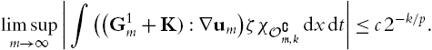
limsupm→∞|∫((G1m+K):∇um)ζχO∁m,kdxdt|⩽c2−k/p.
Proof
It follows from (f), (g) and (h) of Theorem 6.1.25 that
limsupm→∞|∫(Gm+K):∇um,kdxdt|⩽cλpm,k|Om,k|⩽c2−k.

Recall that um,k=curl(ζzm,k)+curl(ζ(wm−zm))![]() . So, by Theorem 6.1.24, we have zm,k,∇zm,k→0
. So, by Theorem 6.1.24, we have zm,k,∇zm,k→0![]() in L∞(14Q0)
in L∞(14Q0)![]() as m→∞
as m→∞![]() with k fixed. Since um
with k fixed. Since um![]() is a strong null sequence in Lσ(Q0)
is a strong null sequence in Lσ(Q0)![]() and is bounded in L∞(I0,Lσ(B0))
and is bounded in L∞(I0,Lσ(B0))![]() we see that um→0
we see that um→0![]() strongly in Ls(I0,Lσ(B0))
strongly in Ls(I0,Lσ(B0))![]() for any s∈(1,∞)
for any s∈(1,∞)![]() . By continuity of the Bogovskiĭ operator (see Theorem 2.1.6 with A(t)=B(t)=tσ
. By continuity of the Bogovskiĭ operator (see Theorem 2.1.6 with A(t)=B(t)=tσ![]() ) we have the same convergence for ˜um
) we have the same convergence for ˜um![]() . Now, Lemma 6.1.1 implies wm=curl−1˜um→0
. Now, Lemma 6.1.1 implies wm=curl−1˜um→0![]() in Ls(I0,W1,σ(R3))
in Ls(I0,W1,σ(R3))![]() . Using zm:=ΔΔ−212Q0Δwm
. Using zm:=ΔΔ−212Q0Δwm![]() and Corollary 6.1.1 we also have zm→0
and Corollary 6.1.1 we also have zm→0![]() in Ls(I0,W1,σ(R3))
in Ls(I0,W1,σ(R3))![]() . Since zm−wm
. Since zm−wm![]() is harmonic on 14Q0
is harmonic on 14Q0![]() , we have zm−wm→0
, we have zm−wm→0![]() in Ls(I0,W2,s(16B0))
in Ls(I0,W2,s(16B0))![]() . These convergences imply that
. These convergences imply that
∇um,k=ζ∇curlzm,k+am,k,
with am,k→0![]() in Ls(16Q0)
in Ls(16Q0)![]() as m→∞
as m→∞![]() with k fixed. This, the boundedness of Gm
with k fixed. This, the boundedness of Gm![]() in Lσ(16Q0)
in Lσ(16Q0)![]() , K∈Lp′(16Q0)
, K∈Lp′(16Q0)![]() and (6.1.20) imply (using s>σ′
and (6.1.20) imply (using s>σ′![]() )
)
limsupm→∞|∫((Gm+K):∇curlzm,k)ζdxdt|⩽c2−k.

Since Gm=G1m+G2m![]() , G2m→0
, G2m→0![]() in Lσ(16Q0)
in Lσ(16Q0)![]() and zm,k⇀0
and zm,k⇀0![]() in Lσ′(16Qz)
in Lσ′(16Qz)![]() for m→∞
for m→∞![]() and k fixed, we have
and k fixed, we have
limsupm→∞|∫((G1m+K):∇curlzm,k)ζdxdt|⩽c2−k.

The boundedness of G1m![]() and K in Lp′(16Q0)
and K in Lp′(16Q0)![]() and Theorem 6.1.24 and (g) prove
and Theorem 6.1.24 and (g) prove
limsupm→∞|∫((G1m+K):∇curlzm,k)ζχOm,kdxdt|⩽c2−k/p.

This, together with (6.1.21) and zm,k=zm![]() in O∁m,k
in O∁m,k![]() yield
yield
limsupm→∞|∫((G1m+K):∇curlzm)ζχO∁m,kdxdt|⩽c2−k/p.

Recall that zm−wm→0![]() in Ls(I0,W2,s(16B0))
in Ls(I0,W2,s(16B0))![]() for any s∈(1,∞)
for any s∈(1,∞)![]() . This and the boundedness of G1m
. This and the boundedness of G1m![]() in Lp′(Q0)
in Lp′(Q0)![]() allows us to replace zm
allows us to replace zm![]() in the previous integral by wm
in the previous integral by wm![]() . Now curlwm=um
. Now curlwm=um![]() proves the claim. □
proves the claim. □
The next corollary follows by combining Lemma 6.1.9, Lemma 6.1.10, Theorem 6.1.24 (g) (with α=1![]() ) and the continuity of curl−1
) and the continuity of curl−1![]() with a scaling procedure.
with a scaling procedure.
Corollary 6.1.5
For some σ>0![]() let u∈Lσ(I0;W1,σdiv(B0))∩L∞(I;Lσ(B0))
let u∈Lσ(I0;W1,σdiv(B0))∩L∞(I;Lσ(B0))![]() with ∂tu=divH
with ∂tu=divH![]() in D′div(Q0)
in D′div(Q0)![]() for some H∈Lσ(Q0)
for some H∈Lσ(Q0)![]() . Then for every m0≫1
. Then for every m0≫1![]() and γ>0
and γ>0![]() there exist λ∈[2m0γ,22m0γ]
there exist λ∈[2m0γ,22m0γ]![]() and a function uλ
and a function uλ![]() with the following properties.
with the following properties.
(a) It holds uλ∈L∞(I0,W1,∞0,div(B0))![]() with ‖∇uλ‖∞⩽cλ
with ‖∇uλ‖∞⩽cλ![]() .
.
(b) We have
λσLd+1(12Q0∩{uλ≠u})|Q0|⩽cm0(⨍Q0r−σ0|u|σ+|∇u|σdxdt+⨍Q0|H|σdxdt).

(c) It holds
⨍Q0|uλ|σdxdt⩽c(⨍Q0|u|σ+⨍Q0rσ0|H|σdxdt),⨍Q0|∇uλ|σdxdt⩽c(⨍Q0r−σ0|u|σ+|∇u|σdxdt+⨍Q0|H|σdxdt).

(d) We have ∂t(u−uλ)∈Lσ′(12I0,W−1,σ′(12B0))![]() and
and
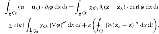
−⨍12Q0(u−uλ)⋅∂tφdxdt⩽c(κ)∫12Q0χ{uλ≠u}|∇φ|σ′dxdt+κ(⨍Q0r−σ0|u|σ+|∇u|σ+|H|σdxdt)

for all φ∈C∞0(12Q0)![]() and all κ>0
and all κ>0![]() .
.
Proof
We apply the arguments used in the proof of Theorem 6.1.25 to the constant sequence u with the choice α=1![]() . So we set
. So we set
uλ:=curl(ζzλ)+curl(ζ(w−z)),
where ζ∈C∞0(16Q0)![]() with χ18Q0⩽ζ⩽χ16Q0
with χ18Q0⩽ζ⩽χ16Q0![]() . Hence, in 18Q0
. Hence, in 18Q0![]() we have
we have
uλ=u+curl(zλ−z).
We immediately obtain the claim of (a). As a consequence of the Lemmas 6.1.1, 6.1.4 and 6.1.9 we obtain the inequalities
⨍Q|uλ|σdxdt⩽c(⨍Q0|u|σ+⨍Qrσ0|∂tz|σdxdt),⨍Q0|∇uλ|σdxdt⩽c(⨍Q0r−σ0|u|σ+|∇u|σdxdt+⨍Q|∂tz|σdxdt),

claimed in c). Finally we can replace ∂tz![]() by H on account of Lemma 6.1.3.
by H on account of Lemma 6.1.3.
It remains to find good levels. We define for some s∈(1,max{σ,σ′})![]()
Oλ:={Ms(χ13Q0|∇2z|)>λ}∪{Ms(χ13Q0|H|)>λ},g:=Ms(χ13Q0|∇2z|)+Ms(χ13Q0|H|).

It now follows from the continuity of Ms![]() in (5.2.4), together with Lemmas 6.1.1 and 6.1.4
in (5.2.4), together with Lemmas 6.1.1 and 6.1.4
∫Rd+1|g|σdx⩽c(∫Q0r−σ0|u|σ+|∇u|σdxdt+∫Q0|H|σdxdt).

Furthermore, the following holds for every m0∈N![]() and every γ>0
and every γ>0![]()
∫Rd+1|g|σdx=∫Rd+1∫∞01σtσ−1χ{|g|>t}dtdx⩾∫Rd+12m0−1∑m=m01σ(2mγ)σχ{|g|>γ2m+1}dx.

So, there is m1∈{m0,...,2m0−1}![]() such that
such that
∫Rd+1(2m1γ)σχ{|g|>γ2m1+1}dx⩽cm0∫Rd+1|g|σdx.

Setting λ=γ2m1+1![]() yields
yields
λσ|13Q0∩{|g|>λ}|⩽cm0∫Rd+1|g|σdx.

Combining this with (6.1.23) gives the estimate in b) due to the definition of Oλ![]() .
.
Finally, we prove d). We have uλ−u=curl(zλ−z)![]() in 18Q0
in 18Q0![]() such that Lemma 6.1.3 and 6.1.9 imply ∂t(uλ−u)∈Lσ′(18I0,W−1,σ′(18B0))
such that Lemma 6.1.3 and 6.1.9 imply ∂t(uλ−u)∈Lσ′(18I0,W−1,σ′(18B0))![]() . Moreover, we have for φ∈C∞0(18Q0)
. Moreover, we have for φ∈C∞0(18Q0)![]()
−∫18Q0(u−uλ)⋅∂tφdxdt=∫18Q0χOλ∂t(z−zλ)⋅curlφdxdt⩽c(κ)∫12Q0χOλ|∇φ|σ′dxdt+κ(⨍Q0|∂t(zλ−z)|σdxdt),
as a consequence of Young's inequality. Applying Lemmas 6.1.3, 6.1.4 and 6.1.9 yields
⨍Q0|∂t(zλ−z)|σdxdt⩽c(⨍Q0r−σ0|u|σ+|∇u|σdxdt+⨍Q0|H|σdxdt).

So we have shown the estimate claimed in (d) on 18Q0![]() .
.
A simple scaling argument allows us the obtain all the estimates on 12Q0![]() . □
. □
Remark 6.1.10
The higher dimensional case
For general dimensions, the solenoidal Lipschitz truncation is best understood in terms of differential forms. We start with ˜u![]() as given in (6.1.3). Now, we have to find w such that curlw=˜u
as given in (6.1.3). Now, we have to find w such that curlw=˜u![]() and divw=0
and divw=0![]() . Let us define the 1-form α in Rd
. Let us define the 1-form α in Rd![]() associated to the vector field ˜u
associated to the vector field ˜u![]() by α:=∑i˜uidxi
by α:=∑i˜uidxi![]() . Then we need to find a 2-form G such that d⁎G=α
. Then we need to find a 2-form G such that d⁎G=α![]() and dG=0
and dG=0![]() , where d is the outer derivative and d⁎
, where d is the outer derivative and d⁎![]() its adjoint by the scalar product for k-forms. Similar to w=curl−1˜u=curlΔ−1˜u
its adjoint by the scalar product for k-forms. Similar to w=curl−1˜u=curlΔ−1˜u![]() we get G by G:=dΔ−1α
we get G by G:=dΔ−1α![]() . Since we are on the whole space, Δ−1
. Since we are on the whole space, Δ−1![]() can be constructed by mollification with c|x|2−d
can be constructed by mollification with c|x|2−d![]() . Thus, we have
. Thus, we have
G(x)=(dΔ−1α)(x)=d∑i(∫Rdui(y)|x−y|d−2dy)dxi.

Let us explain how to substitute the equation ∂tΔw=−curldivG![]() , see (6.1.4). Instead of test functions ψ with divψ=0
, see (6.1.4). Instead of test functions ψ with divψ=0![]() we use the associated 1-forms β=∑iψidxi
we use the associated 1-forms β=∑iψidxi![]() with d⁎β=0
with d⁎β=0![]() . Thus there exists a 2-form γ with d⁎γ=0
. Thus there exists a 2-form γ with d⁎γ=0![]() . Then
. Then
〈∂t˜u,ψ〉=〈∂tα,β〉=〈∂td⁎G,d⁎γ〉=〈∂tdd⁎G,γ〉=〈−∂tΔG,γ〉,
where we used −Δ=dd⁎+d⁎d![]() and dα=0
and dα=0![]() in the last step. Note that −Δ applied to the form G is the same as −Δ applied to the vector field of all components of G. Now we define w as the associated vector field (with (d2)
in the last step. Note that −Δ applied to the form G is the same as −Δ applied to the vector field of all components of G. Now we define w as the associated vector field (with (d2)![]() components) of G and we arrive again at an equation for ∂tΔw
components) of G and we arrive again at an equation for ∂tΔw![]() . This concludes the construction; the rest can be done exactly as for dimension three. The restriction p>65
. This concludes the construction; the rest can be done exactly as for dimension three. The restriction p>65![]() used in this section will change to 2dd+2
used in this section will change to 2dd+2![]() .
.
6.2 A -Stokes approximation – evolutionary case
By A![]() we denote a symmetric, elliptic tensor, i.e.
we denote a symmetric, elliptic tensor, i.e.
c0|τ|2⩽A(τ,τ)⩽c1|τ|2for allτ∈Rd×d.
We set |A|:=c1/c0![]() . Let B⊂Rd
. Let B⊂Rd![]() be a ball and J=(t0,t1)
be a ball and J=(t0,t1)![]() a bounded interval. We set Q=J×B
a bounded interval. We set Q=J×B![]() . For a function w∈L1(Q)
. For a function w∈L1(Q)![]() with ∂tw∈Lq′(J;W−1,q′(B))
with ∂tw∈Lq′(J;W−1,q′(B))![]() we introduce the unique function Hw∈Lq′0(Q)
we introduce the unique function Hw∈Lq′0(Q)![]() with
with
∫Qw⋅∂tφdxdt=∫QHw:∇φdxdt

for all φ∈C∞0,div(Q)![]() . We begin with a variational inequality for the non-stationary A
. We begin with a variational inequality for the non-stationary A![]() -Stokes system.
-Stokes system.
Lemma 6.2.1
Suppose that (6.2.24) holds and that q>1![]() . There holds for every u∈Cw([t0,t1];L1(B))∩Lq(J;W1,q(B))
. There holds for every u∈Cw([t0,t1];L1(B))∩Lq(J;W1,q(B))![]() with u(t0,⋅)=0
with u(t0,⋅)=0![]() a.e.
a.e.
⨍Q|∇u|qdxdt⩽csupξ∈C∞0,div(Q)[⨍Q(A(ε(u),ε(ξ))−u⋅∂tξ)dxdt−⨍Q(|∇ξ|q′+|Hξ|q′)dxdt],

where c only depends on A![]() , q and d.
, q and d.
Proof
Duality arguments show that
1q⨍Q|∇u|qdxdt=supG∈Lq′(Q)[⨍Q∇u:Gdxdt−1q′⨍Q|G|q′dxdt].

For a given G∈Lq′(Q)![]() let zG
let zG![]() be the unique Lq′(J;W1,q′0,div(B))
be the unique Lq′(J;W1,q′0,div(B))![]() -solution to
-solution to
⨍Qz⋅∂tξdxdt+∫QA(ε(z),ε(ξ))dxdt=∫QG:∇ξdxdt

for all ξ∈C∞0,div((t0,t1]×B)![]() . This is a backward parabolic equation with end datum zero. We have that ∂tzG∈Lq′(J;W−1,q′div(B))
. This is a backward parabolic equation with end datum zero. We have that ∂tzG∈Lq′(J;W−1,q′div(B))![]() , so test-functions can be chosen from the space Lq(J;W1,q0,div(B))
, so test-functions can be chosen from the space Lq(J;W1,q0,div(B))![]() . Due to Theorem B.3.50 (which can be applied to ˜z˜G(t,⋅)=zG(t1−t,⋅)
. Due to Theorem B.3.50 (which can be applied to ˜z˜G(t,⋅)=zG(t1−t,⋅)![]() , where ˜G(t,⋅)=G(t1−t,⋅)
, where ˜G(t,⋅)=G(t1−t,⋅)![]() ) this solution satisfies
) this solution satisfies
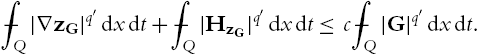
⨍Q|∇zG|q′dxdt+⨍Q|HzG|q′dxdt⩽c⨍Q|G|q′dxdt.
In other words, the mapping Lq′(B)∋G↦zG∈Lq′(J;W1,q′0,div(B))![]() is continuous. This and u(t0,⋅)=0
is continuous. This and u(t0,⋅)=0![]() yield (using u as a test-function in (6.2.25))
yield (using u as a test-function in (6.2.25))
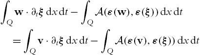
⨍Q|∇u|qdxdt⩽csupG∈Lq′(Q)[⨍QA(ε(u),ε(zG))dxdt−⨍Q∂tzG⋅udxdt−⨍Q(|∇zH|q′+|HzG|q′)dxdt]⩽csupξ∈C∞0,div(Q)[⨍QA(ε(u),ε(ξ))dxdt−⨍Qu⋅∂tξdxdt−⨍Q(|∇ξ|q′+|Hξ|q′)dxdt],

which yields the claim. □
Let us now state the A![]() -Stokes approximation. In the following let B
-Stokes approximation. In the following let B![]() be a ball with radius r and J an interval with length 2r2
be a ball with radius r and J an interval with length 2r2![]() . Let ˜Q
. Let ˜Q![]() denote either Q=J×B
denote either Q=J×B![]() or 2Q. We use similar notations for ˜J
or 2Q. We use similar notations for ˜J![]() and ˜B
and ˜B![]() .
.
Theorem 6.2.26
Suppose that (6.2.24) holds. Let v∈Lqs(2˜J;W1,qsdiv(2˜B))![]() , q,s>1
, q,s>1![]() , be an almost A
, be an almost A![]() -Stokes solution in the sense that
-Stokes solution in the sense that
|⨍2Qv⋅∂tξdxdt−⨍2QA(ε(v),ε(ξ))dxdt|⩽δ⨍2˜Q|ε(v)|dxdt‖∇ξ‖∞

for all ξ∈C∞0,div(2Q)![]() and some small δ>0
and some small δ>0![]() . Then the unique solution w∈Lq(J;W1,q0,div(B))
. Then the unique solution w∈Lq(J;W1,q0,div(B))![]() to
to
∫Qw⋅∂tξdxdt−∫QA(ε(w),ε(ξ))dxdt=∫Qv⋅∂tξdxdt−∫QA(ε(v),ε(ξ))dxdt
for all ξ∈C∞0,div([t0,t1)×B)![]() satisfies
satisfies
⨍Q|wr|qdxdt+⨍Q|∇w|qdxdt⩽κ(⨍2˜Q|∇v|qsdxdt)1s.

It holds κ=κ(q,s,δ)![]() and limδ→0κ(q,s,δ)=0
and limδ→0κ(q,s,δ)=0![]() . The function h:=v−w
. The function h:=v−w![]() is called the A
is called the A![]() -Stokes approximation of v.
-Stokes approximation of v.
Remark 6.2.11
From the proof of Theorem 6.2.26 we have the following stability result, choosing p=qs=q![]() .
.
⨍Q|wr|pdxdt+⨍Q|∇w|pdxdt⩽c⨍2˜Q|∇v|pdxdt.

Indeed κ stays bounded if s→1![]() .
.
Proof
Let w be defined as in (6.2.27). Combining Poincaré's inequality with Lemma 6.2.1 and (6.2.27) shows that
⨍Q|wr|qdxdt+⨍Q|∇w|qdxdt⩽csupξ∈C∞0,div(Q)[⨍QA(ε(v),ε(ξ))dxdt−⨍Qv⋅∂tξdxdt−⨍Q(|∇ξ|q′+|Hξ|q′)dxdt].

In the following let us fix ξ∈C∞0,div(Q)![]() . Let
. Let
γ:=(⨍Q|∇ξ|q′dxdt+⨍Q|Hξ|q′dxdt)1q′,

and m0∈N![]() , m0≫1
, m0≫1![]() . Due to Corollary 6.1.5, applied with σ=q′
. Due to Corollary 6.1.5, applied with σ=q′![]() , we find λ∈[2m0γ,22m0γ]
, we find λ∈[2m0γ,22m0γ]![]() and ξλ∈L∞(4J;W1,∞0,div(4B))
and ξλ∈L∞(4J;W1,∞0,div(4B))![]() such that
such that
‖∇ξλ‖L∞(4Q)⩽cλ,
λq′Ld+1(2Q∩{ξλ≠ξ})|Q|⩽cm0(⨍Q|∇ξ|q′dxdt+⨍Q|Hξ|q′dxdt),

⨍4Q|ξλ|q′dxdt⩽c(⨍Q|ξ|q′dxdt+⨍Qrq′|Hξ|q′dxdt),

⨍4Q|∇ξλ|q′dxdt⩽c(⨍Q|∇ξ|q′dxdt+⨍Q|Hξ|q′dxdt).
Note that ξ can be extended by 0 to 4Q thus the equation
∂tξ=divBogB(∂tξ)=:divHξ
holds on 4Q by the properties of BogB![]() (since Hξ
(since Hξ![]() can be extended as well). For the properties of the Bogovskiĭoperator we refer to Section 2.1, in particular Theorem 2.1.6. Corollary 6.1.5 (d) implies that ∂t(ξ−ξλ)∈Lq′(2J,W−1,q′(2B))
can be extended as well). For the properties of the Bogovskiĭoperator we refer to Section 2.1, in particular Theorem 2.1.6. Corollary 6.1.5 (d) implies that ∂t(ξ−ξλ)∈Lq′(2J,W−1,q′(2B))![]() and
and
∫2J〈∂t(ξ−ξλ),φ〉dt⩽c(κ)∫2Qχ{ξ≠ξλ}|∇φ|qdxdt+κ(∫Q|∇ξ|q′+|Hξ|q′dxdt),

for all φ∈W1,q0(2Q)![]() . For η∈C∞0(2Q)
. For η∈C∞0(2Q)![]() with η≡1
with η≡1![]() on Q, |∇kη|⩽cr−k
on Q, |∇kη|⩽cr−k![]() and |∂t∇k−1η|⩽cr−(k+1)
and |∂t∇k−1η|⩽cr−(k+1)![]() (k=1,2
(k=1,2![]() ) we see that
) we see that
⨍QA(ε(v),ε(ξ))dxdt−⨍Qv⋅∂tξdxdt=2d+2⨍2QA(ε(v),ε(ηξ−Bog2B∖B(∇ηξ)))dxdt−⨍2Qv⋅∂t(ηξ−...)dxdt=2d+2(⨍2QA(ε(v),ε(ηξλ−Bog2B∖B(∇ηξλ)))dxdt+⨍2Q∂tv⋅(ηξλ−...)dxdt)+2d+2⨍2QA(ε(v),ε(η(ξ−ξλ)−Bog2B∖B(∇η(ξ−ξλ))))dxdt+2d+2⨍2Q∂tv⋅(η(ξ−ξλ)−Bog2B∖B(∇η(ξ−ξλ)))dxdt=:2d+2(I+II+III).

Note that the time-derivative of v exists in the W−1,∞div![]() -sense as a consequence of (6.2.26), so all terms are well-defined by the properties of ξλ
-sense as a consequence of (6.2.26), so all terms are well-defined by the properties of ξλ![]() . We have the following inequality on account of the continuity properties of ∇Bog on Lp
. We have the following inequality on account of the continuity properties of ∇Bog on Lp![]() -spaces, (6.2.31), (6.2.32) and Poincaré's inequality (we set ˜ξλ:=ξ−ξλ
-spaces, (6.2.31), (6.2.32) and Poincaré's inequality (we set ˜ξλ:=ξ−ξλ![]() ):
):
⨍2Q|∇Ψλ|q′dxdt:=⨍2Q|∇(η˜ξλ)−∇Bog2B∖B(∇η˜ξλ)|q′dxdt⩽c⨍2Q|∇˜ξλ|q′dxdt+c⨍2Q|˜ξλr|q′dxdt⩽c⨍Q|∇ξ|q′dxdt+c⨍Q|ξr|q′dxdt+c⨍Q|Hξ|q′dxdt⩽c⨍Q|∇ξ|q′dxdt+c⨍Q|Hξ|q′dxdt.

Young's inequality, with an appropriate choice of ε>0![]() , together with (6.2.31) and (6.2.32), implies that
, together with (6.2.31) and (6.2.32), implies that
II⩽c(ε)⨍2Q|ε(v)|qχ{ξ≠ξλ}dxdt+ε⨍2Q|∇Ψλ|q′dxdt⩽c⨍2Q|ε(v)|qχ{ξ≠ξλ}dxdt+13⨍Q|∇ξ|q′+|Hξ|q′dxdt=:II1+II2,

where c depends on A![]() , q and q′
, q and q′![]() . Hölder's inequality now yields
. Hölder's inequality now yields
II1⩽c(⨍2Q|∇v|qsdxdt)1s(Ld+1(2Q∩{ξλ≠ξ})|Q|)1−1s.

If follows from (6.2.30), by the choice of γ and λ⩾γ![]() that
that
Ld+1(2Q∩{ξλ≠ξ})|Q|⩽cγq′m0λq′⩽cm0.

Thus
II1⩽c(⨍2Q|∇v|qsdxdt)1s(cm0)1−1s.

We choose m0![]() sufficiently large that
sufficiently large that
II1⩽κ3(⨍2Q|∇v|qsdxdt)1s.

Since ∂t(ξ−ξλ)∈Lq′(2J,W−1,q′(2B))![]() we can write III as
we can write III as
III=⨍2Qv⋅∂tη(ξ−ξλ)dxdt+⨍2Qηv⋅∂t(ξ−ξλ)dxdt−⨍2Qv⋅Bog2B∖B(∂t∇η(ξ−ξλ))dxdt−⨍2QBog⁎2B∖B(v)∇η⋅∂t(ξ−ξλ)dxdt=:III1+III2+III3+III4.

The Bogovskiĭ operator is continuous from L2⊥→L2![]() . Hence its dual (in the sense of L2
. Hence its dual (in the sense of L2![]() -duality) is continuous from L2→L2⊥
-duality) is continuous from L2→L2⊥![]() . Therefore Bog⁎2B∖B(v)
. Therefore Bog⁎2B∖B(v)![]() is well-defined. We consider the four terms separately. For the first one we have
is well-defined. We consider the four terms separately. For the first one we have
III1⩽c⨍2I⨍2B∖Bχ{ξλ≠ξ}|vr||ξ−ξλr|dxdt⩽c(ε)⨍2I⨍2B∖B|vr|qχ{ξλ≠ξ}dxdt+ε⨍2Q|ξ−ξλr|q′dxdt=:c(ε)III11+εIII12.

Poincaré's inequality and Young's inequality yield
III11⩽c(⨍2I⨍2B∖B|vr|qsdxdt)1s(Ld+1(2Q∩{ξλ≠ξ})|Q|)1−1s⩽c(⨍2Q|∇v|qsdxdt)1s(Ld+1(2Q∩{ξλ≠ξ})|Q|)1−1s.

Arguing as for the term II1![]() implies that
implies that
III11⩽κ12(⨍2Q|∇v|qsdxdt)1s.

Moreover, we gain from (6.2.31) and Poincaré's inequality
III12⩽c⨍Q|ξr|q′dxdt+c⨍Q|Hξ|q′dxdt⩽c⨍Q|∇ξ|q′dxdt+c⨍Q|Hξ|q′dxdt,

and finally
III1⩽κ12(⨍2Q|∇v|qsdxdt)1s+112(∫Q|∇ξ|q′+|Hξ|q′dxdt).
The formulation in (6.2.26) does not change if we subtract terms which are constant in space from v (note that (∂tξ)=0![]() for every t due to ∂tξ(t,⋅)∈C∞0,div(B)
for every t due to ∂tξ(t,⋅)∈C∞0,div(B)![]() ). So we can assume that
). So we can assume that
⨍2B∖Bv(t)dx=0for a.e.t∈2J.

As a consequence of (6.2.33), (6.2.36) and Poincaré's inequality we obtain similarly as for III1![]()
III2⩽c(ε)∫2Qχ{ξ≠ξλ}|∇(ηv)|qdxdt+ε(∫Q|∇ξ|q′+|Hξ|q′dxdt)⩽κ12(⨍2Q|∇v|qsdxdt)1s+112(∫Q|∇ξ|q′+|Hξ|q′dxdt).

Taking into account continuity properties of the Bogovskiĭ operator from Lq⊥→W1,q0![]() we can estimate III3
we can estimate III3![]() via (we use again (6.2.36) and Poincaré's inequality)
via (we use again (6.2.36) and Poincaré's inequality)
III3⩽(⨍2Q⨍2B∖B|vr|qsdxdt)1qs×(⨍2Qr(qs)′|Bog2B∖B(∂t∇η(ξ−ξλ)))|(qs)′dxdt)1(qs)′⩽c(⨍2Q|∇v|qsdxdt)1qs(⨍2Qr2(qs)′|∂t∇η(ξ−ξλ)|(qs)′dxdt)1(qs)′⩽c(⨍2Q|∇v|qsdxdt)1qs(⨍2Qχ{ξ≠ξλ}|ξ−ξλr|(qs)′dxdt)1(qs)′.

Hence, from Young's inequality for every ε>0![]() , we deduce that
, we deduce that
III3⩽εq12(⨍2Q|∇v|qsdxdt)1s+cε−q′(⨍2Qχ{ξ≠ξλ}|ξ−ξλr|(qs)′dxdt)q′(qs)′=:εq12III31+cε−q′III32.

It follows due to Hölder's inequality, Poincaré's inequality, (6.2.30), (6.2.32) and (6.2.35) for m0![]() large enough
large enough
III32⩽(Ld+1(2Q∩{ξλ≠ξ})|Q|)1−1s(⨍2Q|ξ−ξλr|q′dxdt)⩽c(Ld+1(2Q∩{ξλ≠ξ})|Q|)1−1s(⨍4Q|ξ−ξλ4r|q′dxdt)⩽c(Ld+1(2Q∩{ξλ≠ξ})|Q|)1−1s(⨍4Q(|∇ξ|q′+|∇ξλ|q)dxdt)⩽κ12c(∫Q|∇ξ|q′+|Hξ|q′dxdt).

Choosing ε:=κ1/q′![]() implies
implies
III3⩽κ12(⨍2Q|∇v|qsdxdt)1s+112(∫Q|∇ξ|q′+|Hξ|q′dxdt).

By (6.2.33) and (6.2.35) we have for m0![]() large enough
large enough
III4⩽c⨍2Qχ{ξ≠ξλ}|∇(∇ηBog⁎2B∖B(v))|qdxdt+112(∫Q|∇ξ|q′+|Hξ|q′dxdt)⩽ε(⨍2Q|∇(∇ηBog⁎2B∖B(v))|sqdxdt)1s+112(∫Q|∇ξ|q′+|Hξ|q′dxdt)=:εIII41+112III42.
Due to the continuity of Bog(div(⋅))![]() on Lp
on Lp![]() for any 1<p<∞
for any 1<p<∞![]() (see [85, III.3, Theorem 3.3] and Theorem 2.1.7 for the Bogovskiĭ operator and negative norms) we have continuity of ∇Bog⁎
(see [85, III.3, Theorem 3.3] and Theorem 2.1.7 for the Bogovskiĭ operator and negative norms) we have continuity of ∇Bog⁎![]() as well. This, Poincaré's inequality (note that Bog⁎2B∖B(v)∈Lp0(2B∖B)
as well. This, Poincaré's inequality (note that Bog⁎2B∖B(v)∈Lp0(2B∖B)![]() ) and (6.2.36) yield
) and (6.2.36) yield
III41⩽c(⨍2Q|Bog⁎2B∖B(v)r2|sqdxdt+⨍2Q|∇Bog⁎2B∖B(v)r|sqdxdt)1s⩽c(⨍2Q|∇Bog⁎2B∖B(v)r|sqdxdt)1s⩽c(⨍2I⨍2B∖B|vr|sqdxdt)1s⩽c(⨍2Q|∇v|sqdxdt)1s,

and hence for ε:=κ/12c![]() ,
,
III4⩽κ12(⨍2Q|∇v|qsdxdt)1s+112(∫Q|∇ξ|q′+|Hξ|q′dxdt).

Combining the estimates for III1![]() –III4
–III4![]() , we see that
, we see that
III⩽κ3(⨍2Q|∇v|qsdxdt)1s+13(∫Q|∇ξ|q′+|Hξ|q′dxdt).

Since v is an almost A![]() -Stokes solution and ‖∇ξλ‖∞⩽cλ⩽c2m0γ
-Stokes solution and ‖∇ξλ‖∞⩽cλ⩽c2m0γ![]() we have
we have
|I|⩽δ⨍2˜Q|∇v|dxdt‖∇ξλ‖∞,2Q⩽δ(⨍2˜Q|∇v|qsdxdt)1qsc2m0γ.

We apply Young's inequality and Jensen's inequality to give
|I|⩽δ2m0c(⨍2˜Q|∇v|qsdxdt)1s+δ2m0cγq′⩽δ2m0c(⨍2˜Q|∇v|qsdxdt)1s+δ2m0c(⨍Q|∇ξ|q′dxdt+⨍Q|Hξ|q′dxdt).

Now, we choose δ>0![]() so small such that δ2m0c⩽κ/3
so small such that δ2m0c⩽κ/3![]() . Thus
. Thus
|I|⩽κ3(⨍2˜Q|∇v|qsdxdt)1s+13(⨍Q|∇ξ|q′dxdt+⨍Q|Hξ|q′dxdt).

Combining the estimates for I, II and III we have established
⨍2QA(ε(v),ε(ξ))dxdt−⨍Qv⋅∂tξdxdt⩽κ(⨍2˜Q|∇v|qsdxdt)1s+⨍Q|∇ξ|q′dxdt+⨍Q|Hξ|q′dxdt.

Inserting this in (6.2.28) shows the claim. □