
Power law fluids
Abstract
We study non-stationary motions of power law fluids in a bounded Lipschitz domain. Based on the solenoidal Lipschitz truncation from Chapter 6 we show the existence of weak solutions to the generalized Navier–Stokes system for p>2dd+2![]() . Our approach completely avoids the appearance of the pressure function.
. Our approach completely avoids the appearance of the pressure function.
Keywords
Generalized Newtonian fluids; Power law fluids; Non-stationary flows; Weak solutions; Existence theory; Solenoidal Lipschitz truncation
The flow of a homogeneous incompressible fluid in a bounded body G⊂Rd![]() (d=2,3
(d=2,3![]() ) during the time interval (0,T)
) during the time interval (0,T)![]() is described by the following set of equations
is described by the following set of equations
{ρ∂tv+ρ(∇v)v=divS−∇π+ρfinQ,divv=0inQ,v=0on∂G,v(0,⋅)=v0inG,

see for instance [23]. Here the unknown quantities are the velocity field v:Q→Rd![]() and the pressure π:Q→R
and the pressure π:Q→R![]() . The function f:Q→Rd
. The function f:Q→Rd![]() represents a system of volume forces and v0:G→Rd
represents a system of volume forces and v0:G→Rd![]() the initial datum, while S:Q→Rd×dsym
the initial datum, while S:Q→Rd×dsym![]() is the stress deviator and ρ>0
is the stress deviator and ρ>0![]() is the density of the fluid. Equation (7.0.1)1 and (7.0.1)2 describe the conservation of balance and the conservation of mass respectively. Both are valid for all homogeneous incompressible liquids and gases. Very popular among rheologists is the power law model
is the density of the fluid. Equation (7.0.1)1 and (7.0.1)2 describe the conservation of balance and the conservation of mass respectively. Both are valid for all homogeneous incompressible liquids and gases. Very popular among rheologists is the power law model
S(ε(v))=ν0(1+|ε(v)|)p−2ε(v)
where ν0>0![]() and p∈(1,∞)
and p∈(1,∞)![]() , cf. [13,23]. We recall that the case p∈[32,2]
, cf. [13,23]. We recall that the case p∈[32,2]![]() covers many interesting applications. For further comments on the physical background we refer to Section 1.4.
covers many interesting applications. For further comments on the physical background we refer to Section 1.4.
The first mathematical results concerning (7.0.1), (7.0.2) were achieved by Ladyshenskaya and Lions for p⩾3d+2d+2![]() (see [106] and [109]). They show the existence of a weak solution in the space
(see [106] and [109]). They show the existence of a weak solution in the space
Lp(0,T;W1,p0,div(G))∩L∞(0,T;L2(G)).
The weak formulation reads as
∫QS(ε(v)):ε(φ)dxdt=∫Qf⋅φdxdt−∫Q(∇v)v⋅φdxdt+∫Qv⋅∂tφdxdt+∫Gv0⋅φ(0)dx
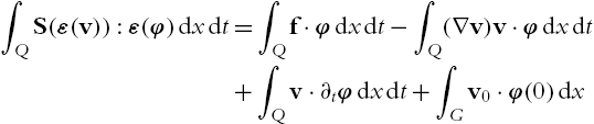
for all φ∈C∞0,div([0,T)×G)![]() with S given by (7.0.2). In this case it follows from parabolic interpolation that (∇v)v⋅v∈L1(Q)
with S given by (7.0.2). In this case it follows from parabolic interpolation that (∇v)v⋅v∈L1(Q)![]() . So the solution is also a test-function and the existence proof is based on monotone operator theory and compactness arguments. These results have been improved by Wolf to the case p>2d+2d+2
. So the solution is also a test-function and the existence proof is based on monotone operator theory and compactness arguments. These results have been improved by Wolf to the case p>2d+2d+2![]() via L∞
via L∞![]() -truncation. Wolf's result was improved to p>2dd+2
-truncation. Wolf's result was improved to p>2dd+2![]() in [65] by the Lipschitz truncation method. Under this restriction on p we have v⊗v∈L1(Q)
in [65] by the Lipschitz truncation method. Under this restriction on p we have v⊗v∈L1(Q)![]() . Hence we can test by Lipschitz continuous functions. So we have to approximate v by a Lipschitz continuous function vλ
. Hence we can test by Lipschitz continuous functions. So we have to approximate v by a Lipschitz continuous function vλ![]() which is quite challenging in the parabolic situation. For further historical comments we refer to Section 5.3.
which is quite challenging in the parabolic situation. For further historical comments we refer to Section 5.3.
We will revise the existence proof from [65]. Using the solenoidal Lipschitz truncation constructed in section 6.1 we can completely avoid the appearance of the pressure and therefore highly simplify the method. For simplicity we only consider the case d=3![]() but all results of this chapter extend to the general case. The main result is as follows.
but all results of this chapter extend to the general case. The main result is as follows.
Theorem 7.0.27

Remark 7.0.12
It is still open whether there exists a weak solution in the case 1<p⩽65![]() . Unlike the stationary case the convective term v⊗v
. Unlike the stationary case the convective term v⊗v![]() is always well-defined independent of the dimension. However, it is not clear how to obtain the compactness of the approximated velocity vm
is always well-defined independent of the dimension. However, it is not clear how to obtain the compactness of the approximated velocity vm![]() in L2(Q)
in L2(Q)![]() . This seems to be necessary to identify the limit of vm⊗vm
. This seems to be necessary to identify the limit of vm⊗vm![]() with v⊗v
with v⊗v![]() .
.
In the next section we show the existence of weak solutions to (7.0.3) in case p>115![]() . Due to this bound on q the space of test functions coincides with the space where the solution is constructed and the convective term becomes a compact perturbation. The result of Section 7.1 will later be used to obtain an approximate solution in the proof of Theorem 7.0.27, see Section 7.2.
. Due to this bound on q the space of test functions coincides with the space where the solution is constructed and the convective term becomes a compact perturbation. The result of Section 7.1 will later be used to obtain an approximate solution in the proof of Theorem 7.0.27, see Section 7.2.
7.1 The approximated system
Throughout this section we assume that S∈C0(Rd×dsym)∩C1(Rd×dsym∖{0})![]() and for some κ⩾0
and for some κ⩾0![]()
λ(κ+|ε|)q−2|σ|2⩽DS(ε)(σ,σ)⩽Λ(κ+|ε|)q−2|σ|2
for all ε,σ∈Rd×dsym∖{0}![]() with some positive constants λ,Λ
with some positive constants λ,Λ![]() .
.
Theorem 7.1.28
Assume (7.1.4) with q>115![]() , f∈Lq′(Q)
, f∈Lq′(Q)![]() and v0∈L2(G)
and v0∈L2(G)![]() . Then there is a solution v∈L∞(0,T;L2(G))∩Lq(0,T;W1,q0,div(G))
. Then there is a solution v∈L∞(0,T;L2(G))∩Lq(0,T;W1,q0,div(G))![]() to
to
∫QS(ε(v)):ε(φ)dxdt=∫Qf⋅φdxdt+∫Qv⊗v:ε(φ)dxdt+∫Qv⋅∂tφdxdt+∫Gv0⋅φ(0)dx
for all φ∈C∞0,div([0,T)×G)![]() .
.
Proof
We mainly follow the ideas of [111], chapter 5. We separate space and time and approximate the corresponding Sobolev space by a finite dimensional subspace. From [111] we infer the existence of a sequence (λk)⊂R![]() and a sequence of functions (wk)⊂Wl,20,div(G)
and a sequence of functions (wk)⊂Wl,20,div(G)![]() , l∈N
, l∈N![]() , such that
, such that
i) wk![]() is an eigenvector to the eigenvalue λk
is an eigenvector to the eigenvalue λk![]() of the Stokes-operator in the sense that
of the Stokes-operator in the sense that
〈wk,φ〉Wl,20=λk∫Gwk⋅φdxfor allφ∈Wl,20,div(G),

ii) ∫Gwkwmdx=δkm![]() for all k,m∈N
for all k,m∈N![]() ,
,
iii) 1⩽λ1⩽λ2⩽...![]() and λk→∞
and λk→∞![]() ,
,
iv) 〈wk√λk,wm√λm〉Wl,20=δkm![]() for all k,m∈N
for all k,m∈N![]() ,
,
v) (wk)![]() is a basis of Wl,20,div(G)
is a basis of Wl,20,div(G)![]() .
.
We choose l>1+d2![]() so that Wl,20(G)↪W1,∞(G)
so that Wl,20(G)↪W1,∞(G)![]() . We are looking for an approximate solution vN
. We are looking for an approximate solution vN![]() of the form
of the form
vN=N∑k=1ckNwk

where CN=(ckN)Nk=1:(0,T)→RN![]() . We will construct CN
. We will construct CN![]() so that vN
so that vN![]() is a solution to
is a solution to
∫GS(ε(vN)):ε(wk)dx=−∫G∂tvN⋅wkdx+∫GvN⊗vN:ε(wk)dx+∫Gf⋅wkdx,k=1,...,NvN(0,⋅)=PNv0.

Here PN![]() is the L2(G)
is the L2(G)![]() -orthogonal projection into XN:=span{w1,...,wN}
-orthogonal projection into XN:=span{w1,...,wN}![]() , i.e.
, i.e.
PN(u):=N∑k=1(∫Gwk⋅udx)wk.

On account of the properties of (wk)![]() equation (7.1.6) is equivalent to
equation (7.1.6) is equivalent to
dckNdt=−∫GS(CN⋅ε(wN)):ε(wk)dx+∑l,jclNcjN∫Gwl⊗wj:∇wkdx+∫Gf⋅wkdx,k=1,...,NckN(0)=∫Gwk⋅v0dx,k=1,...,N.

Since the right-hand-side is not globally Lipschitz continuous in CN![]() the Picard–Lindelöff Theorem only gives a local solution which does not suffice for our purpose. The following lemma helps (see [143], chapter 30).
the Picard–Lindelöff Theorem only gives a local solution which does not suffice for our purpose. The following lemma helps (see [143], chapter 30).
Lemma 7.1.1
So we need to show boundedness of CN![]() in t (assuming its existence). Therefore we multiply the k-th equation of (7.1.6) by ckN
in t (assuming its existence). Therefore we multiply the k-th equation of (7.1.6) by ckN![]() and sum with respect to k. Using ∫GvN⊗vN:∇vNdx
and sum with respect to k. Using ∫GvN⊗vN:∇vNdx![]() we obtain
we obtain
12ddt∫G|vN|2dx+∫G|∇vN|qdx=∫Gf⋅vNdx.

Integration over [0,s]![]() with 0<s⩽T
with 0<s⩽T![]() implies for all κ>0
implies for all κ>0![]()
12∫G|vN(s,⋅)|2dx+λ∫Qs(|∇vN|q−1)dx⩽∫Qsf⋅vNdxdt⩽c(κ)∫Qs|f|q′dxdt+κ∫s0∫G|vN|qdxdt⩽c(κ)∫Qs|f|q′dxdt+κ∫s0∫G|∇vN|qdxdt,

where we used the inequalities of Korn, Young and Poincaré as well as (7.1.4). Choosing κ small enough leads to
supt∈(0,T)∫G|vN(t,⋅)|2dx+∫Q|∇vN|qdxdt⩽c∫Q(|f|q′+1)dxdt

which also implies (7.1.8). Lemma 7.1.1 shows the existence of a solution vN![]() to (7.1.6). Moreover we established with (7.1.9) a useful a priori estimate. Passing to a subsequence implies
to (7.1.6). Moreover we established with (7.1.9) a useful a priori estimate. Passing to a subsequence implies
vN⇀:vinLq(0,T;W1,q0,div(G)),
vN⇀⁎vinL∞(0,T;L2(G)).
In order to pass to the limit in the convective term we need compactness of vN![]() . We obtain from (7.1.6)
. We obtain from (7.1.6)
∫G∂tvN⋅φdx=∫G∂tvN⋅PlNφdx=−∫GS(ε(vN)):ε(PlNφ)dx+∫GvN⊗vN:ε(PlNφ)dx+∫GF:∇PlNφdx=:∫GHN:∇PlNφdx

for all φ∈Wl,20,div(G)![]() (setting F:=∇Δ−1f
(setting F:=∇Δ−1f![]() ). Here PlN
). Here PlN![]() denotes the orthogonal projection into XN
denotes the orthogonal projection into XN![]() with respect to the Wl,20(G)
with respect to the Wl,20(G)![]() inner product. We have uniformly in N
inner product. We have uniformly in N
HN∈Lq0(Q),q0=:min{56q,q′}>1,
as a consequence of (7.1.9), (7.1.4) and F∈Lq′(Q)![]() (which follows from f∈Lq′(Q)
(which follows from f∈Lq′(Q)![]() ). On account of (7.1.12) and Sobolev's embedding (recall the choice of l) we obtain
). On account of (7.1.12) and Sobolev's embedding (recall the choice of l) we obtain
‖∂tvN‖Lq0(0,T;W−l,2div(G))=‖∂tvN‖Lq′0(0,T;Wl,20,div(G))′=sup‖φ‖Lq′0(0,T;Wl,20,div(G))⩽1∫T0∫G∂tvN⋅φdxdt=sup‖φ‖Lq′0(0,T;Wl,20,div(G))⩽1∫T0∫GHN:∇PlNφdxdt⩽sup‖φ‖Lq′0(0,T;Wl,20,div(G))⩽1(∫Q|HN|q0dxdt)1q0(∫Q|∇PNlφ|q′0dxdt)1q′0

and finally
‖∂tvN‖Lq0(0,T;W−l,2div(G))⩽csup‖φ‖Lq′0(0,T;Wl,20,div(G))⩽1‖∇PlNφ‖Lq0(0,T;L∞(G))⩽csup‖φ‖Lq′0(0,T;Wl,20,div(G))⩽1‖PlNφ‖Lq0(0,T;Wl,20,div(G))⩽c.

Combining (7.1.9) and (7.1.13) with the Aubin–Lions compactness Theorem (see Theorem 5.1.23) shows vN→v![]() in L2(0,T;L2div(G))
in L2(0,T;L2div(G))![]() (recall that q>115
(recall that q>115![]() ). This and a parabolic interpolation imply
). This and a parabolic interpolation imply
vN⊗vN→v⊗vinLs(Q)
for all s<56p![]() . Due to (7.1.9) and (7.1.4) we know that S(ε(vN))
. Due to (7.1.9) and (7.1.4) we know that S(ε(vN))![]() is bounded in Lq′(G)
is bounded in Lq′(G)![]() thus
thus
S(ε(vN))⇀˜SinLq′(Q).
Passing to the limit in (7.1.6) leads to
∫Q˜S:ε(φ)dxdt=∫Qf⋅φdxdt+∫Qv⊗v:ε(φ)dxdt+∫Qv⋅∂tφdxdt+∫Gv0⋅φ(0)dx

for all φ∈C∞0,div([0,T)×G)![]() . Note that the class of test-functions which factorize in space and time is dense, see Lemma 5.1.2. In (7.1.16) we also used (for k∈N
. Note that the class of test-functions which factorize in space and time is dense, see Lemma 5.1.2. In (7.1.16) we also used (for k∈N![]() and g∈C∞0[0,T)
and g∈C∞0[0,T)![]() )
)
∫Q∂tvN⋅gwkdxdt=−∫GPNv0⋅wkdxg(0)−∫T0∫GvN⋅wk∂tgdxdt

and PNv0→v0![]() in L2(G)
in L2(G)![]() .
.
Finally we need to show that
˜S=S(ε(v))
holds. We first investigate the time derivative of v. On account of q>115![]() the mapping
the mapping
φ↦∫Qv⊗v:ε(φ)dxdt
belongs to Lq′(0,T;W−1,q′div(G))![]() . The same is true for
. The same is true for
φ↦∫Q˜S:ε(φ)dxdt,φ↦∫Qf⋅φdxdt.

Thus we have ∂tv∈Lq′(0,T;W−1,q′div(G))![]() by (7.1.16) and
by (7.1.16) and
∫Q˜S:ε(φ)dxdt=∫Qf⋅φdxdt+∫Qv⊗v:ε(φ)dxdt−∫T0〈∂tv,v〉dt

for all φ∈Lq(0,T;W1,q0,div(G))![]() . Especially v is an admissible test function. We claim that
. Especially v is an admissible test function. We claim that
v∈Cw([0,T];L2(G)).
Hence we have v(0)=v0![]() and v(t)
and v(t)![]() is uniquely determined for every t∈[0,T]
is uniquely determined for every t∈[0,T]![]() . Sobolev's Theorem for Bochner spaces leads to
. Sobolev's Theorem for Bochner spaces leads to
v∈C([0,T];W−1,q′div(G)).
Let (tn)⊂[0,T]![]() for which tn→t0
for which tn→t0![]() and v(tn,⋅)∈L2(G)
and v(tn,⋅)∈L2(G)![]() for all n∈N
for all n∈N![]() . Then v(tn,⋅)
. Then v(tn,⋅)![]() is bounded in L2(G)
is bounded in L2(G)![]() by (7.1.9) thus
by (7.1.9) thus
v(tn,⋅)⇀:winL2(G).
We have as a consequence of (7.1.20)
v(tn,⋅)→v(t0,⋅)inW−1,q′0(G).
This leads to w=v(t0,⋅)![]() and (7.1.21) implies (7.1.19).
and (7.1.21) implies (7.1.19).
We apply monotone operator theory to show (7.1.17). On account of
∫Q(S(ε(vN))−S(ε(v))):ε(vN−v)dxdt=∫Q(˜S−S(ε(vN))):ε(v)dxdt−∫QS(ε(v)):ε(vN−v)dxdt+∫Q(S(ε(vN)):ε(vN)dxdt−∫Q˜S:ε(v)dxdt
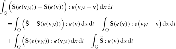
we obtain from (7.1.10) and (7.1.15)
∫Q(˜S−S(ε(vN))):ε(v)dxdt⟶0,N→∞,∫QS(ε(v)):ε(vN−v)dxdt⟶0,N→∞.

Due to (7.1.6) and (7.1.18) we have
∫Q(S(ε(vN)):ε(vN)dxdt−∫Q˜S:ε(v)dxdt=∫Qf⋅(vN−v)dxdt+∫Q(vN⊗vN:ε(vN)−v⊗v:ε(v))dxdt−∫Q∂tvN⋅vNdxdt+∫T0〈∂tv,v〉dt=:(I)+(II)+(III).

We deduce from (7.1.10), (7.1.14) and (7.1.15) that
limN→∞(I)=limN→∞(II)=0.
For the integral involving the convective term we used the assumption q>115![]() . Finally, we obtain
. Finally, we obtain
(III)=12∫G|vN(0)|2dx−12∫G|v(0)|2dx+12∫G|v(T)|2dx−12∫G|vN(T)|2dx=−12∫G|vN(T)−v(T)|2dx−∫GvN(T)⋅v(T)dx+∫G|v(T)|2dx+12∫G|PNv0|2dx−12∫G|v0|2dx.
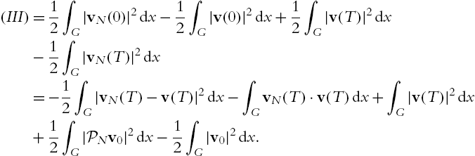
We infer from (7.1.10) and the continuity of PN![]() that limsupN→∞(III)⩽0
that limsupN→∞(III)⩽0![]() (here we took into account (7.1.19) and used vN(T)⇀v(T)
(here we took into account (7.1.19) and used vN(T)⇀v(T)![]() in L2(G)
in L2(G)![]() as a consequence of (7.1.9) and passing to a subsequence) thus
as a consequence of (7.1.9) and passing to a subsequence) thus
∫Q(S(ε(vN))−S(ε(v))):ε(vN−v)dxdt⟶0,N→∞.

Monotonicity of S (which follows from (7.1.4)) implies (7.1.17). □
Corollary 7.1.1
Under the assumptions of Theorem 7.0.27 there is a function ˜π∈C0w([0,T];Lq′0(G))![]() for which
for which
∫QS(ε(v)):ε(φ)dxdt=∫Qf⋅φdxdt+∫Qv⊗v:ε(φ)dxdt+∫Qv⋅∂tφdxdt+∫Gv0φ(0)dx+∫Q˜π∂tdivφdxdt

for all φ∈C∞0([0,T)×G)![]() .
.
Proof
We follow [140], Thm. 2.6. Let φ(t,x)=g(t)ψ(x)![]() with g∈C∞0(0,T)
with g∈C∞0(0,T)![]() and ψ∈C∞0,div(G)
and ψ∈C∞0,div(G)![]() . Setting F:=∇Δ−1f∈Lq′(Q)
. Setting F:=∇Δ−1f∈Lq′(Q)![]() we have
we have
∫Qv⋅ψg′dxdt=∫QS(ε(v)):∇ψgdxdt−∫Qv⊗v:∇ψgdxdt−∫QF:∇ψgdxdt=:−∫QQ:∇ψgdxdt

which is equivalent to
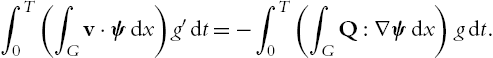
∫T0(∫Gv⋅ψdx)g′dt=−∫T0(∫GQ:∇ψdx)gdt.
If we define
α(t):=∫Gv(t,⋅)⋅ψdx,β(t):=∫GQ:∇ψdx,

we obtain from (7.1.23)
∫T0αg′dt=−∫T0βgdt

for all g∈C∞0(0,T)![]() . Since α and β belong to L1(0,T)
. Since α and β belong to L1(0,T)![]() this implies α′=β
this implies α′=β![]() . Hence the following holds
. Hence the following holds
α(t)=α(0)+∫t0β(s)ds,t∈(0,T).

Now we define
˜Q(t):=∫t0Q(s)ds

and follow from (7.1.25)
∫G((v(t,⋅)−v(0,⋅))⋅ψ+˜Q(t):∇ψ)dx=0

for all ψ∈W1,q0,div(G)![]() . Here we took into account ˜Q(t)∈Lq′(G)
. Here we took into account ˜Q(t)∈Lq′(G)![]() which is a consequence of q>115
which is a consequence of q>115![]() and (7.1.4). De Rahm's Theorem implies the existence of ˜π(t)∈Lq′0(G)
and (7.1.4). De Rahm's Theorem implies the existence of ˜π(t)∈Lq′0(G)![]() for which
for which
∫G((v(t,⋅)−v(0,⋅))⋅ψ+˜Q:∇ψ)dx=∫G˜π(t)divψdx

for all ψ∈W1,q0(G)![]() . For u∈Lq(G)
. For u∈Lq(G)![]() we set ψ=BogG(u−(u)G)∈W1,q0,div(G)
we set ψ=BogG(u−(u)G)∈W1,q0,div(G)![]() so that
so that
∫G˜π(t)udx=∫G˜π(t)(divψ+(u)G)dx=∫G˜π(t)divψdx=∫G((v(t,⋅)−v(0,⋅))⋅ψ+˜Q(t):∇ψ)dx.

Due to v∈Cw([0,T];L2(G))![]() (see (7.1.19)) and ˜Q∈C([0,T];Lq′(G))
(see (7.1.19)) and ˜Q∈C([0,T];Lq′(G))![]() we obtain
we obtain
limt→t0∫G˜π(t)udx=∫G˜π(t0)udx

for all u∈Lq(G)![]() , hence ˜π∈Cw([0,T];Lq′(G))
, hence ˜π∈Cw([0,T];Lq′(G))![]() . Equation (7.1.25) finally implies
. Equation (7.1.25) finally implies
∫QS(ε(v)):∇φdxdt=∫Qv⊗v:∇φdxdt+∫Qf⋅φdxdt+∫Qv⋅∂tφdxdt+∫Gv0⋅φ(0,⋅)dx+∫Q˜π∂tdivφdxdt

for all φ of the class
Y:=span{gψ,g∈C∞0[0,T),ψ∈C∞0(G)}
which is dense (see Lemma 5.1.1). □
Remark 7.1.13
The “original” pressure term π can be obtained by setting π:=∂t˜π![]() . But without further information about the regularity with respect to time of the quantities involved in the equation it only exists in the sense of distributions.
. But without further information about the regularity with respect to time of the quantities involved in the equation it only exists in the sense of distributions.
7.2 Non-stationary flows
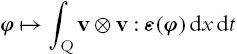
In this section we show how the solenoidal Lipschitz truncation can be used to simplify the existence proof for weak solutions to the power law model for non-Newtonian fluids. We are able to work completely in the pressure free formulation and establish the existence of a solution v∈L∞(0,T;L2(G))∩Lp(0,T;W1,p0,div(G))![]() to
to
∫QS(ε(v)):ε(φ)dxdt=∫Qf⋅φdxdt+∫Qv⊗v:ε(φ)dxdt+∫Qv∂tφdxdt+∫Gv0φ(0)dx

for all φ∈C∞0,div([0,T)×G)![]() .
.
Proof
We start with an approximate system whose solution is known to exist. Let vm∈Lq(0,T;W1,q0,div(G))∩L∞(0,T;L2(G))![]() be a solution to
be a solution to
∫QS(ε(v)):ε(φ)dxdt+1m∫Q|ε(v)|q−2ε(v):ε(φ)dxdt=∫Qf⋅φdxdt+∫Qv⊗v:ε(φ)dxdt+∫Qv∂tφdxdt+∫Gv0φ(0)dx

for all φ∈C∞0,div([0,T)×G)![]() , where q>max{115,p}
, where q>max{115,p}![]() .
.
The existence of vm![]() follows from Theorem 7.1.28. Since we are allowed to test with vm
follows from Theorem 7.1.28. Since we are allowed to test with vm![]() , we find
, we find
12‖vm(t)‖2L2+∫t0∫GS(ε(vm)):ε(vm)dxdσ+1m∫t0∫G|ε(vm)|qdxdσ=12‖v0‖2L2+∫t0∫Gf:vmdxdσ,

for all t∈(0,T)![]() . By coercivity and Korn's inequality we obtain
. By coercivity and Korn's inequality we obtain
∫QS(ε(vm)):ε(vm)dxdt⩾c(∫Q|∇vm|pdxdt−1)

thus
‖m−1/qε(vm)‖q,Q+‖vm‖2L∞(0,T;L2)+‖∇vm‖p,Q⩽c.
Hence we find a function v∈Lp(0,T;W1,p0,div(G))∩L∞(0,T;L2(G))![]() for which (passing to a subsequence)
for which (passing to a subsequence)
∇vm⇀∇vinLp(Q),vm⁎⇀vinL∞(0,T;L2(G)),1m|ε(vm)|q−2ε(vm)→0inLq′(Q).

Since S(ε(vm))![]() is bounded in Lp′(Q)
is bounded in Lp′(Q)![]() by (7.2.30), there exist ˜S∈Lp′(Q)
by (7.2.30), there exist ˜S∈Lp′(Q)![]() with
with
S(ε(vm))⇀˜SinLp′(Q).
Let us have a look at the time derivative. From equation (7.2.28) we get the uniform boundedness of ∂tvm![]() in Lp′(0,T;W−3,2div(G))
in Lp′(0,T;W−3,2div(G))![]() and weak convergence of ∂tvm
and weak convergence of ∂tvm![]() to ∂tv
to ∂tv![]() in the same space (for a subsequence). This shows by using the compactness of the embedding W1,p0,div(G)↪L2σ2div(G)
in the same space (for a subsequence). This shows by using the compactness of the embedding W1,p0,div(G)↪L2σ2div(G)![]() for some σ2>1
for some σ2>1![]() (which follows from our assumption p>65
(which follows from our assumption p>65![]() , resp. p>2nn+2
, resp. p>2nn+2![]() ) and the Aubin–Lions theorem (see Theorem 5.1.23) that vm→v
) and the Aubin–Lions theorem (see Theorem 5.1.23) that vm→v![]() in Lσ(0,T;L2σ2div(G))
in Lσ(0,T;L2σ2div(G))![]() . This and the boundedness in L∞(0,T;L2(G))
. This and the boundedness in L∞(0,T;L2(G))![]() imply that for some σ>1
imply that for some σ>1![]()
vm→vinLs(0,T;L2σ(G))for alls<∞.
As a consequence we have
vm⊗vm→v⊗vinLs(0,T;Lσ(G))for alls<∞.
Overall, we get our limit equation
∫Q˜S:ε(φ)dxdt=∫Qf⋅φdxdt+∫Qv⊗v:ε(φ)dxdt+∫Qv∂tφdxdt+∫Gv0φ(0)dx

for all φ∈C∞0,div([0,T)×G)![]() .
.
The entire forthcoming effort is to prove ˜S=S(ε(v))![]() almost everywhere. We start with the difference of the equation of vm
almost everywhere. We start with the difference of the equation of vm![]() and the limit equation which is
and the limit equation which is
−∫Q(vm−v)⋅∂tφdxdt+∫Q(S(ε(vm))−˜S):∇φdxdt=∫Q(vm⊗vm−v⊗v+m−1|ε(vm)|q−2ε(vm)):∇φdxdt

for all φ∈C∞0,div([0,T)×G)![]() . We define um:=vm−v
. We define um:=vm−v![]() . Then by (7.2.33)
. Then by (7.2.33)
um⇀0inLp(0,T;W1,p0,div(G)),um→0inL2σ(Q),um⇀⁎0inL∞(0,T;L2(G)).

Thus, we can write (7.2.36) as
∫Qum⋅∂tφdxdt=∫QHm:∇φdxdt

for all φ∈C∞0,div(Q)![]() , where Hm:=H1m+H2m
, where Hm:=H1m+H2m![]() with
with
H1m:=S(ε(vm))−˜S,H2m:=vm⊗vm−v⊗v+m−1|ε(vm)|q−2ε(vm).

Moreover, (7.2.31) and (7.2.33) imply
‖H1m‖p′⩽c
as well as
H2m→0inLσ(Q).
Now take any cylinder Q0⋐(0,T)×G![]() . Now, (7.2.37), (7.2.38), (7.2.39) and (7.2.40) ensure that we can apply Corollary 6.1.4. In particular, for suitable ζ∈C∞0(16Q0)
. Now, (7.2.37), (7.2.38), (7.2.39) and (7.2.40) ensure that we can apply Corollary 6.1.4. In particular, for suitable ζ∈C∞0(16Q0)![]() with χ18Q0⩽ζ⩽χ16Q0
with χ18Q0⩽ζ⩽χ16Q0![]() Corollary 6.1.4 implies
Corollary 6.1.4 implies
limsupm→∞|∫(H1m:∇(vm−v))ζχO∁m,kdxdt|⩽c2−k/p.

In other words
limsupm→∞|∫((S(ε(vm))−˜S):∇(vm−v))ζχO∁m,kdxdt|⩽c2−k/p.

Now, the boundedness of S(ε(v))![]() and ˜S
and ˜S![]() in Lp′(16Q0)
in Lp′(16Q0)![]() and Theorem 6.1.25 (h) and (g) give
and Theorem 6.1.25 (h) and (g) give
limsupm→∞|∫((˜S−S(ε(v))):∇(vm−v))ζχO∁m,kdxdt|⩽c2−k/p.

This and the previous estimate imply
limsupm→∞|∫((S(ε(vm))−S(ε(v))):∇(vm−v))ζχO∁m,kdxdt|⩽c2−k/p.

Let θ∈(0,1)![]() . Then by Hölder's inequality and Theorem 6.1.25 (g)
. Then by Hölder's inequality and Theorem 6.1.25 (g)
limsupm→∞∫((S(ε(vm))−S(ε(v))):∇(vm−v))θζχOm,kdxdt⩽c|Om,k|1−θ⩽c2−(1−θ)kp.

This, the previous estimate and Hölder's inequality lead to
limsupm→∞∫((S(ε(vm))−S(ε(v))):∇(vm−v))θζdxdt⩽c2−(1−θ)kp.

For k→∞![]() the right-hand-side converges to zero. Now, the monotonicity of S implies that S(ε(vm))→S(ε(v))
the right-hand-side converges to zero. Now, the monotonicity of S implies that S(ε(vm))→S(ε(v))![]() a.e. in 18Q0
a.e. in 18Q0![]() . This concludes the proof of Theorem 7.0.27. □
. This concludes the proof of Theorem 7.0.27. □
Remark 7.2.14
As done in Corollary 7.1.1 the pressure can be reconstructed. Here we have ˜π∈Lσ(Q)![]() .
.