Chapter 9

Stochastic PDEs

Abstract

In this chapter we revise some well-known tools for SPDEs. In the first section we collect methods from infinite dimensional stochastic analysis, in particular stochastic integration in Hilbert spaces. After this, we give an introduction to the variational approach to SPDEs by considering the stochastic heat equation. Finally, we present the theorems of Prokhorov and Skorokhod which are essential for the stochastic compactness method.

Keywords

Infinite dimensional stochastic analysis; Stochastic PDEs; Stochastic heat equation; Variational approach; Galerkin method; Compactness; Skorokhod's Theorem

9.1 Stochastic analysis in infinite dimensions

In the following we extend the setup from the previous chapter to the case of Banach or Hilbert space valued stochastic processes (see [55]).

Let (V,V)Image be a Banach space and 1p<Image. We denote by Lp(Ω,F,P;V)Image the Banach space of all measurable mappings v:ΩVImage such that

E[vVp]<,

Image

where the expectation is taken with respect to (Ω,F,P)Image. The measurability has to be understood via the approximation by step functions similar to Section 5.1. Regarding the reflexivity and the dual spaces we have the same results as in the case of Bochner spaces (see Lemma 5.1.1). The definitions of adaptivity and progressive measurability (see Chapter 8) extend in a straightforward manner to Banach space valued processes. The definition of the stochastic integral can be extended to Hilbert spaces, where the process X as well as the stochastic integral take values in some Hilbert spaces (H,H)Image. Let U be a Hilbert space with orthonormal basis (ek)kNImage and let L2(U,L2(G))Image be the set of Hilbert–Schmidt operators from U to L2(G)Image. Recall that a bounded linear operator Φ:UL2(G)Image is called Hilbert–Schmidt operator iff

kNΦekL2(G)2<.

Image

We consider a cylindrical Wiener process W=(Wt)t[0,T]Image which has the form

W(σ)=kNekβk(σ)

Image (9.1.1)

with a sequence (βk)kNImage of independent real valued Brownian motions on (Ω,F,P)Image. Define further the auxiliary space U0UImage as

U0:={e=kαkek:kαk2k2<},eU02:=k=1αk2k2,e=kαkek,

Image (9.1.2)

thus the embedding UU0Image is Hilbert–Schmidt and trajectories of W belong PImage-a.s. to the class C([0,T];U0)Image (see [55]).

For ψL2(Ω,F,P;L2(0,T;L2(U,L2(G))))Image progressively (Ft)t0Imagemeasurable we see that the equality

0tψ(σ)dWσ=k=10tψ(σ)(ek)dβk(σ)

Image (9.1.3)

defines a PImage-a.s. continuous L2(G)Image-valued (Ft)t0Image-martingale. Moreover, we can multiply the above with test-functions since

G0tψ(σ)dWσφdx=k=10tGψ(σ)(ek)φdxdβk(σ),φL2(G),

Image

is well-defined and PImage-a.s. continuous.

In the following we define the quadratic variation of a stochastic process with values in a Hilbert space.

Definition 9.1.1

Let (Xt)t[0,T]Image be a continuous semi-martingale on a probability space (Ω,F,P)Image with values in a separable Hilbert space (H,,H)Image with basis (ei)iNImage. Then its quadratic variation process is defined as

X,XtH:=i,jNX,eiH,X,ejHtej,Hei

Image

and has values in N(H)Image (the set of nuclear operators on HImage). Moreover, we define the trace of X,XtHImage by

trX,XtH:=iNX,eiH,X,eiHtei,Hei.

Image

Very useful is also the Burkholder–Davis–Gundi inequality.

Lemma 9.1.1

Let (H,,H)Image be a separable Hilbert space, (Ω,F,P)Image be a probability space and (Xt)t[0,T]Image be a continuous martingale on (Ω,F,P)Image with values in HImage. Then we have for all p>0Image

cpE[supt(0,T)XtH]pE[trX,XTHN(H)]p2CpE[supt(0,T)XtH]p,

Image

where cp,CpImage are positive constants.

Now we present an infinite dimensional version of Itô's formula which is appropriate at least to obtain energy estimates for linear SPDEs, see [105, Theorem 3.1] or [127, Chapter 4.2, Theorem 2].

Theorem 9.1.39

Let (V,V)Image be a Banach space which is continuously embedded into a separable Hilbert space (H,,H)Image. Let (Ω,F,P)Image be a probability space. Assume that the processes (Xt)t[0,T]Image and (Yt)t[0,T]Image, taking values in VImage and VImage, respectively, are progressively measurable and

P{0T(XV2+YV2)dt<}=1.

Image

Assume further that there is a continuous martingale (Mt)t[0,T]Image, taking values in HImage, such that, for P×L1Image-a.e. (ω,t)Image, the following equality holds:

X(t),φH=X(0),φH+0tVY(σ),φVdσ+Mt,φHφV.

Image

Then we have

X(t)H2=X(0)H2+0tVY(σ),X(s)Vdσ+20tX(σ),dMσH+trM,MtHN(H),P×L1-a.e.

Image

In Lemma C.0.1 in Appendix C we will establish a version of Itô's formula which is appropriate for nonlinear PDEs, in particular for stochastic Navier–Stokes equations and problems with polynomial nonlinearities.

In some applications we need fractional time derivatives of stochastic integrals. The following lemma is concerned with fractional derivatives of stochastic integrals in Hilbert spaces (see [73, Lemma 2.1] for a proof).

Lemma 9.1.2

Let ΨLp(Ω,F,P;Lp(0,T;L2(U,L2(G))))Image (p2Image) be progressively (Ft)t0Image-measurable and W a cylindrical (Ft)t0Image-Wiener process as in (9.1.1). Then the following holds for any α(0,1/2)Image

E[0ΨdWσWα,p(0,T;L2(G))p]c(α,p)E[0TΨL2(U,L2(G))pdt].

Image

If we have higher moments it is possible to improve the fractional time differentiability to Hölder-continuity.

Lemma 9.1.3

Let (Ω,F,P)Image be a probability space endowed with the filtration (Ft)t0Image.

a) Let W be a M-dimensional Brownian motion with respect to (Ft)t0Image. Let XLβ(Ω,F,P;Lβ(0,T))Image, β>2Image, be a progressively (Ft)t0Image-measurable process with values in RN×MImage. Then the paths of the process Zt:=0tXdWσImage are PImage-a.s. Hölder continuous with exponent α(1β,12)Image and we have

E[ZCα([0,T])β]cαE[0T|X|βdt].

Image

b) Let ψLβ(Ω,F,P;Lβ(0,T;L2(U,L2(G))))Image, β>2Image, be progressively (Ft)t0Image-measurable and W a cylindrical (Ft)t0Image-Wiener process as in (9.1.1). Then the paths of the process Zt:=0tψdWσImage are PImage-a.s. Hölder continuous with exponent α(1β,12)Image and the following holds

E[ZCα([0,T];L2(G))β]cαE[0TψL2(U,L2(G))βdt].

Image

Proof

a) We follow [94], proof of Lemma 4.6, and consider the Riemann–Liouville operator: let X be a Banach space, p(1,]Image, α(1p,1]Image and fLp(0,T;X)Image. Then the Riemann–Liouville operator is given by

(Rαf)(t):=1Γ(α)0t(tσ)α1f(σ)dσ,t[0,T].

Image

It is well known that RαImage is a bounded linear operator from fLp(0,T;X)Image to Cα1/p([0,T];X)Image (see [130], Thm. 3.6). According to the stochastic Fubini Theorem (see [55], Thm. 4.18) we have Zt=Rα(Z˜t)Image, where

Z˜t=1Γ(1α)0t(tσ)αX(t)dWσ,t[0,T].

Image

For α(1β,12)Image we obtain by the Burkholder–Davis–Gundi inequality and Young's inequality for convolution that

E[ZCα1/β([0,T])β]cE[0T|Z˜(t)|βdt]c0TE[sup[0,t]|Z˜(σ)|]βdtc0TE[0t(tσ)2α|X(σ)|2dσ]β2dtcE[0T|X|βdt].

Image

b) By exactly the same arguments we end up with

E[ZCα1/β([0,T];L2(G))β]cE[0TZ˜(t)L2(G)βdt]c0TE[sup[0,t]Z˜(σ)L2(G)β]βdtc0TE[i0t(tσ)2αψ(ei)L2(G)2dσ]β2dt=c0TE[0t(tσ)2αψ(σ)L2(U,L2(G))2dσ]β2dtcE[0TψL2(U,L2(G))βdt].

Image

This concludes the proof.  □

The following lemma is very useful in order to pass to the limit in stochastic integrals (see [56, Lemma 2.1])

Lemma 9.1.4

Consider a sequence of cylindrical Wiener processes (Wn)Image over U (see (9.1.1)) with respect to the filtration (Ft)t0Image. Assume that (Ψn)Image is a sequence of progressively (Ft)t0Image-measurable processes such that ΨnL2(0,T;L2(U,L2(G)))Image PImage-a.s. Suppose there is a cylindrical (Ft)t0Image-Wiener process W and ΨL2(0,T;L2(U,L2(G)))Image, progressively (Ft)t0Image-measurable, such that

WnWinC0([0,T];U0),ΨnΨinL2(0,T;L2(U,L2(G))),

Image

in probability. Then we have

0ΨndWn0ΨdWinL2(0,T;L2(G)),

Image

in probability.

9.2 Stochastic heat equation

As a preparation for the stochastic models for power law fluids we will study the stochastic heat equation by means of a Galerkin–Ansatz. So we seek for a (Ft)t0Image-adapted process u:Ω×(0,T)×GRImage satisfying

{dut=Δudt+ΦdWt,u(0)=u0.

Image (9.2.4)

Here W is a cylindrical (Ft)t0Image-Wiener process (see (9.1.1)), u0L2(Ω,F0,P;L2(G))Image is some initial datum and Φ is a progressively (Ft)t0Image-measurable process taking values in the space of Hilbert–Schmidt operators. More precisely, we assume

ΦL2(Ω,F,P;L2(0,T;L2(U;L2(G)))).

Image (9.2.5)

Typically one supposes some (nonlinear) dependence of Φ on u. But we neglect this here for simplicity. The Hilbert space U on which W is defined will most naturally be L2(G)Image. As in the case of stochastic ODEs (9.2.4) is an abbreviation for the integral equation

u(t)=u0+0tΔudσ+0tΦdWσ.

Image

The stochastic integral has to be understood as in (9.1.3). The integral 0tΔudσImage makes sense in case of a strong solution, i.e. if ΔuL1((0,T)×G)Image a.s. In order to understand the weak formulation (weak in the PDE-sense) we multiply the above with test-functions φC0(G)Image, thereby obtaining the following equality, which holds PImage-a.s.:

Gu(t)φdx=Gu0φdx0tGuφdxdσ+Gφ(0tΦdWσ)dx

Image (9.2.6)

for a.e. t(0,T)Image. Due to (9.2.5) this can be equivalently formulated using test-functions for W01,2(G)Image. The natural solution space for this is obviously

L2(Ω,F,P;L2(0,T;W01,2(G))).

Image

Theorem 9.2.40

Let (Ω,F,P)Image be a probability space with right-continuous filtration (Ft)t0Image, let u0L2(Ω,F0,P;L2(G))Image and assume that Φ satisfies (9.2.5) and is progressively (Ft)t0Image-measurable. Then there is a progressively (Ft)t0Image-measurable process

uL2(Ω,F,P;L2(0,T;W01,2(G)))

Image

such that (9.2.6) holds. We also have uC([0,T];L2(G))Image a.s. with

E[supt(0,T)G|u(t)|2dx]<.

Image

The solution u is unique in the above class.

Proof

We will split the proof in several steps. First we approximate (9.2.6) by a Galerkin–Ansatz. Then we show a priori estimates and finally we pass to the limit. Note that the uniqueness of solutions is obvious: the difference of two potential solutions solves a deterministic heat equation with zero initial datum.

Step 1: approximation

We will solve (9.2.6) by a finite dimensional approximation. So we need an appropriate basis of W01,2(G)Image. A good choice is the set of eigenfunctions of the Laplace operator. There is a smooth orthonormal system (wk)kNL2(G)Image and (λk)(0,)Image such that

Gwkφdx=λkGwkφdxφW01,2(G).

Image (9.2.7)

We seek the approximate solution uNImage such that

uN=k=1NcNiwk=CNwN,wN=(w1,...,wN),

Image

where CN=(cNi):Ω×(0,T)RNImage. Therefore, we would like to solve the system

GduNwkdx+Gukwkdxdt=GΦdWσNwkdx,k=1,...,N,uN(0)=PNu0.

Image (9.2.8)

Here PN:Ldiv2(G)XN:=span{w1,...,wN}Image is the orthogonal projection, i.e.

PNu=k=1Nu,wkL2wk.

Image

Equation (9.2.8) is to be understood PImage-a.s. and for a.e. t and we assume

WN(σ)=k=1Nekβk(σ)=eNβN(σ).

Image

It is equivalent to solving

{dCN=ΛCNdt+ΣdβtN,CN(0)=C0,

Image (9.2.9)

where Λ,ΣRN×NImage with

Λij=δijλj,Σij=GΦeiwjdx.

Image

As (9.2.9) is a linear system of ODEs we obtain a unique solution (with a.s. continuous trajectories) by the results of Section 8.4.

Step 2: a priori estimates

We apply Itô's formula to the function f(C)=12|C|2Image, thereby obtaining

12uN(t)L2(G)2=12CN(0)L2(G)2+0tCNd(CN)σ+120tI:dCNσ=12PNu0L2(G)20tGuNuNdxdσ+G0tuNΦdWσNdx+12k0tΣkk2dxdσ.

Image (9.2.10)

In the above we used (9.2.7) and

dcNk=GuNwkdxdt+GΦdWtNwkdx,cNi,cNj=k=1N0GΦejwkdxdβk,l=1N0GΦeiwldxdβl=k=1Nl=1N0GΦejwkdxdβk,0GΦeiwldxdβl=k=1N(GΦejwkdx)(GΦeiwkdx)=(Σ2)ij.

Image

Now we obtain, taking the supremum in time and taking expectations, that

E[supt(0,T)G|uN(t)|2dx+0TG|uN|2dxdσ]cE[G|u0|2dx+k=1N0TΣkk2dt+supt(0,T)|J(t)|],

Image

where we set

J(t)=G0tuNΦdWσNdx.

Image

By Hölder's inequality and an account of wk2=1Image, straightforward calculations show

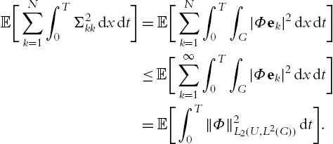
E[k=1N0TΣkk2dxdt]=E[k=1N0TG|Φek|2dxdt]E[k=10TG|Φek|2dxdt]=E[0TΦL2(U,L2(G))2dt].

Image

On account of Burkholder–Davis–Gundi inequality (Lemma 9.1.1) and Young's inequality we obtain

E[supt(0,T)|J(t)|]=E[supt(0,T)|0tGuNΦdxdWσN|]=E[supt(0,T)|0tk=1NGuNΦekdxdβk(σ)|]cE[0Tk=1N(GuNΦekdx)2dt]12cE[(0T(k=1NG|uN|2dxG|Φek|2dx)dt]12cE[supt(0,T)G|uN|2dx(0Tk=1G|Φek|2dxdt)]12δE[supt(0,T)G|uN|2dx]+c(δ)E[0TΦL2(U,L2(G))2dt],

Image

for any arbitrary δ>0Image. If δ is sufficiently small this finally proves

E[supt(0,T)G|uN(t)|2dx+0TG|uN|2dxdσ]cE[G|u0|2dx+0TΦL2(U,L2(G))2dt].

Image (9.2.11)

By our assumptions the right-hand-side is finite.

Step 3: passage to the limit

Due to (9.2.11) and passing to a subsequence we obtain a limit function u:

uNuinL2(Ω,F,P;L2(0,T;W01,2(G))).

Image (9.2.12)

We also have that uL(0,T;L2(G))Image a.s. and

E[supt(0,T)G|u(t)|2dx]<.

Image (9.2.13)

We compute for ψL2(Ω×(0,T))Image and φW01,2(G)Image

E[0TGu(t)ψ(t)φdxdt]=limNE[0TGuN(t)ψ(t)φdxdt]=limNE[0TGuN(t)ψ(t)PNφdxdt]=limNE[0T(GPNu0ψ(t)φdxdt+0tGuNψ(t)φdxdσ+G0tψPNφΦdWσNdx)].

Image

We have to pass to the limit in all terms. The first integral converges as PNwwImage in L2(G)Image for any wL2(G)Image. The second term converges because of (9.2.12). Finally, we use

WNWinL2(Ω,F,P;C([0,T];U0)),

Image

for the stochastic integral (recall Lemma 9.1.4). All together we obtain

E[0TGu(t)ψ(t)φdxdt]=E[0TG(u0ψ(t)φ+0tψ(t)φdσ+0tψφΦdWσ)dx],

Image

which implies that PImage-a.s.

Gu(t)φdx=Gu0φdx0tGuφdxdσ+Gφ(0tΦdWσ)dx

Image

as ψ was arbitrary.

Step 4: continuity of u

Interpreted as an element of W1,2(G)Image we can write PImage-a.s.

u(t)=0tΔudσ+0tΦdWσ

Image

for a.e. t. For any α<12Image the deterministic integral belongs PImage-a.s. to the class

W1,2(0,T;W1,2(G))Cα([0,T];W1,2(G)).

Image

For the stochastic integral we have

0ΦdWσC([0,T];(L2(G)))C([0,T];W1,2(G))P-a.s.

Image

This follows from the construction and our assumption (9.2.5). Combining both facts shows that uC([0,T];W1,2(G))Image. This and (9.2.11) yields

uCw([0,T];L2(G))P-a.s.

Image (9.2.14)

We want to strengthen (9.2.14) and obtain continuity with respect to the norm topology. We apply Itô's formula in infinite dimensions, Theorem 9.1.39, with H=L2(G)Image, V=W01,2(G)Image, X=uImage, Y=Vu,VImage and M=0ΦdWσImage. We have

G|u(t)|2dx=G|u(0)|2dx0tG|u|2dxdσ+2G0tuΦdWσdx+0tΦL2(U,L2(G))2dt.

Image

As the right-hand-side is continuous so is the left-hand-side, i.e.

[0,T]tG|u(t)|2dx

Image

is PImage-a.s. continuous. This and (9.2.14) implies uC([0,T];L2(G))Image a.s.  □

9.3 Tools for compactness

In this section we present some (mainly basic) tools from probability theory which are quite crucial to obtain compactness for SPDE. Let (V,τ)Image be a topological space. The smallest σ-field B(V)Image on (V,τ)Image which contains all open sets is called topological σ-field. A random variable with values in the topological space (V,τ)Image is a measurable map X:(Ω,F)(V,B(V))Image. The probability law μ of X on (V,τ)Image will be given by μ=PX1Image. An important concept for applications is the pre-compactness of families of random variables. We will need the following definition.

Definition 9.3.1

Tightness

A family (μα)αIImage of probability laws on a topological space (V,B(V))Image is called tight if for every ε>0Image there is a compact subset KVImage such that μα(K)1εImage for every αIImage.

Lemma 9.3.1

Prokhorov; [96], Thm. 2.6

Let (μα)αIImage be a family of probability laws on a metric space (V,ρ)Image. If (μα)αIImage is tight then it is also relatively compact.

Lemma 9.3.2

Skorokhod; [96], Thm. 2.7

Let (μn)nNImage be a sequence of probability laws on a complete separable metric space (V,ρ)Image such that μnμImage weakly in the sense of measures as nImage. Then there is a probability space (Ω_,F_,P_)Image and random variables (X_n)nN,X_:(Ω_,F_,P_)(V,B(V))Image such that:

• The laws of X_nImage and X_Image under P_Image coincide with μnImage and μ respectively, nNImage.

• We have P_Image a.s. that X_nρX_Image for nImage.

The proof of Lemma 9.3.2 in the general case is not very long but quite technical and it is hard to grasp the main ideas. We will therefore briefly outline the case of real-valued random variables, i.e. V=RImage and ρ(x,y)=|xy|Image. Let μnImage be a probability law on RImage such that μnμImage weakly in the sense of measures as nImage. We denote by FnImage and F the distribution functions of μnImage and μ respectively. Let us assume for simplicity that they are injective (otherwise one can argue via their generalized inverse functions). In this case we have FnFImage pointwise. Now we set (Ω_,F_,P_)=((0,1),B((0,1)),L1|(0,1))Image. Let us assume for simplicity that the distribution functions FnImage (nNImage) and F are continuous. We define random variables (for ω(0,1)Image)

X_n(ω)=Fn1(ω),X_(ω)=F1(ω).

Image

Now one can easily see that for nNImage

μX_n=P_X_n1=L1Fn=μn

Image

and similarly μX_=μImage. Moreover, we have

X_n(ω)=Fn1(ω)F1(ω)=X_(ω)

Image

for every ω(0,1)Image. In the general case this convergence only holds true in points where X_Image is continuous (which is in L1Image-a.e. ω).

Lemma 9.3.2 only applies to metric spaces. Unfortunately, this does not cover Banach spaces with the weak topology. Therefore we need the following generalization.

Definition 9.3.2

Quasi-Polish space

Let (V,τ)Image be a topological space such that there exists a countable family

{fn:V[1,1];nN}

Image

of continuous functions that separates points of VImage. Then (V,τ,(fn)nN)Image is called a quasi-Polish space.

Lemma 9.3.3

Jakubowski–Skorokhod, [99]

Let (μn)nNImage be a family of probability laws on a quasi-Polish space (V,τ,(fn)nN)Image and let SImage be the σ-algebra generated by the maps (fn)nNImage. Let (μn)nNImage be a tight sequence of probability laws on (V,S)Image. Then there is a subsequence (μnk)kNImage such that the following holds. There is a probability space (Ω_,F_,P_)Image and random variables (X_k)kN,X_:(Ω_,F_,P_)(V,S)Image such that:

• The laws of X_kImage under P_Image coincide with μnkImage, kNImage.

• We have P_Image-a.s. that X_kτX_Image for kImage.

• The law of X_Image under P_Image is a Radon measure.

References

[55] G. Da Prato, J. Zabczyk, Stochastic Equations in Infinite Dimensions. Encycl. Math. Appl.. Cambridge: Cambridge University Press; 1992;vol. 44.

[56] A. Debussche, N. Glatt-Holtz, R. Temam, Local martingale and pathwise solutions for an abstract fluids model, Phys. D, Nonlinear Phenom. 2011;240(14–15):1123–1144.

[73] F. Flandoli, D. Ga̧tarek, Martingale and stationary solutions for stochastic Navier–Stokes equations, Probab. Theory Relat. Fields 1995;102:367–391.

[94] M. Hofmanová, Degenerate parabolic stochastic partial differential equations, Stoch. Process. Appl. 2013;123(12):4294–4336.

[96] N. Ikeda, S. Watanabe, Stochastic Differential Equations and Diffusion Processes. 2nd ed. N.-Holl. Math. Libr.. Amsterdam: North-Holland; 1989;vol. 24.

[99] A. Jakubowski, The almost sure Skorokhod representation for subsequences in nonmetric spaces, Teor. Veroâtn. Primen. 1997/1998;42(1):209–216. translation in Theory Probab. Appl. 1998;42(1):167–174.

[105] N.V. Krylov, B.L. Rozovskii, Stochastic evolution equations. Itogi Nauki i Tekh. Ser. Sovrem. Probl. Mat.. Moscow: VINITI; 1979;vol. 14:71–146. English transl.: J. Sov. Math. 1981;16(4):1233–1277.

[127] B.L. Rozovskii, Stochastic evolution systems. Linear theory and applications to non-linear filtering. Math. Appl., Sov. Ser.. Dordrecht etc.: Kluwer Academic Publishers; 1990;vol. 35 xviii.

[130] S.S. Samko, A.A. Kilbas, O.I. Marichev, Fractional Integrals and Derivatives. Yverdon: Gordon and Breach; 1993.

..................Content has been hidden....................

You can't read the all page of ebook, please click here login for view all page.
Reset
13.58.51.228