Chapter 5. Calculation of Properties
So far we have encountered several thermodynamic properties: molar volume, internal energy, enthalpy, entropy, heat capacities. They are all state functions, meaning that they are fixed once the state is fixed. An immediate consequence of practical importance is that thermodynamic properties can be tabulated once and for all. Tabulations have their limitations, however. Tables are impractical for mass-calculations such as those involved in large scale design, and of course it is impractical to tabulate properties of all conceivable substances under all conceivable states. Thus the need to develop methodologies for the numerical calculation of thermodynamic properties. In this chapter we have two main goals: (a) to develop relationships among the various thermodynamic properties and (b) to develop methodologies for the calculation of enthalpy and entropy as a function of pressure and temperature. Our focus continues to be on pure fluids. The extension to multicomponent systems is discussed in Chapter 9.
Instructional Objectives. In this chapter we will learn how to:
1. Manipulate the differential of thermodynamic properties.
2. Generate relationships between properties.
3. Calculate properties using the equation of state.
4. Properly apply reference states in the calculation of absolute properties.
This chapter makes extensive use of calculus. The most important concepts are reviewed here, but for more details you should consult a dedicated textbook.
5.1 Calculus of Thermodynamics
In dealing with pure substances we have two independent variables. Though we prefer to choose pressure and temperature, any two variables from the set {V, P, T, S, H, ···} may be used for this purpose.1 The same thermodynamic property may be written in various equivalent forms, depending on the pair that is chosen as the independent variables. This leads to a large number of relationships among the many properties. This is a good thing because it provides us with many alternative ways to perform a given calculation. It can also be a source of confusion if we lose track of the logic that governs these relationships and treat them instead as equations to be memorized. This logic is provided by the tools of multivariate calculus. In preparation for this discussion we first review some useful mathematical tools.
1. For example, in the PV graph we have chosen P and V as the independent variables. Isotherms and isobars on that graph are expressed functions of H and S.
Thermodynamic properties are state functions. Mathematically,
F = F(X, Y),
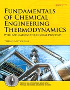
which states that property F has a fixed value once the independent state variables X and Y are fixed. The differential of this function is given by
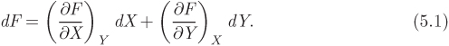
A useful mathematical property is the triple-product rule. We set F = const., from which dF = 0. The differential then becomes
The last result is written more formally as
or, equivalently,
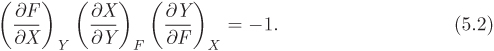
This relationship exists between any three variables that are related by an equation. Since volume, pressure, and temperature are related via the equation of state, we obtain the following result as an immediate consequence of the triple-product rule:

The symmetry between F, X, and Y in the triple-product rule indicates that it does not matter which variable is taken to be the function and which are the independent variables since the equation F = F(X, Y) can be solved to give X as a function of F and Y, or Y as a function of F and X.


f(x1, y1) − f(x0, y0).
Exact Differential The differential of a function F(X, Y) has the general form
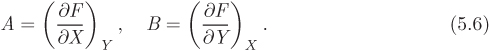
where A and B are functions of X and Y and represent the partial derivatives of F:
We also have the following relationship between A and B
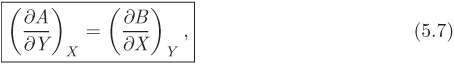
which expresses the fact that the mixed derivative of F does not depend on the order of differentiation:

While the differential of any function F(X, Y) is always of the form in eq. (5.5), the opposite is not true: not every expression of the form in eq. (5.5) represents the differential of a function F(X, Y), unless the two relationships in eq. (5.6) is also satisfied. If these relationships are indeed satisfied, then A and B are identified as the partial derivatives of F(X, Y). As a further consequence, the integration of dF between two points depends only on the coordinates of the initial and final points and is independent of the integration path. Such differential is called exact. If eq. (5.7) is not satisfied, the differential is inexact. As a consequence, its integration produces different results depending in the path. This is another way of saying that if dF is an inexact differential, F cannot be represented by a function F(X, Y), as such function integrated between (X1, Y1) and (X2, Y2) would produce F(X2, Y2) − F(X1, Y1), regardless of the path.
The relevance to thermodynamics is this: thermodynamic properties are state functions and their differential with respect to any set of independent variables is exact. On the other hand, heat and work are path functions and their differentials are inexact. Our goal in this chapter is to develop differential expressions for enthalpy and entropy. These differentials will be of the form in eq. (5.5). Once we have the differential form of a property, we will be able to calculate changes between any two states by straightforward integration.
Note
Calculus and Thermodynamics
There is a correspondence between thermodynamic language and mathematics:
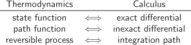
The corresponding terms in this table are equivalent; in other words, they mean the same thing.
5.2 Integration of Differentials
A recurring problem in thermodynamics is the calculation of the change of a property F between two states (X1, Y1) and (X2, Y2). To perform this calculation, we devise a reversible path between the end states and consider a small step during which the state changes by (dX, dY). The corresponding change in F is given by its differential
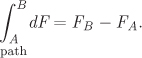
To calculate the change ΔFAB for a change of state from A to B we integrate this differential from the initial state to the final state:
As we saw in Example 5.3, such integration requires the specification of a path, namely, an equation that relates the independent variables as they change from the initial to the final state. Nonetheless, the result of the integration must be equal to the difference between the value of F at the initial and final state,
Therefore, while a path is necessary to perform the integration, the result is independent of the path. This is true for all thermodynamic properties and has a very practical implication: to calculate the change of a thermodynamic property between two states we are free to choose the integration path any way we want. It makes sense then to pick a path that makes the calculation easier.
The geometric interpretation of this integration is shown in Figure 5-1. The independent variables are shown as axes on the horizontal plane and F is shown on the vertical axis. The state of the system is represented by a point on the XY plane. Function F is represented by a surface, which for simplicity is not shown. Integration is equivalent to calculating dF for small changes of state along the integration path and adding up all contributions. By the time the final state is reached, the integral must be equal to the difference FB − FA. Clearly, any path must yield the same value of the integral. Mathematically convenient paths are those that consist of segments in which one variable is held constant. Path AB′B consists of a constant-X portion (AB′) followed by a constant-Y part (B′B). In the constant-X part, dX = 0, thus only the Y-derivative is integrated. Similarly, along the constant-Y portion we have dY = 0, and the only derivative that is integrated is the one with respect to X. Such paths correspond to elementary processes, for example, isothermal isentropic, which correspond to constant temperature, constant entropy, and so on. For this reason, elementary processes are useful not only as experimental tools, but also as mathematical paths for the integration of thermodynamic differentials.
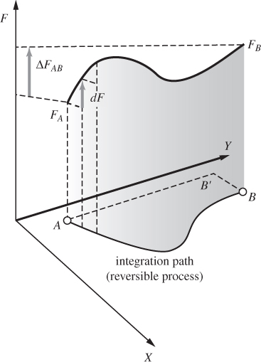
Figure 5-1: Geometric interpretation of the integration path. As the state traces the integration path on the XY plane, property F traces a line on the F (X, Y) surface.
5.3 Fundamental Relationships
The Maxwell relationships are a set of relationships among various partial derivatives involving the following properties: T, S, P, and V. These, as well as additional relationships, can be obtained in a systematic and straightforward way. We begin by considering a closed system undergoing a reversible process without any shaft work. The system may exchange heat and PV work with the surroundings. We focus on a small step along the path. By first law,
For a reversible process, the PV work is −PdV, and the second law gives dQ = TdS. We make these substitutions into the first law to obtain the first important equation:
This equation is of fundamental importance. Its thermodynamic interpretation is that it gives the change in internal energy as a result of a small change of state under reversible conditions. Its mathematical interpretation is that it expresses the differential of the internal energy, using entropy and volume as the independent variables. Internal energy is a state function, therefore, the above is an exact differential. As an immediate consequence we recognize the multipliers of dS and dV as partial derivatives of U (see eqs. [5.5] and [5.6]):
A second result follows by applying the criterion of the exact differential, eq. (5.7), to these derivatives:
Analogous relationships can be obtained for enthalpy. Beginning with the definition H = U + PV, the differential of H is dH = dU + PdV + VdP. Substituting eq. (5.11) for dU we obtain
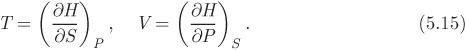
This is also of the form in eq. (5.5) and gives the differential of enthalpy with entropy and pressure as the independent variables. Now we identify the multipliers of dS and dP as the following partial derivatives:
An additional relationship is obtained by applying the criterion of exactness:

We apply the same procedure to the Gibbs free energy, G = H − TS, whose differential is dG = dH − TdS − SdT. Using eq. (5.14), this becomes
Following eq. (5.6) we make the identifications:
Applying the criterion of exactness we obtain,
A final set of relationships is obtained for the Helmholtz free energy, A = U − TS. Its differential is dA = dU − TdS − SdT, and this, using eq. (5.11), becomes
We identify the partial derivatives,
and obtain the following result by virtue of the exactness criterion:
With this we have completed the derivations of this section.
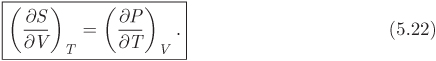
All of these results are exact relationships among various properties. They are general and apply to any pure substance,2 whether gas, liquid, or solid. All other relationships in thermodynamics may be considered as mathematical consequences of the results obtained here. Equations (5.13), (5.16), (5.19), and (5.22) are known as the Maxwell relationships. They relate various partial derivatives among the set of the four fundamental variables, P, V, T, and S, and they are very useful when we want to change from one set of independent variables to another. The complete results of these sections are summarized in Table 5-1.
2. More specifically, these results apply to any closed system of constant composition, for example, any mixture undergoing changes of state as long as its composition does not change (through chemical reaction, for example).
Table 5-1: Summary of fundamental relationships

There is a certain symmetry between these results: properties U, H, G, and A, all of which have units of energy, or energy per mass3 appear as the dependent variables; properties P, V, T, and S, appear as independent variables in combinations that involve dP or dV, and dT or dS. Many more such relationships can be obtained. If the differential of dU is solved for dS, we obtain the differential of entropy in terms of U and V:
3. We have written these equations in intensive form, such as for a unit of mass (1 mol or 1 kg) undergoing a change of state. All equations in Table 5-1 can be written for the extensive form of the properties involved, corresponding to mass m, or n number of moles.
This too is an exact differential and can be used to produce additional set of relationships.4 This procedure may be repeated with other properties as well. All these equations are a consequence of the fact that we have a wide choice for the pair of variables that we take to be independent. Mathematically, these derivations are an exercise in changing variables.
4. Some of the results obtained in this manner will be redundant with the ones obtained already.
5.4 Equations for Enthalpy and Entropy
The stated goal for this chapter is to obtain equations for the enthalpy and entropy in terms of pressure and temperature.5 We approach this as a calculus problem: if enthalpy is taken to be a function of T and P, the general form of its differential must be,
5. Equation (5.14) is not useful in this respect because the independent variables are entropy and pressure, rather than temperature and pressure.
We recognize the partial derivative with respect to temperature as the constant-pressure heat capacity. The derivative with respect to pressure was calculated in eq. (5.23). Combining these results,
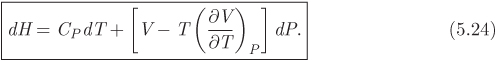
This is the desired equation and gives the differential of enthalpy with pressure and temperature as the independent variables. To obtain an analogous equation for entropy, we start with eq. (5.14), which we solve for dS:
Using eq. (5.24) for dH we obtain
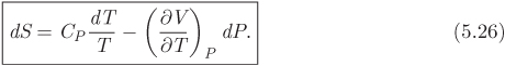
Equations (5.24) and (5.26) are important results: not only do they express enthalpy and entropy in terms of pressure and temperature, but their computation requires only the equation of state, which is needed to calculate the factor of the pressure term, and the heat capacity. Therefore, the calculation of enthalpy and entropy is reduced to the selection of a suitable equation of state. In the remainder of this chapter we will produce alternative forms of these equations, suitable for calculation with cubic equations of state. First, however, we point out that as an immediate consequence of these equations, we obtain simple expressions for the special case of constant-pressure process:
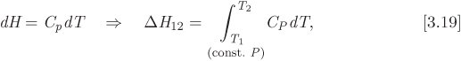
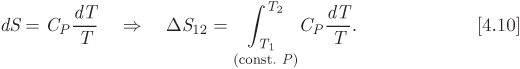
These results are not new, we encountered them previously in Chapters 3 and 4. That we recover them here serves a test of the validity of eqs. (5.24) and (5.26).
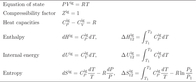
5.5 Ideal-Gas State
The calculation of enthalpy and entropy according to eqs. (5.24) and (5.26) requires the equation of state. Our first application will be in the ideal-gas state. Starting with the ideal-gas law, we compute the derivative (∂V/∂T)P:
For the coefficient of the dP term in the enthalpy equation we find:
Applying these results to eqs. (5.24) and (5.26):
These results are not new, they are the differential forms of eqs. (3.33) and (4.21), obtained previously. For the internal energy, we use the definition of enthalpy to write U = H − RT, and take its differential:
dUig = dHig − RdT,
and use eq. (5.27) for dHig:
Here we identify the multiplier of dT as the constant-volume heat capacity, that is,
Thus we have recovered all the results obtained previously by independent methods. The ideal-gas properties are summarized in Table 5-2.
Table 5-2: Summary of ideal-gas equations
5.6 Incompressible Phases
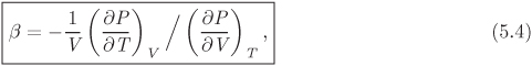
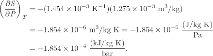
The effect of pressure on enthalpy and entropy is described by the dP term in eqs. (5.24) and (5.26). The partial derivative that appears in this term can be expressed in terms of the coefficient of thermal expansion as follows,
With this result, the equations for enthalpy and entropy become
For condensed phases (solids, liquids away from the critical point), both β and V are small. Accordingly, the contribution of the terms V (1−βT)dP and −βVdP to the enthalpy and entropy is generally negligible when compared to the contribution of the temperature term. This is the reason that we often take the enthalpy and entropy of compressed liquids to be independent of pressure. The accuracy of this approximation is tested in the example below.
V = V0 (1 + a1t + a2t2 + a3t3),
a1 = 1.3240 × 10⁻³, a2 = 3.8090 × 10⁻⁶, a3 = −0.87983 × 10⁻⁸.
V = 1.275 × 10⁻³ m3/kg.
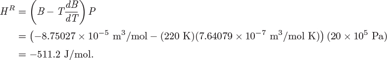
β = 1.454 × 10⁻³ K−1.

CP = 126.636 J/mol K = 2.180 kJ/kg K,
5.7 Residual Properties
The calculation of properties in the ideal-gas state, summarized in Table 5-2, is straightforward: the equation of state is simple to manipulate, and the heat capacity is independent of pressure, which further simplifies the calculation. This simplicity is lost when we move away from the ideal-gas state. The difficulty is not so much that the equation of state is now more complex, the computer will take care of that, but rather that the heat capacity becomes a function of both temperature and pressure. It would be possible, with some effort, to tabulate the heat capacity in terms of temperature and pressure. Fortunately, this is not necessary. The difficulty is removed through the introduction of residual properties. In this approach, the calculation is done in two parts: first we obtain enthalpy and entropy as if the substance were in the ideal state, then we add an appropriate correction that makes the result exact. This correction is the residual property. Given a property F(P, T), the corresponding residual property, FR(P, T) is defined by the equation,
where Fig is the ideal-gas property at pressure P and temperature T, namely, the property obtained by applying the ideal-gas equations. Residual properties can be defined for any thermodynamic property that can be expressed as a function of pressure and temperature, that is, for all properties except pressure and temperature themselves. For a change of state, eq. (5.31) gives:
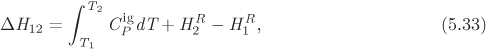
where ![]() is calculated by the ideal-gas equations, shown in Table 5-2. For enthalpy and entropy, specifically, eq. (5.32) takes the form,
is calculated by the ideal-gas equations, shown in Table 5-2. For enthalpy and entropy, specifically, eq. (5.32) takes the form,
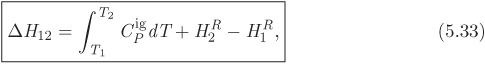
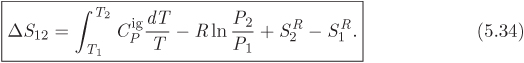
The usefulness of the residual properties should now be clear: the calculation of ΔH and ΔS reduces to the calculation of the residual enthalpy and entropy at the initial and final state. Notice that the only heat capacity that is needed in this calculation is the ideal-gas ![]() , which is available from tables. Of course, we still need expressions for these residuals. As it turns out, in deriving eqs. (5.24), (5.26), we have done most of the work already.
, which is available from tables. Of course, we still need expressions for these residuals. As it turns out, in deriving eqs. (5.24), (5.26), we have done most of the work already.
The Hypothetical Ideal-Gas State
In eqs. (5.33) and (5.34), the ideal-gas part represents a step of the calculation, a purely mathematical operation that computes the ideal-gas terms by the equations in Table 5-2. Sometimes we describe this part of the calculation by saying that the system is brought to the ideal-gas state at its own pressure P and temperature T. The “ideal-gas state at the system’s own pressure and temperature” exists only as a mathematical operation, not as a physical state. If we insist on ascribing physical meaning to it, we would describe it as state in which molecular interactions are turned off, so that molecules act as point masses at the pressure and temperature of the system; this system would act as an ideal gas, no matter how high the pressure, and regardless of whether the actual phase is a gas, liquid, or solid. Of course, in the physical world we cannot turn molecular interactions on and off at will. In the virtual world of mathematics, we can. We call this the “hypothetical ideal-gas state,” to indicate that we are not referring to the actual state of the system but to a mathematical recipe.
Residual Enthalpy
To obtain an equation for the residual enthalpy, we write HR = H − Hig and take its differential at constant temperature:
The term dH is given in eq. (5.24), the term dHig in eq. (5.27), and since temperature is constant, we set dT = 0 in both. This produces the following expression for the differential of the residual enthalpy:
Decreasing pressure to zero at constant T, we reach the ideal-gas state. At this limit the residual enthalpy vanishes because the enthalpy of system is exactly equal to the ideal-gas contribution. Thus, at P = 0, HR = 0, on all isotherms. We now integrate dHR from (P = 0, HR = 0), to (P, HR), along a line of constant temperature:
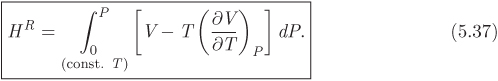
This is the desired result: it gives the residual enthalpy in state (P, T) in the form of an integral that may be evaluated if the equation of state is known.
Residual Entropy
An analogous equation for entropy is obtained in a similar manner. In analogy to eq. (5.35) we write
We use eqs. (5.26) and (5.28) for dS and dSig, respectively, and set dT = 0. Substituting these results to the above equation we obtain
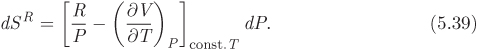
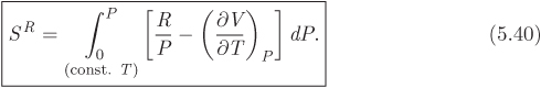
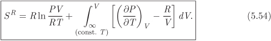
As with residual enthalpy, in the ideal-gas limit, SR = 0. Integration from P = 0, SR = 0 to P, SR, at constant temperature leads to the following result for the residual entropy:
Residual Volume
The residual volume is obtained by applying the definition of residual to volume. Using Vig = RT/P for the ideal-gas volume at pressure P and temperature T, the residual volume is
where V is the volume obtained from the equation of state. An alternative expression is obtained using the compressibility factor to write V = ZRT/P. Substituting this result into eq. (5.41) we obtain
which now gives the residual volume in terms of the compressibility factor.
Other Residual Properties
It is not necessary to derive equations for any other residual properties because these can all be related to VR, HR, and SR. In general, all relationships among “regular” properties can also be written among the corresponding residual properties. For example, internal energy is related to enthalpy through the relationship,
U = H − PV.
In the ideal-gas state, this becomes
Uig = Hig − PVig.
Taking the difference between the two, we obtain the relationship between the residual enthalpy and residual internal energy:
UR = HR − PVR.
We can now go ahead and write the similar equations for other properties. For example, for Gibbs free energy and Helmholtz free energy we have,
GR = HR − TSR,
AR = UR − TSR.
As we see, UR, GR, and AR can all be computed once HR, SR, and VR are known.
Applications
Equations (5.37) and (5.40) are suitable for calculations with equations of state. The general procedure is this: express the volume in terms of pressure and temperature, compute the partial derivative (∂V/∂T)P and finally perform the integrations in eqs. (5.37) and (5.40). The simplest possible equation of state is the ideal-gas law; in this case, the residuals should vanish. The next simplest case is the truncated virial equation. These are examined in the examples that follow. Cubic equations of state require some additional work and are discussed in Section 5.8.

Tc = 190.56 K, Pc = 45.99 bar.
5.8 Pressure-Explicit Relations
The importance of eqs. (5.37) and (5.40) is that they relate residual enthalpy and entropy to the equation of state. In the above form, these equations are useful if the equation of state can be expressed as function of pressure and temperature. Cubic equations express pressure in terms of volume and temperature; to calculate residual properties from such equations, eqs. (5.37) and (5.40) must be converted so that the independent variables are V and T. The mathematical manipulations are shown on next page.
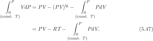
Enthalpy. We separate the integral in eq. (5.37) into two and work with each term separately:

To transform the first term, we start with the differential d(PV) = PdV + VdP, which we solve for VdP:
VdP = d(PV) − PdV.
Next, we integrate both sides from P = 0 to P along a line of constant temperature, T. Noting that the lower limit is the ideal-gas state, we have:
Now we work on the second integral in eq. (5.46). We start with the triple-product rule in eq. (5.3), and split the derivative (∂P/∂V)T to obtain
Using this result, the second integral in eq. (5.46) becomes
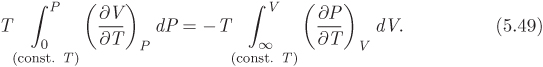
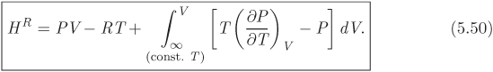
In all integrals, the lower limit is the ideal-gas state. When integration is with respect to pressure, the lower limit is P = 0; when it is with respect to volume, the lower limit is V = ∞. Substituting eqs. (5.47) and (5.49) into (5.46), we obtain the desired result:
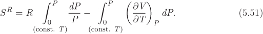
Entropy. A similar equation is obtained for entropy. We begin with eq. (5.40), which we write in the form,
We begin with the relationship P = ZRT/V and take the logarithm of both sides:
ln P = ln Z + ln R + ln T − ln V.
We now take the differential of both terms under constant temperature:
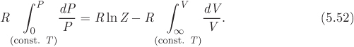
We integrate both sides under constant temperature from the ideal-gas (P = 0, V = ∞, Z = 1) state up to the current state (P, Z, V), and multiply both side by R, to obtain the following expression for the first integral in (5.51):
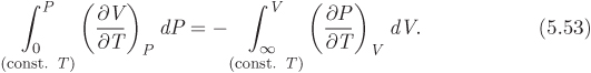
Using eq. (5.48) obtained above, the second integral is
Combining eqs. (5.52) and (5.53) into (5.51) we obtain the final result in the form
Both eqs. (5.50) and (5.54) are expressed as integrals in V. These integrals are evaluated along an isotherm, starting at the ideal-gas state and ending at the state of interest.
5.9 Application to Cubic Equations
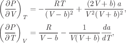
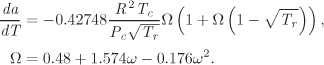
Equations (5.50) and (5.54) are now in suitable form for use with cubic equations of state. The general procedure is this: use the equation of state to calculate the partial derivative (∂P/∂T)V, then perform the integrations in eqs. (5.50) and (5.54). We demonstrate the procedure using the Soave-Redlich-Kwong equation. The pressure in the SRK equation is given by
Noting that the parameter a is a function of temperature, the partial derivative of pressure with respect to T is,
from which we obtain,
Inserting into eq. (5.50), the residual enthalpy is
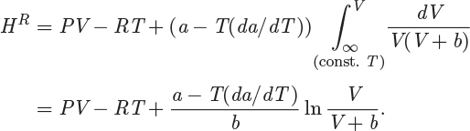
The result may be expressed in the alternative form,

where we have used V = ZRT/P to eliminate V in favor of Z, and B′ = Pb/RT is the dimensionless parameter previously defined in eq. (2.36). This streamlines the calculation of the residual enthalpy since working with the compressibility form of the equation of state is generally preferable. The residual entropy is obtained in the same manner, and the final result is

The derivative da/dT, which is needed for the calculation, is

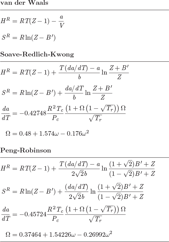
These results are summarized in Table 5-3, which also includes results for the van der Waals and the Peng-Robinson equation. In all cases, B′ is defined as B′ = Pb/RT, where b is the corresponding parameter in the equation of state.
The important conclusion is that residual properties can be calculated from the equation of state. The general procedure is this: at given T and P, first solve for Z, then apply the equations for the residual enthalpy and entropy. If the cubic equation for Z has three positive roots, the proper root must be selected based on the phase of the system. The calculation is demonstrated in the examples that follow.
Table 5-3: Residual properties from cubic equations of state
Tc = 282.35 K, Pc = 50.418 bar, ω = 0.0866.

Z3 − Z2 + 0.28682 Z − 0.0202872 = 0.
Z1 = 0.105351, Z2 = 0.360538, Z3 = 0.534111.


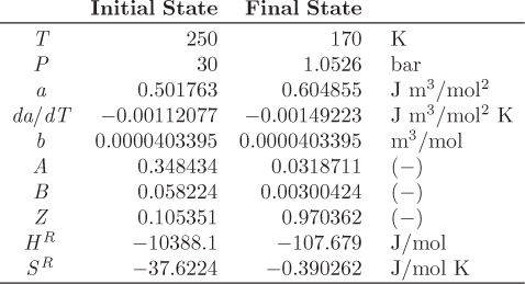
Enthalpy. The ideal-gas enthalpy is calculated by evaluating the integral of ![]() between the temperatures of the two states:
between the temperatures of the two states:
ΔH12 = (−2906.5) + (−107.679) − (−10388.1) = 7373.94 J/mol.
Entropy. The ideal-gas entropy change is
ΔS12 = (13.9014) + (−0.390262) − (−37.6224) = 51.1335 J/mol K.

5.10 Generalized Correlations
In the previous section we discussed the calculation of residual properties from cubic equations of state. The calculations are straightforward, though somewhat time consuming. A quicker alternative is to use generalized graphs. In Chapter 2 we discussed the Pitzer method for calculating the compressibility factor in terms of reduced temperature, reduced pressure, and acentric factor. Analogous equations can be obtained for the residual enthalpy and entropy. In this approach, the residual enthalpy, made dimensionless by the product RTc, is computed as
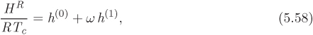
and the residual entropy, made dimensionless by R, is given by
Here, h(0), h(1), s(0), s(1), are dimensionless functions of the reduced temperature and reduced pressure, and common for all fluids. Lee and Kesler have computed these factors and the results are shown in Figures 5-2 and 5-3. These graphs may be used for quick estimations of the residual properties. The same cautionary comments made in Section 2.4 apply here as well, namely, that these charts may be used with normal fluids but not with fluids that are highly polar or strongly associating.
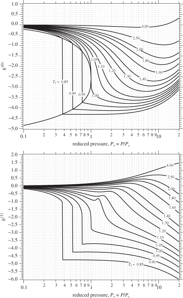
Figure 5-2: Lee-Kesler generalized graphs for the residual enthalpy.
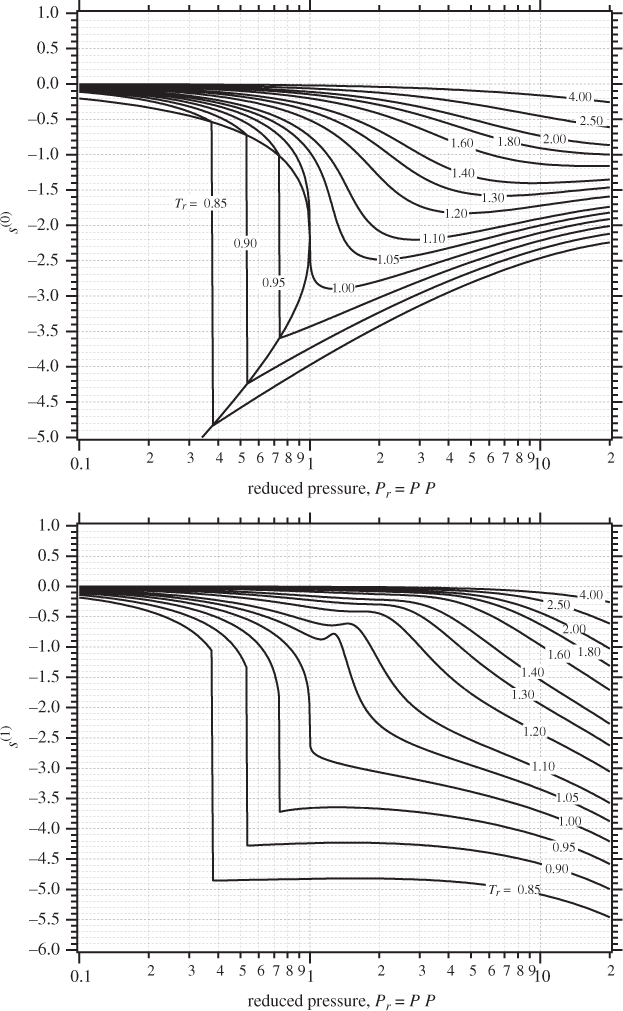
Figure 5-3: Lee-Kesler generalized graphs for the residual entropy.
Tc = 282.35 K, Pc = 50.418 bar, ω = 0.0866.
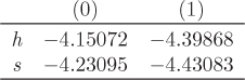
HR = (RTc)(−4.53164) = (8.314 J/mol K)(282.35 K)(−4.53164) = −10637.8 J/mol.
SR = − 4.61466R = (−4.61466)(8.314 J/mol K) = − 38.3663 J/mol K.
5.11 Reference States
The equations we have developed up to this point can be used to calculate differences in enthalpy and entropy between states. To calculate absolute values we must also know the actual value of enthalpy and entropy at some state. This actual value, however, is not important if our ultimate interest is in calculating differences. Indeed, in all problems of practical interest, this will be the case.6 And yet, it is convenient to calculate properties on absolute scale, as the steam tables demonstrate, because then differences can be calculated simply as algebraic differences between the values of a property at two states. Absolute properties are really differences from a state that we accept as a reference. This is common practice for many physical quantities, including potential energy, elevation, even kinetic energy.7 To the extent that the choice of the reference does not affect differences, reference states may be chosen arbitrarily. With respect to enthalpy and entropy, the choice is usually made so as to simplify the overall calculation.
6. In fact, both the first and the second law were formulated in terms of differences, rather than absolute values.
7. When we say that a car is traveling at a speed of 100 km per hour, we mean its speed with respect to the Earth, which itself is rotating around its own axis, moves around the sun, and travels with the solar system through the cosmos. These speeds are enormous. A car parked somewhere on the equator is actually rotating around the Earth’s axis at about 1700 km per hour. Yet, it does not get a speeding ticket because with respect to the road it is at rest.
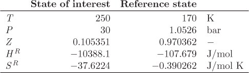
To develop an equation for the absolute properties, we start with eq. (5.31) and apply it to the enthalpy of the system at the state of interest, P, T, and at a reference state P0, T0, where the value H0 of the enthalpy is presumed known:
where the subscript 0 is for the reference state, and unsubscribed properties are at the state of interest. We take the difference and solve for H:
where ![]() is the ideal-gas enthalpy difference between the actual state and the reference state,
is the ideal-gas enthalpy difference between the actual state and the reference state,

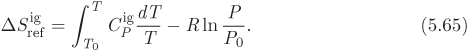
The corresponding equation for entropy is
with
To complete the calculation, we must specify the numerical values of all properties at the reference point, namely, H0, ![]() , S0, and
, S0, and ![]() . Two common conventions are the following:
. Two common conventions are the following:
• Actual enthalpy and entropy at (P0, T0) are set to zero. By this convention we set H0 = 0 and S0 = 0.8 The absolute enthalpy and absolute entropy are obtained from eqs. (5.62) and (5.64), which now become
8. The value of H0, S0, may be set to any constant, not necessarily zero. However, unless explicitly stated otherwise, we will take these constants to be zero.
This calculation requires the residual enthalpy and entropy at the refence state. These are constant and only need to be evaluated once. If the system at the reference pressure and temperature exists in multiple phases, the reference phase must be specified as well. For the steam tables, for example, the reference state is the saturated liquid at the triple point.
• Ideal-gas enthalpy and entropy at (P0, T0) are set to zero. By this convention we set the ideal-gas properties to zero: ![]() and
and ![]() . From eq. (5.61) then, we obtain
. From eq. (5.61) then, we obtain ![]() , and for the entropy,
, and for the entropy, ![]() . With these results in eqs. (5.62) and (5.64), the absolute enthalpy and absolute entropy become
. With these results in eqs. (5.62) and (5.64), the absolute enthalpy and absolute entropy become
In this convention, therefore, we fix properties of the hypothetical ideal-gas state and refer to it as the hypothetical ideal-gas reference state at the specified pressure and temperature.
Mathematically, the only difference between the two conventions is in the additive terms ![]() and
and ![]() . Both conventions, therefore, produce identical differences. The convention by which the actual properties at the reference state are set to zero is straightforward and makes physical sense: all enthalpies and entropies are measured relative to their values at the reference state. The hypothetical ideal-gas reference state is a bit simpler numerically, as it does not require the calculation of the residuals
. Both conventions, therefore, produce identical differences. The convention by which the actual properties at the reference state are set to zero is straightforward and makes physical sense: all enthalpies and entropies are measured relative to their values at the reference state. The hypothetical ideal-gas reference state is a bit simpler numerically, as it does not require the calculation of the residuals ![]() and
and ![]() , but is less straightforward to explain physically because it involves a hypothetical state. In either case, the reference state should be understood as a numerical recipe for the calculation of the absolute enthalpy and entropy.
, but is less straightforward to explain physically because it involves a hypothetical state. In either case, the reference state should be understood as a numerical recipe for the calculation of the absolute enthalpy and entropy.
The new results differ by ![]() for enthalpy, and
for enthalpy, and ![]() for entropy.
for entropy.
5.12 Thermodynamic Charts
A useful representation of the properties of pure fluids is in the form of graphs. Thermodynamic charts, although not convenient for large-scale calculations, such as those required in the design of chemical processes, are very useful in visualizing a processe and in obtaining the solution to small-scale problems graphically. A thermodynamic chart consists of two primary properties that are chosen as the axes and contains additional information in the form of phase boundaries and contours of various properties. The PV and ZP diagrams are examples of such charts that we encountered already. There is no limitation as to the properties that can be chosen to represent the axes and this freedom leads to various possible combinations. Three charts that find widespread use the pressure-enthalpy chart, the temperature-entropy chart, and the enthalpy-entropy chart, also known as Mollier chart. These are explained below.
Pressure-Enthalpy Chart
In this graph, shown in Figure 5-4, the vertical axis is pressure, usually in logarithmic scale, and the horizontal axis is enthalpy. The vapor-liquid boundary sits on the horizontal axis with the liquid region on the left and the vapor region on the right. The critical point is located at the very top of the vapor-liquid boundary. A horizontal line represents a constant-pressure process and a vertical line represents a constant-enthalpy (isenthalpic) process. Isotherms are lines with the general direction from the upper left to lower right corner. The shape of an isotherm depends on whether it is above or below the critical point. Starting from high pressure, a subcritical isotherm decreases sharply, intersects the phase boundary on the liquid side, moves horizontally to the saturated vapor, and resumes a sharp drop once in the superheated vapor region. The critical isotherm is tangent to the phase boundary at the critical point and bends noticeably in the region around it. Supercritical isotherms are shifted further up and do not intersect with the phase boundary. Isotherms are nearly vertical in the compressed liquid region (at high pressures to the left of the saturated liquid) and in the ideal-gas region (low pressures to the right of the saturated vapor). Both behaviors reflect the fact that enthalpy in the compressed liquid state and in the ideal-gas state is independent of pressure.

Figure 5-4: Pressure-enthalpy chart.
Temperature-Entropy Chart
In this chart temperature is plotted on the vertical axis and entropy on the horizontal axis, as shown in Figure 5-5. The vapor-liquid boundary sits on the horizontal axis with the liquid region to the left, vapor region to the right, and the critical point at the top. Isotherms on this graph are represented by horizontal lines. Isobars are lines of constant pressure and move in the general direction from the lower left corner to the upper right. Subcritical isobars intersect the saturated liquid, move horizontally until the saturated vapor, and move upwards once in the superheated vapor region. The critical isobar is tangent to the critical point, while supercritical isobars are shifted higher up and do not intersect the phase boundary. Isobars on the compressed liquid side are located very close to the saturated liquid, especially at temperatures below the critical. This is graphical manifestation of the fact that the entropy of the compressed liquid is very nearly equal to the entropy of the saturated liquid at the same temperature.
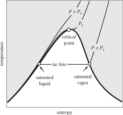
Figure 5-5: Temperature-entropy chart.
Enthalpy-Entropy Chart (Mollier Chart)
In this chart the vertical axis is enthalpy and the horizontal axis is entropy (Figure 5-6). This chart is commonly known as the Mollier diagram, after Richard Mollier, the German engineer and professor who pioneered the use of this chart for steam. The phase boundary sits on the horizontal axis but has some unusual features compared to the PH and TS graphs. The liquid region is to the left of the phase boundary and the vapor region to the right, but the critical point is not at the top of the curve but rather shifted towards the left. Tie lines are straight but not horizontal and generally move in a diagonal direction. A tie line is a line of constant temperature and constant pressure, that is, an isotherm inside the vapor-liquid region coincides with the isobar that corresponds to the saturation pressure at that temperature. Outside the vapor-liquid region the paths of the isotherm and the isobar separate: The isotherm turns to the right and becomes nearly horizontal, while the isobar (dashed line in Figure 5-6) continues to move upward. Isotherms and isobars also extend into the compressed liquid region (to the left of the saturated liquid) but these segments are not shown in Figure 5-6. The Mollier chart of steam is commonly used in calculations of steam turbines and compressors. Detailed Mollier charts found in the literature usually cover a smaller region than that shown in Figure 5-6 and focus mostly on the saturated line and the superheated vapor to the right of the critical point.

Figure 5-6: Enthalpy-entropy (Mollier) chart.
5.13 Summary
In this chapter we established various mathematical results, including relationships among various partial derivatives, and expressions for the differentials of properties with units of energy. The ultimate purpose of these derivations, and the most practical results of this chapter, are eqs. (5.33) and (5.34), which allow us to calculate enthalpy and entropy differences between any two states. This calculation requires two properties the ideal-gas heat capacity, and the equation of state. This is a result of great practical importance: it leads us to conclude that these two properties carry the entire thermodynamic DNA, so to speak, of any physical system.
The calculation of properties requires the residual enthalpy and entropy. These are intermediate properties and may be understood as corrections to the ideal-gas equations due to intermolecular interactions. If interactions could be turned off, the residual terms would drop off and all that is left then is the ideal-gas contribution. In contrast with the real ideal-gas state, which is reached by reducing pressure at constant temperature, this hypothetical ideal-gas state is reached, hypothetically of course, at constant temperature and pressure by turning off interactions.
To calculate the residual properties we have two options: using an equation of state, such as the Soave-Redlich-Kwong, or using the Pitzer correlation along with the Lee-Kesler charts. The latter method is also based on an equation of state (Benedict-Webb-Rubin), but the results are given in graphical form, thus eliminating the need for lengthy numerical calculations. The need for graphical solutions is largely obsolete today, as desktop and hand-held computers are capable of very sophisticated calculations at high speeds.
A final comment on reference states. This subject is often a source of confusion to students, but there is no reason why it should be this way. A reference state represents a point from where we choose to measure things. We measure altitudes from sea level, but we might as well measure them from downtown State College, PA. If we were to do that, all mountains would become about 1500 ft shorter, but they would all decrease by the same amount, so when we calculate the vertical rise between any two locations on Earth using the new reference state, we would still get the same answer. Ultimately, a reference state adds a constant number to whatever we measure. Because this constant drops out when we calculate differences, it doesn’t matter how we pick the reference point. We could measure altitudes from the center of the Earth and the fact that such choice sounds “unreasonable” does not mean we cannot use it.9 If we specify a state at P0, T0, to be the reference, we mean that all enthalpies and entropies are reported as differences from that state. When we specify the ideal-gas state at P0, T0, we mean to say enthalpy and entropy are to be calculated as differences from the corresponding H and S that the substance would have at P0, T0, if we used ideal-gas equations to calculate them. But it is easier to simply say that the ideal-gas reference state means, “use eqs. (5.68), (5.69) to calculate enthalpy and entropy.”
9. What is so reasonable about sea level? It is not even level!
5.14 Problems
Problem 5.1: a) Show that the variation of the CP with pressure at constant temperature is given by
b) Use this result to show that the CP and CV in the ideal-gas state are independent of pressure.
c) If the expansion coefficient β of a liquid is assumed to be approximately independent of pressure, what do you conclude for the relationship between CP and pressure in the compressed liquid state?
Problem 5.2: A gas is described by the state equation P(V − b) = RT where b is constant.
a) Obtain the residual entropy, enthalpy and internal energy as a function of pressure and temperature
b) Carbon dioxide undergoes reversible isothermal expansion in a turbine from PA = 20 bar to PB = 1 bar at a constant temperature of 300 K. Assuming that CO2 is described by the above state equation with b = 44.1 × 10⁻⁶ m3/mol, calculate ΔH, ΔS, the work produced and the amount of heat rejected or absorbed by the gas during the expansion.
Problem 5.3: Following a procedure analogous to that in Example 5.2, obtain an expression for the coefficient of thermal expansion based on the van der Waals equation of state. Use the result to calculate the value of β for oxygen at 20 °C, 30 bar.
Problem 5.4: Using the volume-temperature relationship for liquid acetone in Example 5.6 calculate the amount of heat and work involved when acetone is compressed isothermally and reversibly from 1 bar, 20 °C to 10 bar.
Problem 5.5: Estimate the constant-pressure heat capacity of oxygen at −50 °C, 38 bar, using the truncated virial equation. Hint: Use the truncated virial to calculate the enthalpy at two temperatures near −50 °C, 38 bar, then obtain the heat capacity by numerical differentiation.
Problem 5.6: Estimate the CP of liquid hexane at 1 bar, 20 °C using the SRK equation of state. For a hint, see problem 5.5.
Problem 5.7: Perry’s Handbook (Perry’s Chemical Engineers’ Handbook, 7th ed.) gives the ideal-gas heat capacity in the form,
(see Table 2-198, p. 2-178 in the 7th ed. of Perry’s Chemical Engineers’ Handbook).
a) Calculate the ideal-gas capacity of hydrogen cyanide at 300 K and report the value in J/mol K and in Btu/lbmol °F.
b) Calculate ![]() and
and ![]() in the temperature range 0 °C to 1000 °C (in J/mol K and in Btu/lbmol °F).
in the temperature range 0 °C to 1000 °C (in J/mol K and in Btu/lbmol °F).
c) Calculate ΔHig and ΔSig of HCN for a change of state from 1 bar, 0 °C to 15000 mmHg, 1000 °C. Report the results for enthalpy in J/mol and in Btu/lbmol; report entropy in J/mol K and Btu/lbmol °F.
Additional data: The following identities may be helpful:

Problem 5.8: a) What is the residual volume of saturated liquid water at 1 bar?
b) Estimate the residual volume of ethanol vapor at 1 bar and 100 °C.
c) Use the generalized graphs to calculate the entropy change of 1 mole of ethanol undergoing isothermal compression from 1 bar to 100 bar along the critical isotherm.
Problem 5.9: n-Octane is compressed reversibly at constant temperature along the critical isotherm until the critical point is reached. The initial pressure is 1 bar. The pressure takes place in a closed system. Use the Lee-Kesler method to calculate the following:
a) What is the entropy change of n-octane?
b) Calculate the heat that must be supplied to the system to maintain isothermal conditions.
c) Calculate the necessary amount of work.
Problem 5.10: Propane is isothermally compressed from 0.01 bar, −51.4 °C to 17 bar. The process takes place reversibly in a closed system.
a) Draw the PV graph of the process.
b) Calculate the entropy change of propane.
c) How much heat is exchanged between the system and its surroundings? Is this heat added to or removed from the system?
Additional data: Use the Lee-Kesler graphs for enthalpy and entropy. The saturation pressure of propane at −51.4 °C is 0.66 bar. Take the ideal-gas CP of propane at these conditions to be constant and equal to 67 J/mole K.
Problem 5.11: Isobutane is heated in a heat exchanger from 1 bar, 220 K to 300 K. Use the SRK equation to calculate the following:
b) The entropy generation if the heat is provided by a bath at 300 K.
Additional information: The ideal-gas heat capacity of isobutane is ![]() J/mol K.
J/mol K.
Problem 5.12: Oxygen is compressed by reversible adiabatic process in a closed system, from 1 bar, 20 °C to 10 bar. Assuming oxygen to follow the SRK equation of state, calculate the amount of required work. Hint: Tabulate the entropy of oxygen at 10 bar at various temperatures and locate the temperature where the entropy is equal to that at 1 bar, 20 °C.
Problem 5.13: Using as reference state the hypothetical ideal-gas state at 70 K, 7.83 bar, and with the data given below, calculate the following.
a) The enthalpy of nitrogen at 70 K, 7.83 bar.
b) The enthalpy of saturated liquid nitrogen at 7.83 bar.
c) The enthalpy of vaporization of nitrogen at 7.83 bar.
Additional data:

Problem 5.14: Use the SRK equation to calculate the following properties of isobutane:
a) Residual enthalpy and entropy at 10 bar, 300 K.
b) Enthalpy and entropy at 10 bar, 300 K using as reference state the saturated liquid at 1 bar (Tsat = 266 K).
c) Enthalpy and entropy at 10 bar, 300 K using as reference state the hypothetical ideal-gas state at 1 bar 266 K.
d) Enthalpy and entropy of vaporization at 1 bar.
The ideal-gas constant-pressure heat capacity may be taken to be constant and equal to 96.5 J/mol K.
Problem 5.15: Calculate the enthalpy and entropy of isobutane at 1 bar, 300 K, and 1 bar, 250 K using as reference state:
a) The actual state at P = 20 bar, T = 400 K.
b) The ideal-gas state at P = 20 bar, T = 400 K.
In each case calculate the amount of heat for constant pressure cooling of isobutane from 1 bar, 300 K to 250 K, and the entropy generation if cooling takes place inside a bath at Tbath = 240 K. The following data are available:

Problem 5.16: Use the Lee-Kesler method to do the following:
a) Calculate the entropy of propane at its critical point. The reference state is the ideal-gas state at the critical point.
b) Calculate ΔS of propane for an isothermal process that takes the substance from its critical point to pressure 1 Pa.
c) A member of our engineering team objects that the reference state is not valid because a substance is not ideal at the critical point. What is your response?
Problem 5.17: The steam tables are calculated with reference state the saturated liquid at the triple point (Ptriple = 0.006117 bar, Ttriple = 0.01 °C). Suppose we want to retabulate the properties of steam using a different reference state. Show how this can be done by calculating V, U, H, and S at 1 bar, 200 °C using the following reference states:
a) the saturated vapor at 10 bar;
b) the saturated vapor in the hypothetical ideal-gas state at 10 bar.
Additional data: The ideal-gas heat capacity of water is given by the following equation with T in kelvin.