Chapter 10. Theory of Vapor-Liquid Equilibrium
When a fluid is brought into the vapor-liquid region, it forms two coexisting phases, each with its own molar properties (volume, enthalpy, entropy, etc.). If the fluid is a mixture of components, then each phase also has its own composition. This fundamental property of mixtures is the basis of separation processes. A major goal of chemical engineering thermodynamics is to provide computational methodologies for the calculation of phase diagrams in systems with many components. This requires the determination of the precise conditions that lead to phase separation, the number of phases that form, and their composition. The thermodynamic property that holds the answers to these problems is the Gibbs free energy.
In this chapter we will learn how to:
• Develop the fundamental equations of phase equilibrium in terms of the chemical potential and fugacity.
• Calculate fugacity from an equation of state.
• Calculate vapor-liquid equilibrium of a mixture using the equation of state.
10.1 Gibbs Free Energy of Mixture
In Chapter 4 we determined that the equilibrium state of a closed system at constant temperature and pressure corresponds to conditions that minimize the Gibbs free energy:
For a mixture that contains ni moles of component i with i = 1, 2, ... N, this inequality remains valid provided that the moles of all components are held constant:1
1. In our notational convention, subscript ni indicates that all ni, with i = 1, 2, ..., N, are held constant.
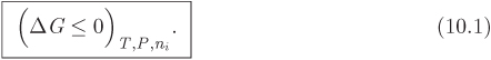
the equilibrium state of a multicomponent system whose temperature, pressure, and number of moles of all components are fixed, is a state that minimizes the Gibbs free energy.
This is a statement of fundamental importance in thermodynamics and the starting point for the discussion of phase equilibrium. To apply it we must first develop expressions for the Gibbs free energy of multicomponent systems. We begin by writing the differential of G in the standard form,

The derivatives with respect to temperature and pressure were obtained previously in Chapter 5:
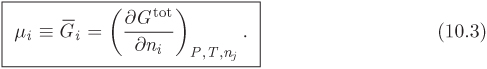
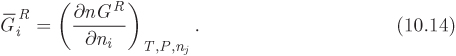
These were originally derived for a pure component, but they apply to all systems of constant composition, of which the pure component is a special case.2 The partial derivatives with respect to ni on the right-hand side of eq. (10.2) are the partial molar Gibbs free energies (![]() ) with respect to each component. The partial molar Gibbs free energy is a very important property. For this reason it is given a special name, chemical potential, and a special symbol, μi:
) with respect to each component. The partial molar Gibbs free energy is a very important property. For this reason it is given a special name, chemical potential, and a special symbol, μi:
2. See also relevant discussion in Chapter 9.
Using this definition and eqs. (5.18), the differential of the Gibbs free energy of mixture is written in the more compact form,

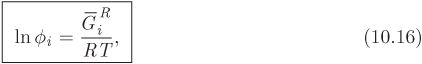
This is the fundamental equation for the Gibbs free energy of mixture in terms of temperature, pressure, and number of moles of all components. An alternative form of this equation, which will be useful in subsequent developments, is obtained by developing an expression for the differential of the ratio Gtot/RT, which is dimensionless. We start by calculating the differential of this ratio:
For dGtot we substitute eq. (10.4), for Gtot we substitute Htot − TStot, and with some straightforward manipulation the result is

This expression is equivalent to eq. (10.4). It has the advantage that it is in dimensionless form and involves the enthalpy, rather than the entropy of the mixture.
Multicomponent Equilibrium
When a mixture is brought into the two-phase region, it splits into two phases, each with its own composition. The situations is shown schematically in Figure 10-1. On a microscopic basis, molecules of both components pass continuously from one phase to the other. It is this molecular transfer that allows the system to find and maintain its equilibrium composition. When this composition is reached, the net transfer between phases is zero. Molecules continue to cross the interface in such way that the rate of transfer in one direction matches the rate in the reverse direction, so that the average (macroscopic) composition of each phase remains constant. We analyze this situation as follows. We form a mixture by mixing n1 moles of component 1 with n2 mols of component 2, and fix the temperature and pressure of the system. Next, we take an arbitrary number ![]() moles of component 1 and
moles of component 1 and ![]() moles of component 2 and place them in the vapor phase, with the remaining moles placed in the liquid. Out of the infinitely many ways that the two components can be partitioned between the two phases, only one corresponds to the true equilibrium state. To identify the equilibrium state we apply the Gibbs inequality in eq. (10.1): since the Gibbs free energy must be at a minimum, if we transfer a small amount δni of component i from one phase to the other, the Gibbs energy must remain unchanged. That’s because this change takes place at the bottom of the Gibbs curve (see Figure 4-7) where its derivative is flat. Suppose that we transfer δni mole of component i from the liquid to the vapor. The change in the Gibbs energy of the liquid is −
moles of component 2 and place them in the vapor phase, with the remaining moles placed in the liquid. Out of the infinitely many ways that the two components can be partitioned between the two phases, only one corresponds to the true equilibrium state. To identify the equilibrium state we apply the Gibbs inequality in eq. (10.1): since the Gibbs free energy must be at a minimum, if we transfer a small amount δni of component i from one phase to the other, the Gibbs energy must remain unchanged. That’s because this change takes place at the bottom of the Gibbs curve (see Figure 4-7) where its derivative is flat. Suppose that we transfer δni mole of component i from the liquid to the vapor. The change in the Gibbs energy of the liquid is −![]() while the change in the vapor is
while the change in the vapor is ![]() . For the total Gibbs energy to remain constant, we must then have
. For the total Gibbs energy to remain constant, we must then have
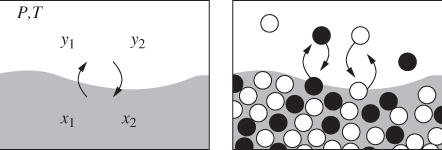
Figure 10-1: Macroscopic and molecular view of vapor-liquid equilibrium.
This expresses a very important result: in equilibrium between phases, the chemical potential of each component is the same in both phases.
Gibbs’s Phase Rule
Equation (10.6) is a general criterion that applies not just to vapor-liquid systems, but to systems with any number of phases. As an example, at the triple point of a pure substance where liquid, vapor, and solid coexist, the chemical potential is the same in all three phases:
μS = μL = μV.
A pure substance can simultaneously exist in three phases at most. With mixtures it is possible to observe coexistence of more phases. For example, two partially miscible liquids form two separate liquid phases. At its boiling point, such system consists of three phases, two liquids plus vapor; if a solid is added at amounts that exceed its solubility limit in both phases, the undissolved solid constitutes an additional phase. In general, by increasing the number of components we gain more degrees of freedom and it is possible to form more coexisting phases. A systematic way to count the degrees of freedom is provided by Gibbs’s phase rule.
We consider a system with N components distributed among π phases. To specify the intensive properties of this system we need to know pressure, temperature, and the mol fractions in each phase. There are N − 1 mole fractions in each phase,3 or (N − 1) π in total. Along with pressure and temperature, the total number of unknowns is
3. The Nth mole fraction is obtained from the normalization condition, x1 + x2 + ... = 1.
2 + π(N − 1).
The equations that are available to solve for these unknowns are given by the equilibrium condition: for each component i, the equilibrium criterion demands equality of the chemical potentials in each phase. Thus we have the following equations
This gives π − 1 equations4 for each component, or N(π − 1) equations in total. The number of degrees of freedom is the difference between the unknowns and the equations available:
4. In a series of equalities of the form a = b = ... = z, in which each term appears only once, the number of independent equations is equal to the number of equal signs.
F = 2 + π(N − 1) − N(π − 1),
This equation is known as Gibbs’s phase rule. One application of the phase rule is to determine the number of variables that must be specified to fully define the state of the system. For a single-phase pure component (N = 1, π = 1) the phase rule gives F = 2, namely, that to fix the state we must specify two variables (pressure and temperature, or some other combination). Increasing the number of phases decreases the degrees of freedom. For a two-phase pure substance, only one variable is needed; indeed at saturation we may specify the pressure of the system or its temperature, but not both, since knowing one fixes the other. Another application of the phase rule is to determine the maximum number of phases that are possible. This corresponds to setting the degrees of freedom to zero (the degrees of freedom cannot be negative). For a single component we find πmax = 3 while a binary mixture, πmax = 4.
10.2 Chemical Potential
The chemical potential is an important property in phase equilibrium, its importance arising from the equilibrium criterion, eq. (10.6). As a partial molar property, it satisfies eqs. (9.10) and (9.11), which now become
and
The chemical potential represents the molar contribution of a component to the Gibbs energy of the mixture. For a pure component (xi = 1, xj≠i = 0), the chemical potential is equal to the molar Gibbs energy
To make equations more readable we will use the symbol Gi to indicate the chemical potential of pure component, and μi for the chemical potential of component in a mixture.
Note
Gibbs-Duhem equation revisited
As a partial molar property, the chemical potential obeys the Gibbs-Duhem equation. This equation was derived in Chapter 9 (see eq. 9.12). Applied to the chemical potential it gives
In a two component mixture this becomes (see eq. 9.13)
This equation says that the chemical potential of components in a mixture do not change independently of each other with changing composition.
Chemical Potential in Ideal Gas and in Real Mixture
In Chapter 9 we obtained the following equation for the Gibbs free energy of a mixture in the ideal-gas state:
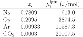
Comparing this with eq. (10.8), we identify the chemical potential ![]() , of component i in the ideal-gas mixture as
, of component i in the ideal-gas mixture as
where ![]() is the Gibbs free energy (chemical potential) of the pure component in the ideal-gas state.
is the Gibbs free energy (chemical potential) of the pure component in the ideal-gas state.
To obtain the chemical potential of component in a real mixture, we write the Gibbs free energy in terms of the residual Gibbs energy:
G = Gigm + GR,
and write the corresponding relationship among the partial molar properties of each term:
where ![]() is the partial molar residual Gibbs energy,
is the partial molar residual Gibbs energy,
Thus the calculation of the chemical potential is reduced into a calculation of the residual partial molar Gibbs energy.
where ![]() is the molar Gibbs energy of pure component at 1 bar, 25 °C. The reference state for each pure component specifies Hi = 0 and Si = 0. from this we obtain, Gi = Hi − TSi = 0. The chemical potential then simplifies to
is the molar Gibbs energy of pure component at 1 bar, 25 °C. The reference state for each pure component specifies Hi = 0 and Si = 0. from this we obtain, Gi = Hi − TSi = 0. The chemical potential then simplifies to
μi = RTln xi.
Gpure comp. − Gair = (0) − (− 1404.56) = 1404.56 J/mol.
Upon taking the difference, the ![]() terms cancel and the result is the familiar Gibbs energy of mixing.
terms cancel and the result is the familiar Gibbs energy of mixing.
10.3 Fugacity in a Mixture
In Chapter 7 we introduced fugacity and the fugacity coefficient as auxiliary variables related to the Gibbs energy of pure component. Here we extend these definitions to mixtures. The fugacity of component in mixture, fi, is defined as
where xi is the mole fraction of component in the mixture, P is pressure, and ϕi is the fugacity coefficient of component, defined as
where ![]() is the residual partial molar Gibbs energy. These definitions revert to those of the pure component by setting xi = 1, as one can easily verify. The ideal-gas limit of these properties is obtained by noting that the residual partial molar Gibbs energy in the ideal-gas state is zero:
is the residual partial molar Gibbs energy. These definitions revert to those of the pure component by setting xi = 1, as one can easily verify. The ideal-gas limit of these properties is obtained by noting that the residual partial molar Gibbs energy in the ideal-gas state is zero:
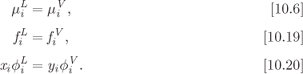
The fugacity of component in mixture is closely related to the chemical potential. Given two states of a mixture at the same temperature (but not necessarily at the same pressure or composition), the relationship between the chemical potentials and the fugacities in the two states is (see Example 10.3 for the derivation)
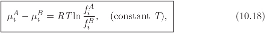
where A and B refer to two states of component i at the same temperature (the derivation is given as an example below). This is an important equation that establishes the relationship between the two properties and shows that fugacity is nothing but a mathematical transformation of the chemical potential. An important consequence of this result is obtained by applying eq. (10.18) to vapor-liquid equilibrium. Taking one state to be the liquid and the other the vapor, both states are at the same temperature, same pressure, but different composition. Since the chemical potential of a component is the same in both phases, eq. (10.18) states that the same is true for the fugacity:
Therefore, the criterion for phase equilibrium may be expressed either in terms of chemical potentials, or in terms of fugacity. Both approaches are equivalent and all problems in phase equilibrium may be solved using either one. We prefer to work with fugacity because its calculation does not require a reference state and because of its straightforward ideal-gas limit. Using eq. (10.15) to express fugacity in terms of the fugacity coefficient, and noting that pressure is the same in both phases, the equilibrium criterion becomes
where xi and yi are the mole fractions of component i in the liquid and the vapor respectively, and ![]() , are its fugacity coefficients in the two phases. In the special case of pure component (xi = yi = 1), the fugacity coefficients in each phase are equal. In the general case, the fugacity coefficients are not equal but satisfy eq. (10.20).
, are its fugacity coefficients in the two phases. In the special case of pure component (xi = yi = 1), the fugacity coefficients in each phase are equal. In the general case, the fugacity coefficients are not equal but satisfy eq. (10.20).
Solution We start with eq. (10.13) and use eq. (10.12) for ![]()
The term ![]() is the change of the ideal-gas Gibbs free energy of pure component between two pressures on the same isotherm. This is given by
is the change of the ideal-gas Gibbs free energy of pure component between two pressures on the same isotherm. This is given by
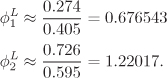
Solution The starting point is the equilibrium criterion in eq. (10.20), which relates the fugacity coefficients of a component to the mole fraction of the component in each phase. However, one coefficient must be known for the other to be calculated from this equation. In the absence of additional information, we must make some suitable approximations. We will assume that the vapor phase is ideal and take ![]() for both components. Then, the fugacity coefficient in the liquid phase is
for both components. Then, the fugacity coefficient in the liquid phase is

10.4 Fugacity from Equations of State
In Chapter 9 we discussed the use of equations of state for mixtures. Given the equation of state we may calculate all the residual properties of the mixture, including the residual Gibbs free energy. Since the fugacity coefficient is defined in terms of the residual partial molar Gibbs free energy, the equation of state may be used to calculate fugacity coefficients in gas and liquid mixtures. The calculation requires the application of the partial molar derivative to the residual Gibbs energy. Applying this mathematical operation to the composition-dependent terms of the residual Gibbs energy, we ultimately obtain an equation for the fugacity coefficient of the component. The equations below summarize the results for the two commonly used cubic equations of state:
• Soave-Redlich-Kwong

• Peng-Robinson

In both equations the dimensionless parameter Cʹi is defined as
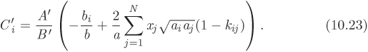
In writing these equations we follow the convention that parameters of the cubic equation with a single subscript (ai, bi) refer to pure components while unsubscribed parameters (a, b, Aʹ, Bʹ) refer to the mixture. Parameter Cʹi is introduced for convenience and combines parameters of the pure component and of the mixture. In the case of binary mixture, this parameter simplifies to:

The numerical steps for the calculation of the fugacity coefficient are analogous to those for the residual properties of mixture:
1. The required input is temperature, pressure, composition, and phase of the system (in case the compressibility equation has three real roots).
2. Calculate the parameters ai, bi, of the pure components.
3. Calculate the parameters a, b, of the mixture using the mixing rules from eqs. (9.38) and (9.39).
4. Calculate the parameters Aʹ and Bʹ of the mixture using eq. (2.36), and the parameter Ci for each component from eq. (10.23).
5. Solve for the roots of the compressibility factor: if there are three real roots, choose based on the phase of the system.
6. Calculate the fugacity coefficients from eqs. (10.21) or (10.22) using the compressibility factor of the mixture.
7. Calculate the fugacity of each component from eq. (10.15).
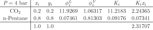
This calculation is demonstrated with a numerical example below.

Aʹ = 0.0525105, Bʹ = 0.0544159.
Z3 − Z2 + 0.467728Z − 0.028574 = 0,
Z = 0.0711422.
ϕ1 = 2.80821, ϕ2 = 0.02029.
f1 = (0.32)(2.80821)(16.15) = 14.5 bar,
f2 = (0.68)(0.02029)(16.15) = 0.223 bar.
10.5 VLE of Mixture Using Equations of State
We now have all the necessary ingredients to compute the phase diagram of a mixture based entirely on an equation of state. The starting point is the equilibrium condition, which for a binary system gives
The variables that define a tie line are pressure, temperature, and the mole fractions in the two phases. This makes for a total of four unknowns (only one mole fraction is needed per phase as the other is calculated from the normalization condition). Given four variables and two equations, two variables must be specified in order to solve for the rest.5 Depending on which variables are specified and which are unknown, VLE problems are classified according to the following scheme:
5. We obtain the same result by the phase rule: with two components (N = 2) and two phases (π = 2), the number of degrees of freedom is N +2 −π = 2.
• Bubble P. Temperature and liquid-phase composition are specified; solve for bubble pressure and vapor mol fractions.
• Bubble T. Pressure and liquid-phase composition are specified; solve for bubble temperature and vapor mol fractions.
• Dew P. Temperature and vapor-phase composition are specified; solve for dew pressure and liquid mol fractions.
• Dew T. Pressure and vapor-phase composition are specified; solve for dew temperature and liquid mol fractions.
• Flash. Pressure and temperature are specified; solve for the compositions of the two phases.
The bubble and dew problems are named according to the unknowns, for example, in the bubble P problem we are solving for bubble pressure and composition of the vapor in equilibrium with a known liquid. The flash problem is analogous to a flash separator in which pressure and temperature are fixed. To solve any of these problems all that is needed is an equation for the fugacity coefficient of the form,
ϕi = ϕi (P, T, compositions, phase),
such as eqs. (10.21) and (10.22). In computer language, the above expression represents a procedure that returns the fugacity of component i given temperature, pressure, composition, and phase (liquid or vapor). The phase must be indicated because it is needed for the selection of the proper root for the compressibility factor.
For a binary system, all of the above problems reduce to two equations that must be solved for two unknowns. However, the nonlinear character of the equations and the discontinuous character of the isotherms require a trial-and-error methodology. We outline below an iterative method for the solution of the bubble P problem. The calculation is streamlined by introducing the K -factors defined in Chapter 8,

The first equality is the definition of Ki, given in eq. (8.4); the second equality follows from the definition of fugacity, eq. (10.15). Using the K factors, the mole fractions in the vapor are
and obey the normalization condition
Equations (10.27) and (10.28) are solved iteratively as follows:
1. Start with a guess for the bubble pressure and the gas-phase mole fractions.
2. Calculate the fugacity coefficients of the liquid.
3. Calculate the fugacity coefficients of the vapor and the K factors of each component.
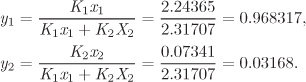
4. Obtain a refined estimate of the mole fractions using eq. (10.27):
Here, division by K1x1 + K2x2 is needed because the mole fractions calculated directly from eq. (10.27) will not obey the normalization condition except at the bubble pressure.
5. Check the value of K1x1 + K2x2: if it has changed from the previous iteration, return to step 3 and repeat the calculation with the new vapor mole fractions until this quantity does not change any more.
6. If the converged value of K1x1 + K2x2 is 1, we have obtained the solution; if not, refine the estimate for the pressure, return to step 2 and repeat. To obtain a new guess for the pressure, use the quantity K1x1 + K2x2 as a guide: if this quantity is larger than one, pressure is too high and should be decreased; if less than one, pressure is too low and should be increased. One way to adjust pressure systematically is to calculate the new guess using the equation below:
Such numerical details may be varied according to the system to improve the speed of convergence.
The calculation described here consists of two nested loops, an inner loop that refines the mole fractions of the vapor, and an outer loop that refines the estimate for pressure. Care must be exercised to identify trivial solutions. A trivial solution is one for which the liquid and vapor phases have the same composition and same compressibility factor. In this case the fugacity coefficients of a component are the same in the two phases (i.e., Ki = 1 for all components) and all equations are satisfied. Such solution is physically acceptable only at the critical point, but spurious solutions of this type may appear at other pressures and temperatures.
By this calculation we obtain one tie line on the phase diagram, defined by the values of pressure, temperature, and composition of the two phases:
{T, P, x1, y1}.
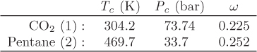
This tie line may be plotted on a Pxy or Txy graph. The entire phase diagram can be constructed in this manner by repeating the calculation at different conditions. Figure 10-2 shows the Pxy graph of the system carbon dioxide/n-pentane calculated by the Soave-Redlich-Kwong equation of state (see Example 10.6 for additional details of this calculation). The calculated phase diagram is in very good agreement with experimental data for this system. At 277.65 K, both components are below their critical temperature and the Pxy graph extends over the entire range of compositions. At 344.32 K, carbon dioxide is above its critical temperature (304.2 K) and the phase envelop is detached from the axis that represents pure CO2. The SRK calculation is very good in this case as well (close to the critical point of the mixture the numerical calculation converges very slowly and these points are not shown).
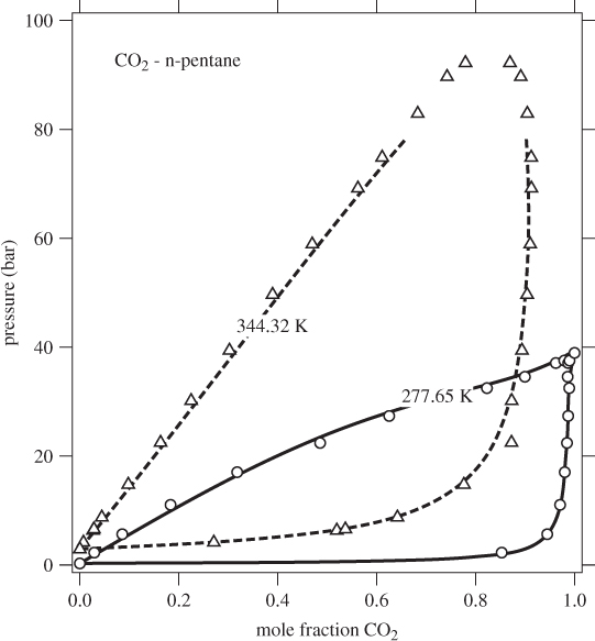
Figure 10-2: Pxy graph of carbon dioxide-n pentane calculated using the SRK equation with k12 = 0.12.
The Interaction Parameter
The interaction parameter is a required input for this calculation. It is an empirical parameter that must be obtained by fitting the calculated values from the equation of state to experimental data. For the calculations shown in Figure 10-2 the same value of interaction parameter was used in both temperatures. It is possible to obtain a better fit by allowing the interaction parameter to vary with temperature. For many systems, however, the interaction parameter is taken to be independent of temperature. A listing of k12 values for some binary systems is given in Sandler (Ref. [3]) for use with the Peng-Robinson equation. Though these values are specific to the Peng-Robinson equation, they may be used as a starting guess in the Soave-Redlich-Kwong equation. In general, before a serious calculation is undertaken based on an equation of state, the interaction parameter should be validated by comparison to data as extensively as possible.

Note
On Equations of State
The appeal of equations of state is that they can be used to obtain the entire phase behavior of a system over a wide range of pressures and temperature using tabulated values (critical properties, acentric factor) and a one adjustable parameter (interaction parameter). There are, however, two important limitations. The first one is that equations of state are generally applicable to small molecules that are chemically similar and interact via weak, nonpolar forces. While this encompasses many hydrocarbon systems that are industrially important, it excludes a much wider class of mixtures of strongly interacting molecules, including systems that contain water and other polar molecules. The second limitation is that these calculations quickly become cumbersome as the number of components increases. For this reason, alternative methods have been developed that can handle a broader variety of systems. The most widely used methodology is based on the notion of the ideal solution and makes use of activity coefficients. These topics are discussed in Chapters 11 and 12.
10.6 Summary
In this chapter we developed the criteria for phase equilibrium in a multicomponent mixture and showed how to construct the entire phase diagram if the equation of state is known. The most important theoretical result is equilibrium criterion which we expressed in the following equivalent forms:
The fundamental result is eq. (10.6), which equates the chemical potentials of a component in every phase the component is present. Equations (10.19)–(10.20) express the equilibrium criterion in terms of fugacity (or fugacity coefficient) and represent equivalent forms of eq. (10.6). Another important result is a relationship between chemical potential and fugacity:
This equation relates the chemical potential and fugacity at two states at the same temperature. This relationship allows us to use fugacity interchangeably with chemical potential to solve problems in phase equilibrium.
In general, calculations of phase equilibrium are reduced to calculations of fugacity and since fugacity can be calculated from an equation of state, the vapor-liquid problem of mixture can be solved if such equation is available. The required inputs are (1) an appropriate equation of state, (2) suitable mixing rules, and (3) the ideal-heat capacities of the pure components. The appeal of equations of state is that they require little more than tabulated values (critical properties, acentric factor) of the pure components. This convenience comes with a price: the method is not guaranteed to work for arbitrary mixtures. Generally, it works very well for similar compounds that are weakly interacting, usually mixtures of short hydrocarbon chains and other non-polar molecules, but fails with many other systems, including many aqueous solutions. This problem requires the development of alternative methodologies that do not suffer from this weakness. These are discussed in Chapters 11 and 12.
10.7 Problems
Problem 10.1: a) How many degrees of freedom are there at the triple point of a pure substance?
b) What is the fugacity of ice at the triple point? The triple point of pure water is at 0.611 kPa and T = 0.01 °C.
c) Calculate the Gibbs energy of ice at the triple point.
d) Calculate the fugacity and the fugacity coefficient of liquid water at 0.01 °C and 300 bar.
Problem 10.2: a) First define the fugacity coefficient, ϕ, of the mixture as
where GR is the residual Gibbs energy of the entire mixture. Then show that the fugacity coefficient of a species, ϕi, is related to the fugacity coefficient of the mixture as follows:
In other words, the logarithm of the fugacity coefficient—rather than the coefficient itself—is a partial molar property.
b) Based on your previous result, outline the procedure for the calculation of the fugacity coefficient of a component in a mixture using an equation of state such as the SRK.
Problem 10.3: At 50 °C, 1.2 bar, the system n-pentane (1), n-hexane (2), and n-heptane (3) exists in vapor-liquid equilibrium. The mole fractions in the two phases are: x1 = 0.6, x2 = 0.2, x3 = 0.2 in the liquid; and y1 = 0.87, y2 = 0.1, y3 = 0.03 in the vapor.
a) Calculate the fugacity and the fugacity coefficient of each component in the vapor and in the liquid.
b) Calculate the chemical potential of n-heptane in the liquid. The reference state is the ideal-gas state at 200 K, 35 bar.
Additional information: Ideal-gas heat capacity of n-heptane: CP = 200 J/mole K.
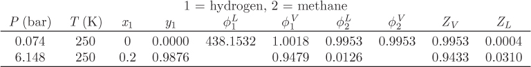
Problem 10.4: Your company faxed you some results, shown below, for the system hydrogen (1) / methane (2). Use these data to answer the following:
a) Because the fax machine malfunctioned, some entries were missing. Supply the missing numbers and explain your calculations.
b) What is the saturation pressure of methane at 250 K?
c) Calculate the fugacity of saturated liquid methane at 250 K.
d) Calculate the fugacity of methane at 250 K, 300 bar.
e) A solution with composition x1 = 0.2 is to be stored at 250 K. It is important to avoid the formation of vapor. What is the minimum pressure required?
f) Calculate the volume of the tank needed to store a saturated liquid mixture of the two components with composition x1 = 0.2 at 250 K. Report the result in cubic meters per million of mol.
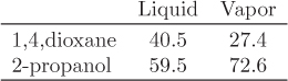
Problem 10.5: Calculate the ideal work for the separation of the following mixtures into their pure components. In all cases initial mixture as well as the purified components are at 10 °C, 1 bar. You may take the surroundings to be at 25 °C.
a) Gas mixture containing 25% Ne (1) + 75% H2 (2).
b) Gas mixture containing 25% methane (1) + 75% ethane (2).
c) Solution containing 25% ethanol (1) + 75% water (2). Additional data for this system at 10 °C, 1 bar are given below:

d) Compare the answers and suggest reasons why some of these results are the same and some are not.
Problem 10.6: At 89.8 °C, 0.75 bar, water (1) and pyridine form a vapor-liquid mixture with mol fractions x1 = 0.3114, y1 = 0.5411.
a) Calculate the fugacity of component in the vapor.
b) Calculate the fugacity coefficient of the two components in the liquid.
c) Calculate the molar Gibbs energy of the vapor and of the liquid. The reference state for each component is the ideal-gas state at 89.8 °C, 0.75 bar.
You may assume the gas phase to be in the ideal-gas state.
Problem 10.7: A box is divided into two compartments via a partition. Part A contains a mixture of nitrogen and oxygen in molar ratio N2 : O2 = 2 : 1. The second compartment is three times as big in volume as compartment A and contains pure oxygen. Both compartments are at 1 bar, 300 K, and the entire box is insulated from the surroundings. The partition is removed and the system is allowed to reach equilibrium.
a) Calculate the chemical potential of each component before and after the removal of the partition. As reference state, use the pure components at 1 bar, 300 K.
b) Calculate the fugacity of each component before and after the removal of the partition.
You may assume the components and their mixtures to be in the ideal-gas state at the pressures and temperatures of this problem. Is this a reasonable assumption?
Problem 10.8: The following table is a set of VLE data for methanol(1)/water(2) at 333.15 K.

a) What is the saturation pressure of methanol at 333.15 K?
b) What is the phase of the mixture that contains 50% (by mole) methanol at 333.15 K and 40 kPa?
c) At z1 = 0.2 and 30 kPa, the system is present as two phases. What is the chemical potential of methanol and water in the vapor phase using an ideal gas reference state at 300 K and 101 kPa? Is the assumption of treating the vapor phase as an ideal gas appropriate?
Additional information: The CP’s of methanol and water vapor are 49.0 and 33.8 J/mol K, respectively.
Problem 10.9: Use the SRK equation with k12 = 0 to compute the phase diagram of the system normal hexane (1)/normal octane (2) at the following conditions:
a) Pxy graph at 350 K.
b) Txy graph at 1 bar.
Make graphs and annotate them properly.
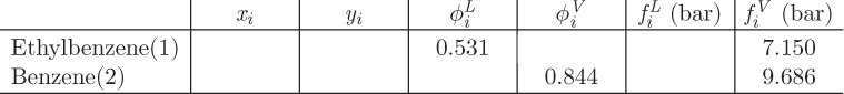
Problem 10.10: a) At 542 K, 21.7 bar, the system Ethylbenzene(1)/Benzene(2) is in vapor-liquid equilibrium. Available data for this system are given in the table below. Fill out the missing information on the table.
b) Calculate the entropy of a vapor mixture with y1 = 0.3 at 600 K, 12 bar. The reference state for each pure component is the ideal-gas state at 600 K, 12 bar. Additional information for part b: The residual entropy of the mixture at 600 K, 12 bar, is −1.8 J/mol K; the ideal-gas heat capacities of the pure components are CP1 = 120 J/mol K, CP2 = 150 J/mol K.
Problem 10.11: The binary system CO2 (1) normal pentane (2) can be described by the SRK equation with k12 = 0.12. Use this equation of state to do the following:
a) Compute and plot the Pxy graph of this system at 290 K. Annotate the graph properly. Show the tie line at 40 bar.
b) What is the phase of a mixture that contains 80% CO2 by mol at 40 bar? If a two-phase system, report the composition (x1, y1) and molar fractions (V, L) of the two phases.
c) Compute and plot the Txy graph for this system at 40 bar. Show the tie line at 290 K.
d) How much heat (kJ/mol) is needed to boil a saturated liquid with x1 = 0.8 under constant pressure P = 40 bar to produce saturated vapor?
e) A flow stream (x1 = 0.8) is compressed in an adiabatic compressor whose efficiency is 100%. The inlet is at 1 bar, 290 K and the outlet is delivered at 40 bar. Calculate the work for the compression (kJ/mol) as well as the temperature of the exit stream.
Problem 10.12: Use the SRK equation to calculate the Pxy graph of carbon dioxide (1)/normal pentane at 250 K. For this system k12 = 0.12.
a) Plot the Pxy graph at 250 K.
b) A stream contains a mixture of the two components with overall composition z1 = 50%. The conditions are 15 bar, 250 K. What is the phase of the system?
c) The above stream is flashed isothermally to a pressure such that the vapor contains 90% carbon dioxide. Determine the pressure and the concentration of CO2 in the liquid.
Problem 10.13: Use the SRK equation to compute a Txy graph for the system carbon dioxide (1)/normal pentane at 25 bar. Assume that k12 = 0.12 and independent of temperature.
a) Plot the Txy graph.
b) A saturated vapor-liquid stream at 25 bar with the overall composition z1 = 0.5 contains 50% vapor. What are the compositions of the two phases?
c) The stream passes through a heat exchanger where it is heated until the dew point is reached. What is the temperature?
d) How much heat is exchanged in the previous step?
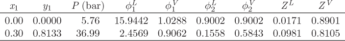
Problem 10.14: The table below gives data for the system hydrogen sulfide (1) in benzene (2) at 150 °C, using Peng-Robinson equation with k12 = 0.015.
a) Do you expect this system to exhibit a critical point at 150 °C?
b) Determine whether the solution behavior of benzene may be considered ideal in the concentration range x1 = 0 to 0.30.
c) Explain why the fugacity coefficients of benzene in the liquid and in the vapor are equal at 5.76 bar but different at 36.99 bar.