
5. Customer Profitability
Introduction
Chapter 2, “Share of Hearts, Minds, and Markets,” presented metrics designed to measure how well the firm is doing with its customers as a whole. Previously discussed metrics were summaries of firm performance with respect to customers for entire markets or market segments. In this chapter, we cover metrics that measure the performance of individual customer relationships. We start with metrics designed to simply count how many customers the firm serves. As this chapter will illustrate, it is far easier to count the number of units sold than to count the number of people or businesses buying those units. Section 5.2 introduces the concept of customer profit. Just as some brands are more profitable than others, so too are some customer relationships. Whereas customer profit is a metric that summarizes the past financial performance of a customer relationship, customer lifetime value looks forward in an attempt to value existing customer relationships. Section 5.3 discusses how to calculate and interpret customer lifetime value. One of the more important uses of customer lifetime value is to inform prospecting decisions. Section 5.4 explains how this can be accomplished and draws the careful distinction between prospect and customer value. Section 5.5 discusses acquisition and retention spending—two metrics firms track in order to monitor the performance of these two important kinds of marketing spending—spending designed to acquire new customers and spending designed to retain and profit from existing customers.

5.1 Customers, Recency, and Retention
A customer is a person or business that buys from the firm.
• Customer Counts: These are the number of customers of a firm for a specified time period.
• Recency: This refers to the length of time since a customer’s last purchase. A six-month customer is someone who purchased from the firm at least once within the last six months.
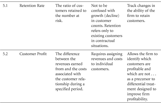
• Retention Rate: This is the ratio of the number of retained customers to the number at risk.
In contractual situations, it makes sense to talk about the number of customers currently under contract and the percentage retained when the contract period runs out.
In non-contractual situations (such as catalog sales), it makes less sense to talk about the current number of customers, but instead to count the number of customers of a specified recency.
Purpose: To monitor firm performance in attracting and retaining customers.
Only recently have most marketers worried about developing metrics that focus on individual customers. In order to begin to think about managing individual customer relationships, the firm must first be able to count its customers. Although consistency in counting customers is probably more important than formulating a precise definition, a definition is needed nonetheless. In particular, we think the definition of and the counting of customers will be different in contractual versus non-contractual situations.
Construction
Counting Customers
In contractual situations, it should be fairly easy to count how many customers are currently under contract at any point in time. For instance, Vodafone Australia,1 a global mobile phone company, was able to report 2.6 million direct customers at the end of the December quarter.
One complication in counting customers in contractual situations is the handling of contracts that cover two or more individuals. Does a family plan that includes five phones but one bill count as one or five? Does a business-to-business contract with one base fee and charges for each of 1,000 phones in use count as one or 1,000 customers? Does the answer to the previous question depend on whether the individual users pay Vodafone, pay their company, or pay nothing? In situations such as these, the firm must select some standard definition of a customer (policy holder, member) and implement it consistently.
A second complication in counting customers in contractual situations is the treatment of customers with multiple contracts with a single firm. USAA, a global insurance and diversified financial services association, provides insurance and financial services to the U.S. military community and their families. Each customer is considered a member, complete with a unique membership number. This allows USAA to know exactly how many members it has at any time—more than five million at the end of 2004—most of whom avail themselves of a variety of member services.
For other financial services companies, however, counts are often listed separately for each line of business. The 2003 annual report for State Farm Insurance, for example, lists a total of 73.9 million policies and accounts with a pie chart showing the percentage breakdown among auto, homeowners, life, annuities, and so on. Clearly the 73.9 million is a count of policies and not customers. Presumably because some customers use State Farm for auto, home, and life insurance, they get double and even triple counted in the 73.9 million number. Because State Farm knows the names and addresses of all their policyholders, it seems feasible that they could count how many individual customers they serve. The fact that State Farm counts policies and not customers suggests an emphasis on selling policies rather than managing customer relationships.
Finally, we offer an example of a natural gas company that went out of its way to double count customers—defining a customer to be “a consumer of natural gas distributed in any one billing period at one location through one meter. An entity using gas at separate locations is considered a separate customer at each location.” For this natural gas company, customers were synonymous with meters. This is probably a great way to view things if your job is to install and service meters. It is not such a great way to view things if your job is to market natural gas.
In non-contractual situations, the ability of the firm to count customers depends on whether individual customers are identifiable. If customers are not identifiable, firms can only count visits or transactions. Because Wal-Mart does not identify its shoppers, its customer counts are nothing more than the number of transactions that go through the cash registers in a day, week, or year. These “traffic” counts are akin to turnstile numbers at sporting events and visits to a Web site. In one sense they count people, but when summed over several periods, they no longer measure separate individuals. So whereas home attendance at Atlanta Braves games in 19932 was 3,884,720, the number of people attending one or more Braves games that year was some smaller number.
In non-contractual situations with identifiable customers (direct mail, retailers with frequent shopper cards, warehouse clubs, purchases of rental cars and lodging that require registration), a complication is that customer purchase activity is sporadic. Whereas the New York Times knows exactly how many current customers (subscribers) it has, the sporadic buying of cataloger L.L.Bean’s customers means that it makes no sense to talk about the number of current L.L.Bean customers. L.L.Bean will know the number of orders it receives daily, it will know the number of catalogs it mails monthly, but it cannot be expected to know the number of current customers it has because it is difficult to define a “current” customer.
Instead, firms in non-contractual situations count how many customers have bought within a certain period of time. This is the concept of recency—the length of time since the last purchase. Customers of recency one year or less are customers who bought within the last year. Firms in non-contractual situations with identifiable customers will count customers of various recencies.
Recency: The length of time since a customer’s last purchase.
For example, eBay reported 60.5 million active users in the first quarter of 2005. Active users were defined as the number of users of the eBay platform who bid, bought, or listed an item within the previous 12-month period. They go on to report that 45.1 million active users were reported in the same period a year ago.
Notice that eBay counts “active users” rather than “customers” and uses the concept of recency to track its number of active users across time. The number of active (12-month) users increased from 45.1 million to 60.5 million in one year. This tells the firm that the number of active customers increased due in part to customer acquisition. A measure of how well the firm maintained existing customer relationships is the percentage of the 45.1 million active customers one year ago who were active in the previous 12 months. That ratio measure is similar to retention in that it reflects the percentage of active customers who remained active in the subsequent period.
Retention: Applies to contractual situations in which customers are either retained or not. Customers either renew their magazine subscriptions or let them run out. Customers maintain a checking account with a bank until they close it out. Renters pay rent until they move out. These are examples of pure customer retention situations where customers are either retained or considered lost for good.
In these situations, firms pay close attention to retention rates.
Retention Rate: The ratio of the number of customers retained to the number at risk.
If 40,000 subscriptions to Fortune magazine are set to expire in July and the publisher convinces 26,000 of those customers to renew, we would say that the publisher retained 65% of its subscribers.
The complement of retention is attrition or churn. The attrition or churn rate for the 40,000 Fortune subscribers was 35%.
Notice that this definition of retention is a ratio of the number retained to the number at risk (of not being retained). The key feature of this definition is that a customer must be at risk of leaving in order to be counted as a customer successfully retained. This means that new Fortune subscribers obtained during July are not part of the equation, nor are the large number of customers whose subscriptions were set to run out in later months.
Finally, we point out that it sometimes makes better sense to measure retention in “customer time” rather than “calendar time.” Rather than ask what the firm’s retention rate was in 2004, it may be more informative to ask what percentage of customers surviving for three years were retained throughout year four.
Data Sources, Complications, and Cautions
The ratio of the total number of customers at the end of the period to the number of customers at the beginning of the period is not a retention rate. Retention during the period does affect this ratio, but customer acquisitions also affect the ratio.
The percentage of customers starting the period who remained customers throughout the period is a lot closer to being a retention rate. This percentage would be a true retention rate if all the customers starting the period were at risk of leaving during the period.
5.2 Customer Profit
Calculating customer profitability is an important step in understanding which customer relationships are better than others. Often, the firm will find that some customer relationships are unprofitable. The firm may be better off (more profitable) without these customers. At the other end, the firm will identify its most profitable customers and be in a position to take steps to ensure the continuation of these most profitable relationships.
Purpose: To identify the profitability of individual customers.
Companies commonly look at their performance in aggregate. A common phrase within a company is something like: “We had a good year, and the business units delivered $400,000 in profits.” When customers are considered, it is often using an average such as “We made a profit of $2.50 per customer.” Although these can be useful metrics, they sometimes disguise an important fact that not all customers are equal and, worse yet, some are unprofitable. Simply put, rather than measuring the “average customer,” we can learn a lot by finding out what each customer contributes to our bottom line.4
Customer Profitability: The difference between the revenues earned from and the costs associated with the customer relationship during a specified period.
The overall profitability of the company can be improved by treating dissimilar customers differently.
In essence, think of three different tiers of customer:
1. Top Tier customers—REWARD: Your most valuable customers are the ones you most want to retain. They should receive more of your attention than any other group. If you lose these guys, your profit suffers the most. Look to reward them in ways other than simply lowering your price. These customers probably value what you do the most and may not be price-sensitive.
2. Second Tier customers—GROW: The customers in the middle—with middle to low profits associated with them—might be targeted for growth. Here you have customers whom you may be able to develop into Top Tier customers. Look to the share of customer metrics described in Section 5.3 to help figure out which customers have the most growth potential.
3. Third Tier customers—FIRE: The company loses money on servicing these people. If you cannot easily promote them to the higher tiers of profitability, you should consider charging them more for the services they currently consume. If you can recognize this group beforehand, it may be best not to acquire these customers in the first place.
A database that can analyze the profitability of customers at an individual level can be a competitive advantage. If you can figure out profitability by customer, you have a chance to defend your best customers and maybe even poach the most profitable consumers from your competitors.
Construction
In theory, this is a trouble-free calculation. Find out the cost to serve each customer and the revenues associated with each customer for a given period. Do the subtraction to get profit for the customer and sort the customers based on profit. Although painless in theory, large companies with a multitude of customers will find this a major challenge even with the most sophisticated of databases.
To do the analysis with large databases, it may be necessary to abandon the notion of calculating profit for each individual customer and work with meaningful groups of customers instead.
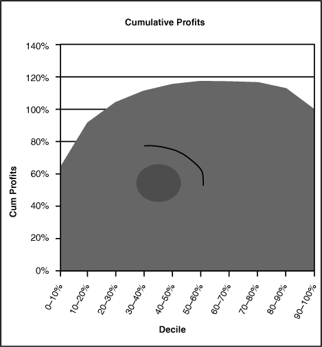
After you have the sorted list of customer profits (or customer-group profits), the custom is to plot cumulative percentage of total profits versus cumulative percentage of total customers. Given that the customers are sorted from highest to lowest profit, the resulting graph usually looks something like the head of a whale.
Profitability will increase sharply and tail off from the very beginning. (Remember, our customers have been sorted from most to least profitable.) Whenever there are some negative profit customers, the graph reaches a peak—above 100%—as profit per customer moves from positive to negative. As we continue through the negative-profit customers, cumulative profits decrease at an ever-increasing rate. The graph always ends at 100% of the customers accounting for 100% of the total profit.
Robert Kaplan (co-developer of Activity-Based Costing and the Balanced Scorecard) likes to refer to these curves as “whale curves.”5 In Kaplan’s experience, the whale curve usually reveals that the most profitable 20% of customers can sometimes generate between 150% and 300% of total profits so that the resulting curve resembles a sperm whale rising above the water’s surface. See Figure 5.2 for an example of a whale curve.
EXAMPLE: A catalog retailer has grouped customers in 10 deciles based on profitability (see Table 5.1 and Figure 5.1). (A decile is a tenth of the population, so 0-10% is the most profitable 10% of customers.)
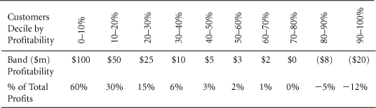
Table 5.1 Customer Profitability Ranked by Profitability
Here we have a clear illustration that if they were no longer to serve the least profitable 20% of customers, they would be $28 million better off.
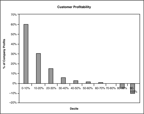
Figure 5.1 Customer Profitability by Decile

Table 5.2 Cumulative Profitability Peaks Before All Customers Are Served
Table 5.2 presents this same customer information in cumulative form. Cumulative profits plotted across deciles begins to look like a whale with a steeply rising ridge reaching a peak of total profitability above 100% and tapering off thereafter (see Figure 5.2).
Data Sources, Complications, and Cautions
Measuring customer profitability requires detailed information. Assigning revenues to customers is often the easy part; assigning your costs to customers is much harder. The cost of goods sold obviously gets assigned to the customers based on the goods each customer purchased. Assigning the more indirect costs may require the use of some form of activity-based costing (ABC) system. Finally, there may be some categories of costs that will be impossible to assign to the customer. If so, it is probably best to keep these costs as company costs and be content with the customer profit numbers adding up to something less than the total company profit.
When considering the profits from customers, it must be remembered that most things change over time. Customers who were profitable last year may not be profitable this year. Because the whale curve reflects past performance, we must be careful when using it to make decisions that shape the future. For example, we may very well want to continue a relationship that was unprofitable in the past if we know things will change for the better in the future. For example, banks typically offer discount packages to students to gain their business. This may well show low or negative customer profits in the short term. The “plan” is that future profits will compensate for current losses. Customer lifetime value (addressed in Section 5.3) is a forward-looking metric that attempts to account for the anticipated future profitability of each customer relationship.
When capturing customer information to decide which customers to serve, it is important to consider the legal environment in which the company operates. This can change considerably across countries, where there may be anti-discrimination laws and special situations in some industries. For instance, public utilities are sometimes obligated to serve all customers.
It is also worth remembering that intrusive capturing of customer-specific data can damage customer relationships. Some individuals will be put off by excess data gathering. For a food company, it may help to know which of your customers are on a diet. But the food company’s management should think twice before adding this question to their next customer survey.
Sometimes there are sound financial reasons for continuing to serve unprofitable customers. For example, some companies rely on network effects. Take the case of the United States Postal Service—part of its strength is the ability to deliver to the whole country. It may superficially seem profitable to stop deliveries to remote areas. But when that happens, the service becomes less valuable for all customers. In short, sometimes unprofitable customer relationships are necessary for the firm to maintain their profitable ones.
Similarly, companies with high fixed costs that have been assigned to customers during the construction of customer profit must ask whether those costs will go away if they terminate unprofitable customer relationships. If the costs do not go away, ending unprofitable relationships may only serve to make the surviving relationships look even less profitable (after the reallocation of costs) and result in the lowering of company profits. In short, make certain that the negative profit goes away if the relationship is terminated. Certainly the revenue and cost of goods sold will go away, but if some of the other costs do not, the firm could be better off maintaining a negative profit relationship as it contributes to covering fixed cost (refer to Sections 3.4 and 3.6).
Abandoning customers is a very sensitive practice, and a business should always consider the public relations consequences of such actions. Similarly, when you get rid of a customer, you cannot expect to attract them back very easily should they migrate into your profitable segment.
Finally, because the whale curve examines cumulative percentage of total profits, the numbers are very sensitive to the dollar amount of total profit. When the total dollar profit is a small number, it is fairly easy for the most profitable customers to represent a huge percentage of that small number. So when you hear that 20% of the firm’s customers represent 350% of the firm’s profit, one of the first things you should consider is the total dollar value of profits. If that total is small, 350% of it can also be a fairly small number of dollars. To cement this idea, ask yourself what the whale curve would look like for a firm with $0 profit.
5.3 Customer Lifetime Value
When margins and retention rates are constant, the following formula can be used to calculate the lifetime value of a customer relationship:
Customer lifetime value (CLV) is an important concept in that it encourages firms to shift their focus from quarterly profits to the long-term health of their customer relationships. Customer lifetime value is an important number because it represents an upper limit on spending to acquire new customers.
Purpose: To assess the value of each customer.
As Don Peppers and Martha Rogers are fond of saying, “some customers are more equal than others.”6 We saw a vivid illustration of this in the last section, which examined the profitability of individual customer relationships. As we noted, customer profit (CP) is the difference between the revenues and the costs associated with the customer relationship during a specified period. The central difference between CP and customer lifetime value (CLV) is that CP measures the past and CLV looks forward. As such, CLV can be more useful in shaping managers’ decisions but is much more difficult to quantify. Quantifying CP is a matter of carefully reporting and summarizing the results of past activity, whereas quantifying CLV involves forecasting future activity.
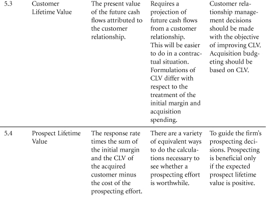
Customer Lifetime Value (CLV): The present value of the future cash flows attributed to the customer relationship.
The concept of present value will be talked about in more detail in Section 10.4. For now, you can think of present value as the discounted sum of future cash flows. We discount (multiply by a carefully selected number less than one) future cash flows before we add them together to account for the fact that there is a time value of money. The time value of money is another way of saying that everyone would prefer to get paid sooner rather than later and everyone would prefer to pay later rather than sooner. This is true for individuals (the sooner I get paid, the sooner I can pay down my credit card balance and avoid interest charges) as well as for firms. The exact discount factors used depend on the discount rate chosen (10% per year as an example) and the number of periods until we receive each cash flow (dollars received 10 years from now must be discounted more than dollars received five years in the future).
The concept of CLV is nothing more than the concept of present value applied to cash flows attributed to the customer relationship. Because the present value of any stream of future cash flows is designed to measure the single lump sum value today of the future stream of cash flows, CLV will represent the single lump sum value today of the customer relationship. Even more simply, CLV is the dollar value of the customer relationship to the firm. It is an upper limit on what the firm would be willing to pay to acquire the customer relationship as well as an upper limit on the amount the firm would be willing to pay to avoid losing the customer relationship. If we view a customer relationship as an asset of the firm, CLV would present the dollar value of that asset.
Cohort and Incubate
One way to project the value of future customer cash flows is to make the heroic assumption that the customers acquired several periods ago are no better or worse (in terms of their CLV) than the ones we currently acquire. We then go back and collect data on a cohort of customers all acquired at about the same time and carefully reconstruct their cash flows over some finite number of periods. The next step is to discount the cash flows for each customer back to the time of acquisition to calculate that customer’s sample CLV and then average all of the sample CLVs together to produce an estimate of the CLV of each newly acquired customer. We refer to this method as the “cohort and incubate” approach. Equivalently, one can calculate the present value of the total cash flows from the cohort and divide by the number of customers to get the average CLV for the cohort. If the value of customer relationships is stable across time, the average CLV of the cohort sample is an appropriate estimator of the CLV of newly acquired customers.
As an example of this cohort and incubate approach, Berger, Weinberg, and Hanna (2003) followed all the customers acquired by a cruise-ship line in 1993. The 6,094 customers in the cohort of 1993 were tracked (incubated) for five years. The total net present value of the cash flows from these customers was $27,916,614. These flows included revenues from the cruises taken (the 6,094 customers took 8,660 cruises over the five-year horizon), variable cost of the cruises, and promotional costs. The total five-year net present value of the cohort expressed on a per-customer basis came out to be $27,916,614/6,094 or $4,581 per customer. This is the average five-year CLV for the cohort.
“Prior to this analysis, [cruise-line] management would never spend more than $3,314 to acquire a passenger … Now, aware of CLV (both the concept and the actual numerical results), an advertisement that [resulted in a cost per acquisition of $3 to $4 thousand] was welcomed—especially because the CLV numbers are conservative (again, as noted, the CLV does not include any residual business after five years.)”7
The cohort and incubate approach works well when customer relationships are stationary—changing slowly over time. When the value of relationships changes slowly, we can use the value of incubated past relationships as predictive of the value of new relationships.
In situations where the value of customer relationships changes more rapidly, firms often use a simple model to forecast the value of those relationships. By a model, we mean some assumptions about how the customer relationship will unfold. If the model is simple enough, it may even be possible to find an equation for the present value of our model of future cash flows. This makes the calculation of CLV even easier because it now requires only the substitution of numbers for our situation into the equation for CLV.
Next, we will explain what is perhaps the simplest model for future customer cash flows and the equation for the present value of those cash flows. Although it’s not the only model of future customer cash flows, this one gets used the most.
Construction
The model for customer cash flows treats the firm’s customer relationships as something of a leaky bucket. Each period, a fraction (1 less the retention rate) of the firm’s customers leave and are lost for good.
The CLV model has only three parameters: 1) constant margin (contribution after deducting variable costs including retention spending) per period, 2) constant retention probability per period, and 3) discount rate. Furthermore, the model assumes that in the event that the customer is not retained, they are lost for good. Finally, the model assumes that the first margin will be received (with probability equal to the retention rate) at the end of the first period.
The one other assumption of the model is that the firm uses an infinite horizon when it calculates the present value of future cash flows. Although no firm actually has an infinite horizon, the consequences of assuming one are discussed in the following.
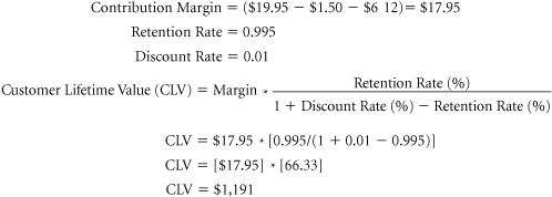
Customer Lifetime Value: The CLV formula8 multiplies the per-period cash margin (hereafter we will just use the term “margin”) by a factor that represents the present value of the expected length of the customer relationship:
Under the assumptions of the model, CLV is a multiple of the margin. The multiplicative factor represents the present value of the expected length (number of periods) of the customer relationship. When retention equals 0, the customer will never be retained, and the multiplicative factor is zero. When retention equals 1, the customer is always retained, and the firm receives the margin in perpetuity. The present value of the margin in perpetuity turns out to be Margin/Discount Rate. For retention values in between, the CLV formula tells us the appropriate multiplier.
EXAMPLE: An Internet Service Provider (ISP) charges $19.95 per month. Variable costs are about $1.50 per account per month. With marketing spending of $6 per year, their attrition is only 0.5% per month. At a monthly discount rate of 1%, what is the CLV of a customer?
Data Sources, Complications, and Cautions
The retention rate (and by extension the attrition rate) is a driver of customer value. Very small changes can make a major difference to the lifetime value calculated. Accuracy in this parameter is vital to meaningful results.
The retention rate is assumed to be constant across the life of the customer relationship. For products and services that go through a trial, conversion, and loyalty progression, retention rates will increase over the lifetime of the relationship. In those situations, the model explained here might be too simple. If the firm wants to estimate a sequence of retention rates, a spreadsheet model might be more useful in calculating CLV.
The discount rate is also a sensitive driver of the lifetime value calculation—as with retention, seemingly small changes can make major differences to customer lifetime value. The discount rate should be chosen with care.
The contribution is assumed to be constant across time. If margin is expected to increase over the lifetime of the customer relationship, the simple model will not apply.
Take care not to use this CLV formula for relationships in which customer inactivity does not signal the end of the relationship. In catalog sales, for example, a small percentage of the firm’s customers purchase from any given catalog. Don’t confuse the percentage of customers active in a given period (relevant for the cataloger) with the retention rates in this model. If customers often return to do business with the firm after a period of inactivity, this CLV formula does not apply.
Customer Lifetime Value (CLV) with Initial Margin: One final source of confusion concerns the timing assumptions inherent in the model. The first cash flow accounted for in the model is the margin received at the end of one period with probability equal to the retention rate. Other models also include an initial margin received at the beginning of the period. If a certain receipt of an initial margin is included, the new CLV will equal the old CLV plus the initial margin. Furthermore, if the initial margin is equal to all subsequent margins, there are at least two ways to write formulas for the CLV that include the initial margin:
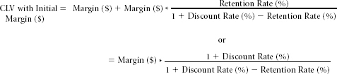
The second formula looks just like the original formula with 1 + Discount Rate taking the place of the retention rate in the numerator of the multiplicative factor. Just remember that the new CLV formula and the original CLV formula apply to the same situations and differ only in the treatment of an initial margin. This new CLV formula includes it, whereas the original CLV formula does not.
The Infinite Horizon Assumption
In some industries and companies it is typical to calculate four- or five-year customer values instead of using the infinite time horizon inherent in the previous formulas. Of course, over shorter periods customer retention rates are less likely to be affected by major shifts in technology or competitive strategies and are more likely to be captured by historical retention rates. For managers, the question is “Does it make a difference whether I use the infinite time horizon or (for example) the five-year customer value?” The answer to this question is yes, sometimes, it can make a difference because the value over five years can be less than 70% of the value over an infinite horizon (see Table 5.3).
Table 5.3 calculates the percentages of (infinite horizon) CLV accruing in the first five years. If retention rates are higher than 80% and discount rates are lower than 20%, differences in the two approaches will be substantial. Depending on the strategic risks that companies perceive, the additional complexities of using a finite horizon can be informative.
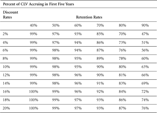
Table 5.3 Finite-Horizon CLV As a Percentage of Infinite-Horizon CLV
5.4 Prospect Lifetime Value Versus Customer Value
Only if prospect lifetime value is positive should the firm proceed with the planned acquisition spending.
Purpose: To account for the lifetime value of a newly acquired customer (CLV) when making prospecting decisions.
One of the major uses of CLV is to inform prospecting decisions. A prospect is someone whom the firm will spend money on in an attempt to acquire her or him as a customer. The acquisition spending must be compared not just to the contribution from the immediate sales it generates but also to the future cash flows expected from the newly acquired customer relationship (the CLV). Only with a full accounting of the value of the newly acquired customer relationship will the firm be able to make an informed, economic prospecting decision.
Construction
The expected prospect lifetime value (PLV) is the value expected from each prospect minus the cost of prospecting. The value expected from each prospect is the acquisition rate (the expected fraction of prospects who will make a purchase and become customers) times the sum of the initial margin the firm makes on the initial purchases and the CLV. The cost is the amount of acquisition spending per prospect. The formula for expected PLV is as follows:
Prospect Lifetime Value ($) = Acquisition Rate (%) * [Initial Margin ($) + CLV ($)] — Acquisition Spending ($)
If PLV is positive, the acquisition spending is a wise investment. If PLV is negative, the acquisition spending should not be made.
The PLV number will usually be very small. Although CLV is sometimes in the hundreds of dollars, PLV can come out to be only a few pennies. Just remember that PLV applies to prospects, not customers. A large number of small but positive-value prospects can add to a considerable amount of value for a firm.
EXAMPLE: A service company plans to spend $60,000 on an advertisement reaching 75,000 readers. If the service company expects the advertisement to convince 1.2% of the readers to take advantage of a special introductory offer (priced so low that the firm makes only $10 margin on this initial purchase) and the CLV of the acquired customers is $100, is the advertisement economically attractive?
Here Acquisition Spending is $0.80 per prospect, the expected acquisition rate is 0.012, and the initial margin is $10. The expected PLV of each of the 75,000 prospects is
The expected PLV is $0.52. The total expected value of the prospecting effort will be 75,000 * $0.52 = $39,000. The proposed acquisition spending is economically attractive.
If we are uncertain about the 0.012 acquisition rate, we might ask what the acquisition rate from the prospecting campaign must be in order for it to be economically successful. We can get that number using Excel’s goal seek function to find the acquisition rate that sets PLV to zero. Or we can use a little algebra and substitute $0 in for PLV and solve for the break-even acquisition rate:
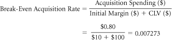
The acquisition rate must exceed 0.7273% in order for the campaign to be successful.
Data Sources, Complications, and Cautions
In addition to the CLV of the newly acquired customers, the firm needs to know the planned amount of acquisition spending (expressed on a per-prospect basis), the expected success rate (the fraction of prospects expected to become customers), and the average margin the firm will receive from the initial purchases of the newly acquired customers. The initial margin number is needed because CLV as defined in the previous section accounts for only the future cash flows from the relationship. The initial cash flow is not included in CLV and must be accounted for separately. Note also that the initial margin must account for any first-period retention spending.
Perhaps the biggest challenge in calculating PLV is estimating CLV. The other terms (acquisition spending, acquisition rate, and initial margin) all refer to flows or outcomes in the near future, whereas CLV requires longer-term projections.
Another caution worth mentioning is that the decision to spend money on customer acquisition whenever PLV is positive rests on an assumption that the customers acquired would not have been acquired had the firm not spent the money. In other words, our approach gives the acquisition spending “full credit” for the subsequent customers acquired. If the firm has several simultaneous acquisition efforts, dropping one of them might lead to increased acquisition rates for the others. Situations such as these (where one solicitation cannibalizes another) require a more complicated analysis.
The firm must be careful to search for the most economical way to acquire new customers. If there are alternative prospecting approaches, the firm must be careful not to simply go with the first one that gives a positive projected PLV. Given a limited number of prospects, the approach that gives the highest expected PLV should be used.
Finally, we want to warn you that there are other ways to do the calculations necessary to judge the economic viability of a given prospecting effort. Although these other approaches are equivalent to the one presented here, they differ with respect to what gets included in “CLV.” Some will include the initial margin as part of “CLV.” Others will include both the initial margin and the expected acquisition cost per acquired customer as part of “CLV.” We illustrate these two approaches using the service company example.
EXAMPLE: A service company plans to spend $60,000 on an advertisement reaching 75,000 readers. If the service company expects the advertisement to convince 1.2% of the readers to take advantage of a special introductory offer (priced so low that the firm makes only $10 margin on this initial purchase) and the CLV of the acquired customers is $100, is the advertisement economically attractive?
If we include the initial margin in “CLV” we get
The expected PLV is now
This is the same number as before calculated using a slightly different “CLV”—one that includes the initial margin.
We illustrate one final way to do the calculations necessary to judge the economics of a prospecting campaign. This last way does things on a per-acquired-customer basis using a “CLV” that includes both initial margin and an allocated acquisition spending. The thinking goes as follows: The expected value of a new customer is $10 now plus $100 from future sales, or $110 in total. The expected cost to acquire a customer is the total cost of the campaign divided by the expected number of new customers. This average acquisition cost is calculated as $60,000/(0.012 * 75,000) = $66.67. The expected value of a new customer net of the expected acquisition cost per customer is $110 — $66.67 = $43.33. Because this new “net” CLV is positive, the campaign is economically attractive. Some will even label this $43.33 number as the “CLV” of a new customer.
Notice that $43.33 times the 900 expected new customers equals $39,000, the same total net value from the campaign calculated in the original example as the $0.52 PLV times the 75,000 prospects. The two ways to do the calculations are equivalent.
5.5 Acquisition Versus Retention Cost

These two metrics help the firm monitor the effectiveness of two important categories of marketing spending.
Purpose: To determine the firm’s cost of acquisition and retention.
Before the firm can optimize its mix of acquisition and retention spending, it must first assess the status quo. At the current spending levels, how much does it cost the firm (on average) to acquire new customers, and how much is it spending (on average) to retain its existing customers? Does it cost five times as much to acquire a new customer as it does to retain an existing one?
Construction
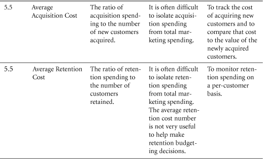
Average Acquisition Cost: This represents the average cost to acquire a customer and is the total acquisition spending divided by the number of new customers acquired.
Average Retention Cost: This represents the average “cost” to retain an existing customer and is the total retention spending divided by the number of customers retained.
Data Sources, Complications, and Cautions
For any specific period, the firm needs to know the total amount it spent on customer acquisition and the number of new customers that resulted from that spending. With respect to customer retention, the firm needs to measure the total amount spent during the period attempting to retain the customers in existence at the start of the period and the number of the existing customers successfully retained at the end of the period. Notice that retention spending directed at customers acquired within the period is not included in this figure. Similarly, the number retained refers only to those retained from the pool of customers in existence at the start of the period. Thus, the average retention cost calculated will be associated with the length of the period in question. If the period is a year, the average retention cost will be a cost per year per customer retained.
The calculation and interpretation of average acquisition cost is much easier than the calculation and interpretation of average retention cost. This is so because it is often possible to isolate acquisition spending and count the number of new customers that resulted from that spending. A simple division results in the average cost to acquire a customer. The reasonable assumption underlying this calculation is that the new customers would not have been acquired had it not been for the acquisition spending.
Things are not nearly so clear when it comes to average retention cost. One source of difficulty is that retention rates (and costs) depend on the period of time under consideration. Yearly retention is different from monthly retention. The cost to retain a customer for a month will be less than the cost to retain a customer for a year. Thus, the definition of average retention cost requires a specification of the time period associated with the retention.
A second source of difficulty stems from the fact that some customers will be retained even if the firm spends nothing on retention. For this reason it can be a little misleading to call the ratio of retention spending to the number of retained customers the average retention cost. One must not jump to the conclusion that retention goes away if the retention spending goes away. Nor should one assume that if the firm increases the retention budget by the average retention cost that it will retain one more customer. The average retention cost number is not very useful to help make retention budgeting decisions.
One final caution involves the firm’s capability to separate spending into acquisition and retention classifications. Clearly there can be spending that works to improve both the acquisition and retention efforts of the firm. General brand advertisements, for example, serve to lower the cost of both acquisition and retention. Rather than attempt to allocate all spending as either acquisition or retention, we suggest that it is perfectly acceptable to maintain a separate category that is neither acquisition nor retention.
References and Suggested Further Reading
Berger, Weinberg, and Hanna. (2003). “Customer Lifetime Value Determination and Strategic Implications for a Cruise-Ship Line,” Database Marketing and Customer Strategy Management, 11(1).
Blattberg, R.C., and S.J. Hoch. (1990). “Database Models and Managerial Intuition: 50% Model + 50% Manager,” Management Science, 36(8), 887–899.
Gupta, S., and Donald R. Lehmann. (2003). “Customers As Assets,” Journal of Interactive Marketing, 17(1).
Kaplan, R.S., and V.G. Narayanan. (2001). “Measuring and Managing Customer Profitability,” Journal of Cost Management, September/October: 5–15.
Little, J.D.C. (1970). “Models and Managers: The Concept of a Decision Calculus,” Management Science, 16(8), B-466; B-485.
McGovern, G.J., D. Court, JA. Quelch, and B. Crawford. (2004). “Bringing Customers into the Boardroom,” Harvard Business Review, 82(11), 70–80.
Much, J.G., Lee S. Sproull, and Michal Tamuz. (1989). “Learning from Samples of One or Fewer,” Organization Science: A Journal of the Institute of Management Sciences, 2(1), 1–12.
Peppers, D., and M. Rogers. (1997). Enterprise One-to-One: Tools for Competing in the Interactive Age (1st ed.), New York: Currency Doubleday.
Pfeifer, P.E., M.E. Haskins, and R.M. Conroy. (2005). “Customer Lifetime Value, Customer Profitability, and the Treatment of Acquisition Spending,” Journal of Managerial Issues, 17(1), 11–25.