
Chapter 13. Plates and Shells
13.1 Introduction
This chapter is subdivided into two parts. In Part A, we develop the governing equations and methods of solution of deflection for rectangular and circular plates. Applications of the energy and finite element methods for computation of deflection and stress in plates are also included. Membrane stresses in shells are taken up in Part B. Load-carrying mechanism of a shell, which differs from that of other elements, is demonstrated first. This is followed with a discussion of stress distribution in spherical, conical, and cylindrical shells. Thermal stresses in compound cylindrical shells are also considered.
Part A—Bending of Thin Plates
13.2 Basic Assumptions
Plates and shells are initially flat and curved structural elements, respectively, with thicknesses small compared with the remaining dimensions. We first consider plates, for which it is usual to divide the thickness t into equal halves by a plane parallel to the faces. This plane is termed the midsurface of the plate. The plate thickness is measured in a direction normal to the midsurface at each point under consideration. Plates of technical significance are often defined as thin when the ratio of the thickness to the smaller span length is less than 1/20. We here treat the small deflection theory of homogeneous, uniform thin plates, leaving for the numerical approach of Section 13.10 a discussion of plates of nonuniform thickness and irregular shape.
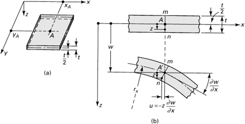
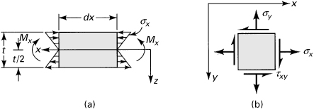
Consider now a plate prior to deformation, shown in Fig. 13.1a, in which the xy plane coincides with the midsurface and hence the z deflection is zero. When, owing to external loading, deformation occurs, the midsurface at any point xA, yA suffers a deflection w. Referring to the coordinate system shown, the fundamental assumptions of the small deflection theory of bending for isotropic, homogeneous, thin plates may be summarized as follows:
1. The deflection of the midsurface is small in comparison with the thickness of the plate. The slope of the deflected surface is much less than unity.
2. Straight lines initially normal to the midsurface remain straight and normal to that surface subsequent to bending. This is equivalent to stating that the vertical shear strains γxz and γyz are negligible. The deflection of the plate is thus associated principally with bending strains, with the implication that the normal strain εz owing to vertical loading may also be neglected.
3. No midsurface straining or in-plane straining, stretching, or contracting occurs as a result of bending.
4. The component of stress normal to the midsurface, σz, is negligible.
Figure 13.1. Deformation of a plate in bending.
These presuppositions are analogous to those associated with simple bending theory of beams.
13.3 Strain–Curvature Relations
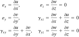
We here develop fundamental relationships between the strains and curvatures of the midsurface of thin plates. On the basis of assumption 2 stated in the preceding section, the strain–displacement relations of Eq. (2.4) reduce to
Integration of εz = ∂w/∂z = 0 yields
(13.1)
indicating that the lateral deflection does not vary throughout the plate thickness. Similarly, integrating the expressions for γxz and γyz, we obtain
(b)
It is clear that f2(x, y) and f3(x, y) represent, respectively, the values of u and v corresponding to z = 0 (the midsurface). Because assumption 3 precludes such in-plane straining, we conclude that f2 = f3 = 0, and therefore
(13.2)
where ∂w/∂x and ∂w/∂y are the slopes of the midsurface. The expression for u is represented in Fig. 13.1b at section mn passing through arbitrary point A(xA, yA). A similar interpretation applies for v in the zy plane. It is observed that Eqs. (13.2) are consistent with assumption 2. Combining the first three equations of (a) with Eq. (13.2), we have
(13.3a)
which provide the strains at any point.
Because in small deflection theory the square of a slope may be regarded as negligible, the partial derivatives of Eqs. (13.3a) represent the curvatures of the plate (see Eq. 5.7). Therefore, the curvatures at the midsurface in planes parallel to the xz (Fig. 13.1b), yz, and xy planes are, respectively,
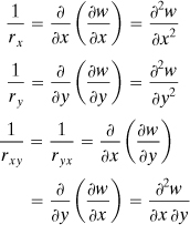
(13.4)
The foregoing are simply the rates at which the slopes vary over the plate.
In terms of the radii of curvature, the strain–deflection relations (13.3a) may be written
(13.3b)
Examining these equations, we are led to conclude that a circle of curvature can be constructed similarly to Mohr’s circle of strain. The curvatures therefore transform in the same manner as the strains. It can be verified by employing Mohr’s circle that (1/rx) + (1/ry) = ∇2w. The sum of the curvatures in perpendicular directions, called the average curvature, is invariant with respect to rotation of the coordinate axis. This assertion is valid at any location on the midsurface.
13.4 Stress, Curvature, and Moment Relations
The stress components σx, σy, and τxy = τyx are related to the strains by Hooke’s law, which for a thin plate becomes
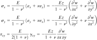
(13.5)
These expressions demonstrate clearly that the stresses vanish at the midsurface and vary linearly over the thickness of the plate.
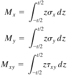
The stresses distributed over the side surfaces of the plate, while producing no net force, do result in bending and twisting moments. These moment resultants per unit length (for example, newtons times meters divided by meters, or simply newtons) are denoted Mx, My, and Mxy. Referring to Fig. 13.2a,
Figure 13.2. (a) Plate segment in pure bending; (b) positive stresses on an element in the bottom half of a plate.
Expressions involving My and Mxy = Myx are similarly derived. The bending and twisting moments per unit length are thus
(13.6)
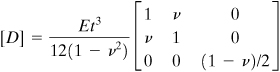
Introducing into Eq. (13.6) the stresses given by Eqs. (13.5), and taking into account the fact that w = w(x, y), we obtain
(13.7)
where
(13.8)
is the flexural rigidity of the plate. Note that, if a plate element of unit width were free to expand sidewise under the given loading, anticlastic curvature would not be prevented; the flexural rigidity would be Et3/12. The remainder of the plate does not permit this action, however. Because of this, a plate manifests greater stiffness than a narrow beam by a factor 1/(1 – ν2) or about 10%. Under the sign convention, a positive moment is one that results in positive stresses in the positive (bottom) half of the plate (Sec. 1.5), as shown in Fig. 13.2b.
Substitution of z = t/2 into Eq. (13.5), together with the use of Eq. (13.7), provides expressions for the maximum stress (which occurs on the surface of the plate):
(13.9)
Employing a new set of coordinates in which x′, y′ replaces x, y and z′ = z, we first transform σx, σy, τxy into σx′, σy′, τx′y′ through the use of Eq. (1.18). These are then substituted into Eq. (13.6) to obtain the corresponding Mx′, My′, Mx′y′. Examination of Eqs. (13.6) and (13.9) indicates a direct correspondence between the moments and stresses. It is concluded, therefore, that the equation for transforming the stresses should be identical with that used for the moments. Mohr’s circle may thus be applied to moments as well as to stresses.
13.5 Governing Equations of Plate Deflection
Consider now a plate element dx dy subject to a uniformly distributed lateral load per unit area p (Fig. 13.3). In addition to the moments Mx, My, and Mxy previously discussed, we now find vertical shearing forces Qx and Qy (force per unit length) acting on the sides of the element. These forces are related directly to the vertical shearing stresses:
(13.10)
Figure 13.3. Positive moments and shear forces (per unit length) and distributed lateral load (per unit area) on a plate element.
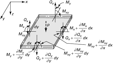
The sign convention associated with Qx and Qy is identical with that for the shearing stresses τxz and τyz: A positive shearing force acts on a positive face in the positive z direction (or on a negative face in the negative z direction). The bending moment sign convention is as previously given. On this basis, all forces and moments shown in Fig. 13.3 are positive.
It is appropriate to emphasize that while the simple theory of thin plates neglects the effect on bending of σz, γxz = τxz/G, and γyz = τyz/G (as discussed in Sec. 13.2), the vertical forces Qx and Qy resulting from τxz and τyz are not negligible. In fact, they are of the same order of magnitude as the lateral loading and moments.
It is our next task to obtain the equation of equilibrium for an element and eventually to reduce the system of equations to a single expression involving the deflection w. Referring to Fig. 13.3, we note that body forces are assumed negligible relative to the surface loading and that no horizontal shear and normal forces act on the sides of the element. The equilibrium of z-directed forces is governed by
or
(a)
For the equilibrium of moments about the x axis,
![]()
from which
(b)
Higher-order terms, such as the moment of p and the moment owing to the change in Qy, have been neglected. The equilibrium of moments about the y axis yields an expression similar to Eq. (b):
(c)
Equations (b) and (c), when combined with Eq. (13.7), lead to
(13.11)
Finally, substituting Eq. (13.11) into Eq. (a) results in the governing equation of plate theory (Lagrange, 1811):
(13.12a)
or, in concise form,
(13-12b)
The bending of plates subject to a lateral loading p per unit area thus reduces to a single differential equation. Determination of w(x, y) relies on the integration of Eq. (13.12) with the constants of integration dependent on the identification of appropriate boundary conditions. The shearing stresses τxz and τyz can be readily determined by applying Eqs. (13.11) and (13.10) once w(x, y) is known. These stresses display a parabolic variation over the thickness of the plate. The maximum shearing stress, as in the case of a beam of rectangular section, occurs at z = 0:
(13.13)
The key to evaluating all the stresses, employing Eqs. (13.5) or (13.9) and (13.3), is thus the solution of Eq. (13.12) for w(x, y). As already indicated, τxz and τyz are regarded as small compared with the remaining plane stresses.
13.6 Boundary Conditions
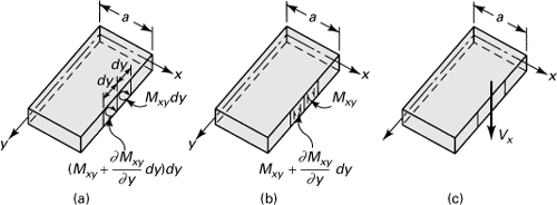
Solution of the plate equation requires that two boundary conditions be satisfied at each edge. These may relate to deflection and slope, or to forces and moments, or to some combination. The principal feature distinguishing the boundary conditions applied to plates from those applied to beams relates to the existence along the plate edge of twisting moment resultants. These moments, as demonstrated next, may be replaced by an equivalent vertical force, which when added to the vertical shearing force produces an effective vertical force.
Consider two successive elements of lengths dy on edge x = a of the plate shown in Fig. 13.4a. On the right element, a twisting moment Mxy dy acts, while the left element is subject to a moment [Mxy + (∂Mxy/∂y) dy]dy. In Fig. 13.4b, we observe that these twisting moments have been replaced by equivalent force couples that produce only local differences in the distribution of stress on the edge x = a. The stress distribution elsewhere in the plate is unaffected by this substitution. Acting at the left edge of the right element is an upward directed force Mxy. Adjacent to this force is a downward directed force Mxy + (∂Mxy/∂y) dy acting at the right edge of the left element. The difference between these forces (expressed per unit length), ∂Mxy/∂y, may be combined with the transverse shearing force Qx to produce an effective transverse edge force per unit length, Vx, known as Kirchhoff’s force (Fig. 13.4c):
![]()
Figure 13.4. Edge effect of twisting moment.
Substitution of Eqs. (13.7) and (13.11) into this leads to
(13.14)
We are now in a position to formulate a variety of commonly encountered situations. Consider first the conditions that apply along the clamped edge x = a of the rectangular plate with edges parallel to the x and y axes (Fig. 13.5a). As both the deflection and slope are zero,
(13.15)
Figure 13.5. Various boundary conditions: (a) fixed edge; (b) simple support; (c) free edge.
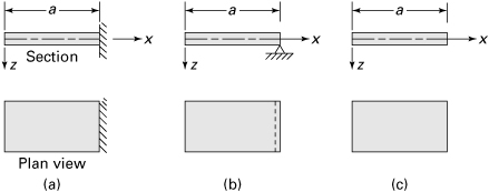
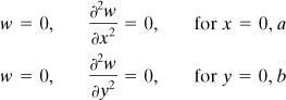
For the simply supported edge (Fig. 13.5b), the deflection and bending moment are both zero:
(13.16a)
Because the first of these equations implies that along edge x = a, ∂w/∂y = 0 and ∂2w/∂y2 = 0, the conditions expressed by Eq. (13.16a) may be restated in the following equivalent form:
(13.16b)
For the case of the free edge (Fig. 13.5c), the moment and vertical edge force are zero:
(13.17)
Example 13.1. Simply Supported Plate Strip
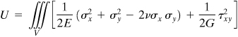
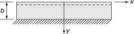
Derive the equation describing the deflection of a long and narrow plate, simply supported at edges y = 0 and y = b (Fig. 13.6). The plate is subjected to nonuniform loading
(a)
Figure 13.6. Example 13.1. A long and narrow simply supported plate.
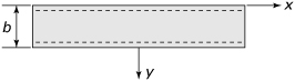
so that it deforms into a cylindrical surface with its generating line parallel to the x axis. The constant po thus represents the load intensity along the line passing through y = b/2, parallel to x.
Solution
Because for this situation ∂w/∂x = 0 and ∂2w/∂x∂y = 0, Eq. (13.7) reduces to
(b)
while Eq. (13.12) becomes
(c)
The latter expression is the same as the wide beam equation, and we conclude that the solution proceeds as in the case of a beam. A wide beam shall, in the context of this chapter, mean a rectangular plate supported on one edge or on two opposite edges in such a way that these edges are free to approach one another as deflection occurs.
Substituting Eq. (a) into Eq. (c), integrating, and satisfying the boundary conditions at y = 0 and y = b, we obtain
(d)
The stresses are now readily determined through application of Eqs. (13.5) or (13.9) and Eq. (13.13).
13.7 Simply Supported Rectangular Plates
In general, the solution of the plate problem for a geometry as in Fig. 13.7a, with simple supports along all edges, may be obtained by the application of Fourier series for load and deflection:*
(13.18a)
(13.18b)
Figure 13.7. Simply supported rectangular plate: (a) location of coordinate system for Navier’s method; (b) deflection of the simply supported plate into half-sine curves of m = 1 and n = 2.
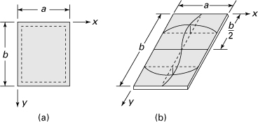
Here pmn and amn represent coefficients to be determined. The problem at hand is described by
(a)
(b)
The boundary conditions given are satisfied by Eq. (13.18b), and the coefficients amn must be such as to satisfy Eq. (a). The solution corresponding to the loading p(x, y) thus requires a determination of pmn and amn. Let us consider, as an interpretation of Eq. (13.18b), the true deflection surface of the plate to be the superposition of sinusoidal curves m and n different configurations in the x and y directions. The coefficients amn of the series are the maximum central coordinates of the sine series, and the m’s and the n’s mean the number of the half-sine curves in the x and y directions, respectively. For instance, the terms a a12 sin (πx/a) sin (2πy/b) of the series is shown in Fig. 13.7b. By increasing the number of terms in the series, the accuracy can be improved.
We proceed by dealing first with a general load configuration, subsequently treating specific loadings. To determine the coefficients pmn, each side of Eq. (13.18a) is multiplied by
![]()
Integrating between the limits 0, a and 0, b yields
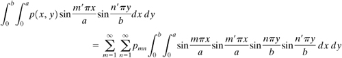
Applying the orthogonality relation (10.24) and integrating the right side of the preceding equation, we obtain
(13.19)
Evaluation of amn in Eq. (13.18b) requires substitution of Eqs. (13.18a) and (13.18b) into Eq. (a), with the result
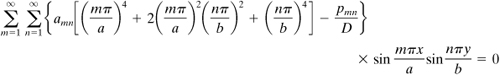
This expression must apply for all x and y; we conclude therefore that
(c)
Solving for amn and substituting into Eq. (13.18b), the equation of the deflection surface of a thin plate is
(13.20)
in which pmn is given by Eq. (13.19).
Example 13.2. Analysis of Uniformly Loaded Rectangular Plate
(a) Determine the deflections and moments in a simply supported rectangular plate of thickness t (Fig. 13.7a). The plate is subjected to a uniformly distributed load po. (b) Setting a = b, obtain the deflections, moments, and stresses in the plate.
Solution
a. For this case, p(x, y) = po, and Eq. (13.19) is thus
![]()
It is seen that, because pmn = 0 for even values of m and n, they can be taken as odd integers. Substituting pmn into Eq. (13.20) results in
(13.21)
We know that on physical grounds, the uniformly loaded plate must deflect into a symmetrical shape. Such a configuration results when m and n are odd. The maximum deflection occurs at x = a/2, y = b/2. From Eq. (13.21), we thus have
(13.22)
By substituting Eq. (13.21) into Eq. (13.7), the bending moments Mx, My are obtained:
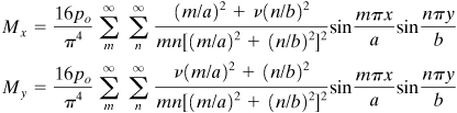
(13.23)
b. For the case of a square plate (setting a = b), substituting ν = 0.3, the first term of Eq. (13.22) gives
![]()
The rapid convergence of Eq. (13.22) is demonstrated by noting that retaining the first four terms gives the results wmax = 0.0443po(a4/Et3).
The bending moments occurring at the center of the plate are found from Eq. (13.23). Retaining only the first term, the result is
Mx, max = My, max = 0.0534poa2
while the first four terms yield
Mx, max = My, max = 0.0472poa2
Observe from a comparison of these values that the series given by Eq. (13.23) does not converge as rapidly as that of Eq. (13.22).
13.8 Axisymmetrically Loaded Circular Plates
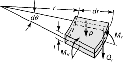
The deflection w of a circular plate will manifest dependence on radial position r only if the applied load and conditions of end restraint are independent of the angle θ. In other words, symmetry in plate deflection follows from symmetry in applied load. For this case, only radial and tangential moments Mr and Mθ per unit length and force Qr per unit length act on the circular plate element shown in Fig. 13.8. To derive the fundamental equations of a circular plate, we need only transform the appropriate formulations of previous sections from Cartesian to polar coordinates.
Figure 13.8. Axisymmetrically loaded circular plate element. (Only shear force and moments on the positive faces are shown.)
Through the application of the coordinate transformation relationships of Section 3.8, the bending moments and vertical shear forces are found from Eqs. (13.7) and (13.11) to be Qθ = 0, Mrθ = 0, and
(13.24b)
(13.24c)
The differential equation describing the surface deflection is obtained from Eq. (13.12) in a similar fashion:
(13.25a)
where p, as before, represents the load acting per unit of surface area, and D is the plate rigidity. By introducing the identity
(a)
Eq. (13.25a) assumes the form
(13.25b)
For applied loads varying with radius, p(r), representation (13.25b) is preferred.
The boundary conditions at the edge of the plate of radius a may readily be written by referring to Eqs. (13.15) to (13.17) and (13.24):
(13.26a)
(13.26b)
(13.26c)
Equation (13.25), together with the boundary conditions, is sufficient to solve the axisymmetrically loaded circular plate problem.
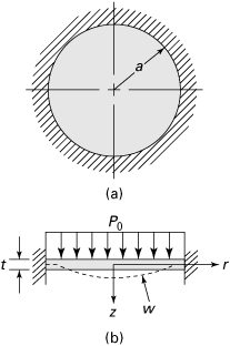
Example 13.3. Circular Plate with Fixed-Edge
Determine the stress and deflection for a built-in circular plate of radius a subjected to uniformly distributed loading po (Fig. 13.9).
Figure 13.9. Example 13.3. Uniformly loaded clamped circular plate: (a) top view; (b) front view.
Solution
The origin of coordinates is located at the center of the plate. The displacement w is obtained by successive integration of Eq. (13.25b):
![]()
or
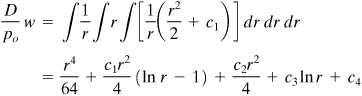
(b)
where the c’s are constants of integration.
The boundary conditions are
(c)
The terms involving logarithms in Eq. (b) lead to an infinite displacement at the center of the plate (r = 0) for all values of c1 and c3 except zero; therefore, c1 = c3 = 0. Satisfying the boundary conditions (c), we find that c2 = –a2/8 and c4 = a4/64. The deflection is then
(13.27)
The maximum deflection occurs at the center of the plate:
![]()
Substituting the deflection given by Eq. (13.27) into Eq. (13.24), we have
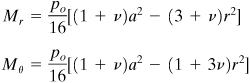
(13.28)
The extreme values of the moments are found at the center and edge. At the center,
![]()
At the edges, Eq. (13.28) yields
![]()
Examining these results, it is clear that the maximum stress occurs at the edge:
(13.29)
A similar procedure may be applied to symmetrically loaded circular plates subject to different end conditions.
13.9 Deflections of Rectangular Plates by the Strain-Energy Method
Based on the assumptions of Section 13.2, for thin plates, stress components σz, τxz, and τyz can be neglected. Therefore, the strain energy in pure bending of plates, from Eq. (2.52), has the form
(a)
Integration extends over the entire plate volume. For a plate of uniform thickness, this expression may be written in terms of deflection w, applying Eqs. (13.5) and (13.8), as follows:
(13.30)
(13.31)
where A is the area of the plate surface.
If the edges of the plate are fixed or simply supported, the second term on the right of Eq. (13.31) becomes zero [Ref. 13.1]. Hence, the strain energy simplifies to
(13.32)
The work done by the lateral load p is
(13.33)
The potential energy of the system is then
(13.34)
Application of a strain-energy method in calculating deflections of a rectangular plate is illustrated next.
Example 13.4. Deflection of a Rectangular Plate
Rework Example 13.2 using the Rayleigh–Ritz method.
Solution
From the discussion of Section 13.7, the deflection of the simply supported plate (Fig. 13.7a) can always be represented in the form of a double trigonometric series given by Eq. (13.18b). Introducing this series for w and setting p = po, Eq. (13.34) becomes
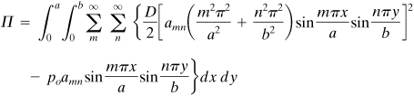
(b)
Observing the orthogonality relation [Eq. (10.24)], we conclude that, in calculating the first term of the preceding integral, we need to consider only the squares of the terms of the infinite series in the parentheses (Prob. 13.19). Hence, integrating Eq. (b), we have
(c)
From the minimizing conditions ∂Π/∂amn = 0, it follows that
(d)
Substitution of these coefficients into Eq. (13.18b) leads to the same expression as given by Eq. (13.21).
13.10 Finite Element Solution
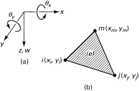
In this section we present the finite element method (Chapter 7) for computation of deflection, strain, and stress in a thin plate. For details, see, for example, Refs. 13.3 through 13.6. The plate, in general, may have any irregular geometry and loading. The derivations are based on the assumptions of small deformation theory, described in Section 13.2. A triangular plate element ijm coinciding with the xy plane will be employed as the finite element model (Fig. 13.10). Each nodal displacement of the element possesses three components: a displacement in the z direction, w; a rotation about the x axis, θx; and a rotation about the y axis, θy. Positive directions of the rotations are determined by the right-hand rule, as illustrated in the figure. It is clear that rotations θx and θy represent the slopes of w: ∂w/∂y and ∂w/∂x, respectively.
Figure 13.10. (a) Positive directions of displacements; (b) triangular finite plate element.
Strain, Stress, and Elasticity Matrices
Referring to Eqs. (13.3), we define, for the finite element analysis, a generalized “strain”-displacement matrix as follows:
(13.35)
The moment generalized “strain” relationship, from Eq. (13.7), is given in matrix form as
(13.36)
(13.37)
The stresses {σ}e and the moments {M}e are related by Eq. (13.9).
Displacement Function
The nodal displacement can be defined, for node i, as follows:
(a)
The element nodal displacements are expressed in terms of submatrices θi, θj, and θm:
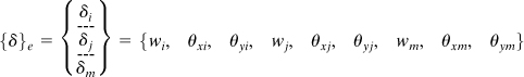
(b)
The displacement function {f} = w is assumed to be a modified third-order polynomial of the form
(c)
Note that the number of terms is the same as the number of nodal displacements of the element. This function satisfies displacement compatibility at interfaces between elements but does not satisfy the compatibility of slopes at these boundaries. Solutions based on Eq. (c) do, however, yield results of acceptable accuracy.
The constants a1 through a9 can be evaluated by writing the nine equations involving the values of w and θ at the nodes:
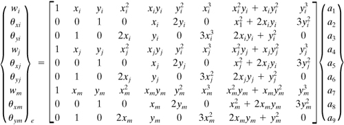
(13.38a)
or
(13.38b)
(13.39)
It is observed in Eq. (13.38) that the matrix [C] depends on the coordinate dimensions of the nodal points.
Note that the displacement function may now be written in the usual form of Eq. (7.50) as
(13.40)
in which
(13.41)
Introducing Eq. (c) into Eq. (13.35), we have
(13.42a)
or
(13.42b)
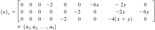
Upon substituting the values of the constants {a} from Eq. (13.39) into (13.42b), we can obtain the generalized “strain”–displacement matrix in the following common form:
{ε}e = [B]{θ}e = [H][C]–1{θ}e
Thus,
(13.43)
Stiffness Matrix
The element stiffness matrix given by Eq. (7.34), treating the thickness t as a constant within the element and introducing [B] from Eq. (13.43), becomes
(13.44)
where the matrices [H], [D], and [C]–1 are defined by Eqs. (13.42), (13.37), and (13.38), respectively. After expansion of the expression under the integral sign, the integrations can be carried out to obtain the element stiffness matrix.
External Nodal Forces
As in two-dimensional and axisymmetrical problems, the nodal forces due to the distributed surface loading may also be obtained through the use of Eq. (7.58) or by physical intuition.
The standard finite element method procedure described in Section 7.13 may now be followed to obtain the unknown displacement, strain, and stress in any element of the plate.
Part B—Membrane Stresses in Thin Shells
13.11 Theories and Behavior of Shells
Structural elements resembling curved plates are referred to as shells. Included among the more familiar examples of shells are soap bubbles, incandescent lamps, aircraft fuselages, pressure vessels, and a variety of metal, glass, and plastic containers. As was the case for plates, we limit our treatment to isotropic, homogeneous, elastic shells having a constant thickness that is small relative to the remaining dimensions. The surface bisecting the shell thickness is referred to as the midsurface. To specify the geometry of a shell, we need only know the configuration of the midsurface and the thickness of the shell at each point. According to the criterion often applied to define a thin shell (for purposes of technical calculations), the ratio of thickness t to radius of curvature r should be equal to or less than ![]() .
.
The stress analysis of shells normally embraces two distinct theories. The membrane theory is limited to moment-free membranes, which often applies to a rather large proportion of the entire shell. The bending theory or general theory includes the influences of bending and thus enables us to treat discontinuities in the field of stress occurring in a limited region in the vicinity of a load application or a structural discontinuity. This method generally involves a membrane solution, corrected in those areas in which discontinuity effects are pronounced. The principal objective is thus not the improvement of the membrane solution but the analysis of stresses associated with edge loading, which cannot be accomplished by the membrane theory alone [Ref. 13.1].
The following assumptions are generally made in the small deflection analysis of thin shells:
1. The ratio of the shell thickness to the radius of curvature of the midsurface is small compared with unity.
2. Displacements are very small compared with the shell thickness.
3. Straight sections of an element, which are perpendicular to the midsurface, remain perpendicular and straight to the deformed midsurface subsequent to bending. The implication of this assumption is that the strains γxz and γyz are negligible. Normal strain, εz, due to transverse loading may also be omitted.
4. The z-directed stress σz is negligible.
13.12 Simple Membrane Action
As testimony to the fact that the load-carrying mechanism of a shell differs from that of other elements, we have only to note the extraordinary capacity of an eggshell to withstand normal forces, despite its thinness and fragility. This contrasts markedly with a similar material in a plate configuration subjected to lateral loading.
To understand the phenomenon, consider a portion of a spherical shell of radius r and thickness t, subjected to a uniform pressure p (Fig. 13.11). Denoting by N the normal force per unit length required to maintain the shell in a state of equilibrium, static equilibrium of vertical forces is expressed by
![]()
or
![]()
Figure 13.11. Truncated spherical shell under uniform pressure.
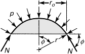
This result is valid anywhere in the shell, because N is observed not to vary with φ. Note that, in contrast with the case of plates, it is the midsurface that sustains the applied load.
Once again referring to the simple shell shown in Fig. 13.11, we demonstrate that the bending stresses play an insignificant role in the load-carrying mechanism. On the basis of the symmetry of the shell and the loading, the stresses (equal at any point) are given by
(a)
Here σn represents the compressive, in-plane stress. The stress normal to the mid-surface is negligible, and thus the in-plane strain involves only σn:
(b)
The reduced circumference associated with this strain is
2πr′ = 2π(r + rεn)
so
r′ = r(1 + εn)
The change in curvature is therefore
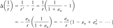
Dropping higher-order terms because of their negligible magnitude and substituting Eq. (b), this expression becomes
(c)
The bending moment in the shell is determined from the plate equations. Noting that 1/rx and 1/ry in Eq. (13.7) refer to the change in plate curvatures between the undeformed and deformed conditions, we see that for the spherical shell under consideration, Δ(1/r) = 1/rx = 1/ry. Therefore, Eq. (13.7) yields
(d)
and the maximum corresponding stress is
(e)
Comparing σb and σn [Eqs. (e) and (a)], we have
(13.45)
demonstrating that the in-plane or direct stress is very much larger than the bending stress, inasmuch as t/2r ≪ 1. It may be concluded, therefore, that the applied load is resisted primarily by the in-plane stressing of the shell.
Although the preceding discussion relates to the simplest shell configuration, the conclusions drawn with respect to the fundamental mechanism apply to any shape and loading at locations away from the boundaries or points of concentrated load application. If there are asymmetries in load or geometry, shearing stresses will exist in addition to the normal and bending stresses.
In the following sections we discuss the membrane theory of two common structures: the shell of revolution and cylindrical shells.
13.13 Symmetrically Loaded Shells of Revolution
A surface of revolution, such as in Fig. 13.12a, is formed by the rotation of a meridian curve (eo′) about the OO axis. As shown, a point on the shell is located by coordinates θ, φ, r0. This figure indicates that the elemental surface abcd is defined by two meridian and two parallel circles. The planes containing the principal radii of curvature at any point on the surface of the shell are the meridian plane and a plane perpendicular to it at the point in question. The meridian plane will thus contain rθ, which is related to side ab. The other principal radius of curvature, rφ, is found in the perpendicular plane and is therefore related to side bd. Thus, length ab = (rθ sin θ)dθ = r0 dθ, and length bd = rφ dφ.
Figure 13.12. Diagrams for analysis of symmetrically loaded shells of revolution: (a) geometry of the shell; (b) membrane forces (per unit length) and distributed loading (per unit area) acting on a shell element; (c) meridian forces and resultant of the loading acting on a truncated shell.
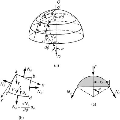
The condition of symmetry prescribes that no shearing forces act on the element and that the normal forces Nθ and Nφ per unit length display no variation with θ (Fig. 13.12b). These membrane forces are also referred to as the tangential or hoop and meridian forces, respectively. The name arises from the fact that forces of this kind exist in true membranes, such as soap films or thin sheets of rubber. The externally applied load is represented by the perpendicular components py and pz. We turn now to a derivation of the equations governing the force equilibrium of the element.
Equations of Equilibrium
To describe equilibrium in the z direction, it is necessary to consider the z components of the external loading as well as of the forces acting on each edge of the element. The external z-directed load acting on an element of area (r0 dθ)(rφdφ) is
(a)
The force acting on the top edge of the element is Nφ r0 dθ. Neglecting terms of higher order, the force acting on the bottom edge is also Nφ r0 dθ. The z component at each edge is then Nφ r0 dθ sin(dφ/2), which may be approximated by Nφ r0 dθ dφ/2, leading to a resultant for both edges of
(b)
The force on each side of the element is Nθrφ dφ. The radial resultant for both such forces is (Nθ rφ dφ)dθ, having a z-directed component
(c)
Adding the z forces, equating to zero, and canceling dθ dφ, we obtain
Nφr0 + Nθrφ sin φ + pzr0rφ = 0
Dividing by r0rφ and replacing r0 by rθ sin φ, this expression is converted to the following form:
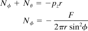
(13.46a)
Similarly, an equation for the y equilibrium of the element of the shell may also be derived. But instead of solving the z and y equilibrium equations simultaneously, it is more convenient to obtain Nφ from the equilibrium of the portion of the shell corresponding to the angle φ (Fig. 13.12c):
(13.46b)
Then calculate Nθ from Eq. (13.46a). Here F represents the resultant of all external loading acting on the portion of the shell.
Conditions of Compatibility
For the axisymmetrical shells considered, owing to their freedom of motion in the z direction, strains are produced such as to assure consistency with the field of stress. These strains are compatible with one another. It is clear that, when a shell is subjected to concentrated surface loadings or is constrained at its boundaries, membrane theory cannot satisfy the conditions on deformation everywhere. In such cases, however, the departure from membrane behavior is limited to a narrow zone in the vicinity of the boundary or the loading. Membrane theory remains valid for the major portion of the shell, but the complete solution can be obtained only through application of bending theory.
13.14 Some Common Cases of Shells of Revolution
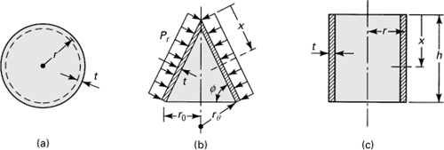
The membrane stresses in any particular axisymmetrically loaded shell in the form of a surface of revolution may be obtained readily from Eqs. (13.46). Treated next are three common structural members. It is interesting to note that, for the circular cylinder and the cone, the meridian is a straight line.
Spherical Shell (Fig. 13.13a)
We need only set the mean radius r = rθ = rφ and hence r0 = r sin φ. Equations (13.46) then become
(13.47)
Figure 13.13. Typical shells of revolution: (a) spherical shells; (b) conical shell under uniform pressure; (c) cylindrical shell.
Example 13.6 illustrates an application of this equation.
The simplest case is that of a spherical shell subjected to internal pressure p. We now have p = –pz, φ = 90°, and F = –πr2p. As is evident from the symmetry of a spherical shell, Nφ = Nθ = N. These quantities, introduced into Eqs. (13.47), lead to the membrane stress in a spherical pressure vessel:
(13.48)
where t is the thickness of the shell. Clearly, this equation represents uniform stresses in all directions of a pressurized sphere.
Conical Shell (Fig. 13.13b)
We need only set rφ = ∞ in Eq. (13.46a). This, together with Eq. (13.46b), provides the following pair of equations for determining the membrane forces under uniformly distributed load pz = pr:
(13.49)
Here x represents the direction of the generator. The hoop and meridian stresses in a conical shell are found by dividing Nθ and Nx by t, wherein t is the thickness of the shell.
Circular Cylindrical Shell (Fig. 13.13c)
To determine the membrane forces in a circular cylindrical shell, we begin with the cone equations, setting φ = π/2, pz = pr, and mean radius r = r0 = constant. Equations (13.49) are therefore
(13.50)
Here x represents the axial direction of the cylinder.
For a closed-ended cylindrical vessel under internal pressure, p = –pr and F = –πr2p. The preceding equations then result in the membrane stresses:
(13.51)
Here t is the thickness of the shell. Because of its direction, σθ is called the tangential, circumferential, or hoop stress; similarly, σx is the axial or the longitudinal stress. Note that for thin-walled cylindrical pressure vessels, σθ = 2σx. From Hooke’s law, the radial extension θ of the cylinder, under the action of tangential and axial stresses σθ and σx, is
(13.52)
where E and ν represent modulus of elasticity and Poisson’s ratio.
Observe that tangential stresses in the sphere are half the magnitude of the tangential stresses in the cylinder. Thus, a sphere is an optimum shape for an internally pressurized closed vessel.
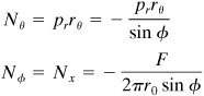
Example 13.5. Compressed Air Tank
A steel cylindrical vessel with hemispherical ends or so-called heads, supported by two cradles (Fig. 13.14), contains air at a pressure of p. Calculate (a) the stresses in the tank if each portion has the same mean radius r and the thickness t; (b) radial extension of the cylinder. Given: r = 0.5 m, t = 10 mm, p = 1.5 MPa, E = 200 GPa, and ν = 0.3. Assumptions: One of the cradles is designed so that it does not exert any axial force on the vessel; the cradles act as simple supports. The weight of the tank may be disregarded.
Figure 13.14. Example 13.5. Cylindrical vessel with spherical ends.
Solution
a. The axial stress in the cylinder and the tangential stresses in the spherical heads are the same.
Referring to Eqs. (13.51), we write
![]()
The tangential stress in the cylinder is therefore
![]()
b. Through the use of Eq. (13.52), we have
![]()
Comment
The largest radial stress, occurring on the surface of the tank, σr = p, is negligibly small compared with the tangential and axial stresses. The state of stress in the wall of a thin-walled vessel is thus taken to be biaxial.
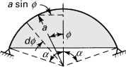
Example 13.6. Hemispherical Dome
Derive expressions for the stress resultants in a hemispherical dome of radius a and thickness t, loaded only by its own weight, p per unit area (Fig. 13.15).
Figure 13.15. Example 13.6. Simply supported hemispherical dome carries its own weight.
Solution
The weight of that portion of the dome intercepted by φ is
![]()
In addition,
pz = p cos φ
Substituting into Eqs. (13.46) for pz and F, we obtain
(13.53)
where the negative signs indicate compression. It is clear that Nφ is always compressive. The sign of Nθ, on the other hand, depends on φ. From the second expression, when Nθ = 0, φ = 51°50′. For φ smaller than this value, Nθ is compressive. For φ > 51°50′, Nθ is tensile.
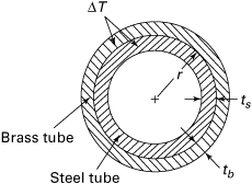
13.15 Thermal Stresses in Compound Cylinders
This section provides the basis for design of composite or compound multishell cylinders, constructed of a number of concentric, thin-walled shells. In the development that follows, each component shell is assumed homogeneous and isotropic. Each may have a different thickness and different material properties and be subjected to different uniform or variable temperature differentials [Refs. 13.7 and 13.8].
In the case of a free-edged multishell cylinder undergoing a uniform temperature change ΔT, the free motion of any shell having different material properties is restricted by components adjacent to it. Only a tangential or hoop stress σθ and corresponding strain εθ are then produced in the cylinder walls. Through the use of Eqs. (3.26a), with σy = σθ, εy = εθ, and T = ΔT, we write
(13.54)
where α is the coefficient of thermal expansion. In a cylinder subjected to a temperature gradient, both axial and hoop stresses occur, and σx = σθ = σ. Hence, Eq. (3.26b) leads to
(13.55)
Let us consider a compound cylinder consisting of three components, each under different temperature gradients (the ΔTs), as depicted in Fig. 13.16. Applying Eq. (13.55), the stresses may be expressed in the following form:
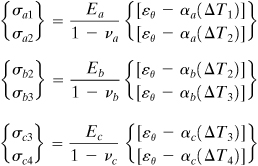
(13.56a-f)
Figure 13.16. Compound cylinder under a uniform temperature change.
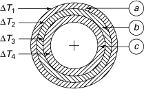
Here the subscripts a, b, and c refer to individual shells.
The axial forces corresponding to each layer are next determined from the stresses given by Eqs. (13.56) as
![]()
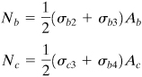
in which the A’s are the cross-sectional area of each component. The condition that the sum of the axial forces be equal to zero is satisfied when
(b)
Equations (13.56) together with Eqs. (a) and (b), for the case in which νa = νb = νc, lead to the following expression for the tangential strain:
(13.57)
Here the quantities (ΔT)a, (ΔT)b, and (ΔT)c represent the average of the temperature differentials at the boundaries of elements a, b, and c, respectively, for instance, ![]() . The stresses at the inner and outer surfaces of each shell may be obtained readily on carrying Eq. (13.57) into Eqs. (13.56).
. The stresses at the inner and outer surfaces of each shell may be obtained readily on carrying Eq. (13.57) into Eqs. (13.56).
A final point to be noted is that near the ends there will often be some bending of the composite cylinder, and the total thermal stresses will be obtained by superimposing on Eqs. (13.56) such stresses as may be necessary to satisfy the boundary conditions [Ref. 13.1].
Example 13.7. Brass-Steel Cylinder
The cylindrical part of a jet nozzle is made by just slipping a steel tube over a brass tube with each shell uniformly heated and the temperature raised by ΔT (Figure 13.17). Determine the hoop stress that develops in each component on cooling. Assumptions: Coefficient of thermal expansion of the brass is larger than that of steel (see Table D.1). Each tube is a thin-walled shell with a mean radius of r.
Figure 13.17. Example 13.7. Two-layer compound cylinder.
Solution
For the condition described, the composite cylinder is contracting. Equation (13.54) is therefore
(13.58)
from which
(13.59)
We have Ab = 2πrtb and As = 2πrts, in which tb and ts represent the wall thickness of the brass and steel tubes, respectively. Hoop strain, referring to Eqs. (13.57) and (13.59), is written as
(13.60)
Finally, hoop stresses, through the use of Eqs. (13.58) and (13.60) and after simplification, are determined as follows:
(13.61)
(13.62)
Comment
Observe that the stresses in the brass and steel tubes are tensile and compressive, respectively, since αb > αs, and ΔT is a negative quantity because of cooling.
13.16 Cylindrical Shells of General Shape
A cylindrical shell generated as a straight line, the generator, moves parallel to itself along a closed path. Figure 13.18 shows an element isolated from a cylindrical shell of arbitrary cross section. The element is located by coordinates x (axial) and θ on the cylindrical surface.
Figure 13.18. Membrane forces (per unit length) and distributed axial, radial, and tangential loads (per unit area) on a cylindrical shell element.
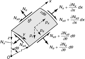
The forces acting on the sides of the element are depicted in the figure. The x and θ components of the externally applied forces per unit area are denoted px and pθ and are shown to act in the directions of increasing x and θ (or y). In addition, a radial (or normal) component of the external loading pr acts in the positive z direction. The following expressions describe the requirements for equilibrium in the x, θ, and r directions:
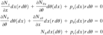
Canceling the differential quantities, we obtain the equations of a cylindrical shell:
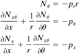
(13.63)
Given the external loading, Nθ is readily determined from the first equation of (13.63). Following this, by integrating the second and the third equations, Nxθ and Nx are found:
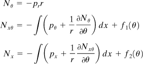
(13.64)
Here f1(θ) and f2(θ) represent arbitrary functions of integration to be evaluated on the basis of the boundary conditions. They arise, of course, as a result of the integration of partial derivatives.
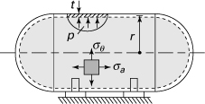
Example 13.8. Liquid Tank
Determine the stress resultants in a circular, simply supported tube of thickness t filled to capacity with a liquid of specific weight γ (Fig. 13.19a).
Figure 13.19. Example 13.8. Cylindrical tube filled with liquid.
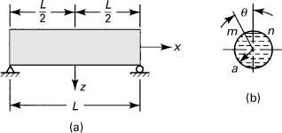
Solution
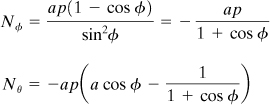
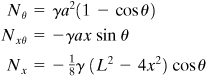
The pressure at any point in the tube equals the weight of a column of unit cross-sectional area of the liquid at that point. At the arbitrary level mn (Fig. 13.19b), the outward pressure is –γa(1 – cos θ), where the pressure is positive radially inward; hence the minus sign. Then
(a)
Substituting the foregoing into Eqs. (13.64), we obtain
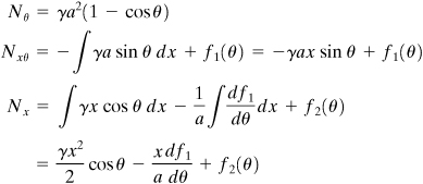
(b)
The boundary conditions are
(c)
The introduction of Eq. (b) into Eq. (c) leads to
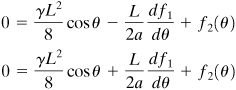
Addition and subtraction of these give, respectively,
(d)
We observe from the second equation of (b) that c in the second equation of (d) represents the value of the uniform shear load Nxθ at x = 0. This load is zero because the tube is subjected to no torque; thus c = 0. Then, Eq. (b), together with Eq. (d), provides the solution:
(13-65)
The stresses are determined upon dividing these stress resultants by the shell thickness. It is observed that the shear Nxθ and the normal force Nx exhibit the same spanwise distribution as do the shear force and the bending moment of a beam. Their values, as may be readily verified, are identical with those obtained by application of the beam formulas, Eqs. (5.39) and (5.38), respectively.
It has been noted that membrane theory cannot, in all cases, provide solutions compatible with the actual conditions of deformation. This theory also fails to predict the state of stress in certain areas of the shell. To overcome these shortcomings, bending theory is applied in the case of cylindrical shells, taking into account the stress resultants such as the types shown in Fig. 13.3 and Nx, Nθ, and Nxθ.
References
13.1. UGURAL, A. C., Stresses in Beams, Plates, and Shells, 3rd ed., CRC Press, Taylor and Francis Group, Boca Raton, Fla., 2010.
13.2. TIMOSHENKO, S. P., and WOINOWSKY-KRIEGER, S., Theory of Plates and Shells, 2nd ed., McGraw-Hill, New York, 1959.
13.3. YANG, T. Y., Finite Element Structural Analysis, Prentice Hall, Upper Saddle River, N.J., 1986.
13.4. BATHE, K. I., Finite Element Procedures in Engineering Analysis, Prentice Hall, Upper Saddle River, N.J., 1996.
13.5. ZIENKIEWICZ, O. C., and TAYLOR, R. I., The Finite Element Method, 4th ed., Vol. 2 (Solid and Fluid Mechanics, Dynamics and Nonlinearity), McGraw-Hill, London, 1991.
13.6. BAKER, A. J., and PEPPER, D. W., Finite Elements 1=2=3, McGraw-Hill, New York, 1991.
13.7. ABRAHAM, L. H., Structural Design of Missiles and Spacecraft, McGraw-Hill, New York, 1963.
13.8. FAUPEL, J. H., and FISHER, F. E., Engineering Design, 2nd ed., Wiley, Hoboken, N. J., 1981.
Problems
Sections 13.1 through 13.10
13.1. A uniform load po acts on a long and narrow rectangular plate with edges at y = 0 and y = b both clamped (Fig. 13.6). Determine (a) the equation of the surface deflection and (b) the maximum stress σy at the clamped edge. Use ![]() .
.
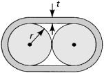
13.2. An initially straight steel band 30-mm wide and t = 0.3-mm thick is used to lash together two drums of radii r = 120 mm (Fig. P13.2). Using E = 200 GPa and ν = 0.3, calculate the maximum bending strain and maximum stress developed in the band.
13.3. For the plate described in Example 13.1, for po = 20 kN/m2, b = 0.6 m, t = 12 mm, E = 200 GPa, and ![]() , calculate the maximum deflection wmax, maximum strain εy, max, maximum stress σy, max, and the radius of the midsurface.
, calculate the maximum deflection wmax, maximum strain εy, max, maximum stress σy, max, and the radius of the midsurface.
13.4. A thin rectangular plate is subjected to uniformly distributed bending moments Ma and Mb applied along edges a and b, respectively. Derive the equations governing the surface deflection for two cases: (a) Ma ≠ Mb and (b) Ma = –Mb.
13.5. The simply supported rectangular plate shown in Fig. 13.7a is subjected to a distributed load p given by
![]()
Derive an expression for the deflection of the plate in terms of the constants P, a, b, and D.
13.6. A simply supported square plate (a = b) carries the loading
![]()
(a) Determine the maximum deflection. (b) Retaining the first two terms of the series solutions, evaluate the value of po for which the maximum deflection is not to exceed 8 mm. The following data apply: a = 3 m, t = 25 mm, E = 210 GPa, and ν = 0.3.
13.7. A clamped circular plate of radius a and thickness t is to close a circuit by deflecting 1.5 mm at the center at a pressure of p = 10 MPa. (Fig. 13.9). What is the required value of t? Take a = 50 mm, E = 200 GPa, and ν = 0.3.
13.8. A simply supported circular plate of radius a and thickness t is deformed by a moment Mo uniformly distributed along the edge. Derive an expression for the deflection w as well as for the maximum radial and tangential stresses.
13.9. Given a simply supported circular plate containing a circular hole (r = b), supported at its outer edge (r = a) and subjected to uniformly distributed inner edge moments Mo, derive an expression for the plate deflection.
13.10. A brass flat clamped disk valve of 0.4-m diameter and 20-mm thickness is subjected to a liquid pressure of 400 kPa (Fig. 13.9). Determine the factor of safety, assuming that failure occurs in accordance with the maximum shear stress theory. The yield strength of the material is 100 MPa and ![]() .
.
13.11. A circular plate of radius a is simply supported at its edge and subjected to uniform loading po. Determine the center point deflection.
13.12. A rectangular aluminum alloy sheet of 6-mm thickness is bent into a circular cylinder with radius r. Calculate the diameter of the cylinder and the maximum moment developed in the member if the allowable stress is not to exceed 120 MPa, E = 70 GPa, and ν = 0.3.
13.13. The uniform load p0 acts on a long and narrow rectangular plate with edge y = 0 simply supported and edge y = b clamped, as depicted in Figure P13.13. Find (a) the equation of the surface deflection w; (b) the maximum bending stress.
13.14. An approximate expression for the deflection surface of a clamped triangular plate (Figure P13.14) is given as follows:
(P13.14)
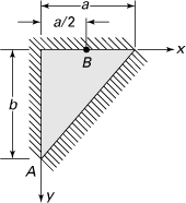
in which c is a constant. (a) Show that Equation P13.14 satisfies the boundary conditions. (b) Find the approximate maximum plane stress components at points A and B.
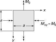
13.15. A square instrument panel (Figure P13.15) is under uniformly distributed twisting moment Mxy = M0 at all four edges. Find an expression for the deflection surface w.
13.16. A cylindrical thick-walled vessel of 0.2-m radius and flat, thin plate head is subjected to all internal pressure of 1.5 MPa. Calculate (a) the thickness of the cylinder head if the allowable stress is limited to 135 MPa; (b) the maximum deflection of the cylinder head. Given: E = 200 GPa and ν = 0.3.
13.17. A high-strength, ASTM-A242 steel plate covers a circular opening of diameter d = 2a. Assumptions: The plate is fixed at its edge and carries a uniform pressure po. Given: E = 200 GPa, σyp = 345 MPa (Table D.1), v = 0.3, t = 10 mm, a = 125 mm. Calculate (a) the pressure po, and maximum deflection at the onset of yield in the plate; (b) allowable pressure based on a safety factor of n = 1.2 with respect to yielding of the plate.
13.18. A 500-mm simply supported square aluminum panel of 20-mm thickness is under uniform pressure po. For E = 70 GPa, ν = 0.3, and σyp = 240 MPa and taking into account only the first term of the series solution, calculate the limiting value of po that can be applied to the plate without causing yielding and the maximum deflection w that would be produced when po reaches its limiting value.
13.19. Verify that integrating Eq. (b) of Section 13.9 results in Eq. (c).
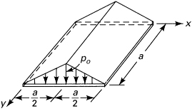
13.20. Apply the Rayleigh–Ritz method to determine the maximum deflection of a simply supported square plate subjected to a lateral load in the form of a triangular prism (Fig. P13.20).
Sections 13.11 through 13.16
13.21. Consider two pressurized vessels of cylindrical and spherical shapes of mean radius r = 150 mm (Figure 13.13), constructed of 6-mm-thick plastic material. Find the limiting value of the pressure differential the shells can resist given a maximum stress of 15 MPa.
13.22. A spherical vessel of radius r = 1 m and wall thickness t = 50 mm is submerged in water having density γ = 9.81 kN/m3. On the basis of a factor of safety of n = 2, calculate the water depth at which the tangential stress σθ in the sphere would be 30 MPa.
13.23. Figure P13.23 shows a closed-ended cylindrical steel tank of a radius r = 4 m and a height h = 18 m. The vessel is completely filled with a liquid of density γ = 15 kN/m3 and is subjected to an additional internal gas pressure of p = 500 kPa. Based on an allowable stress of 180 MPa, calculate the wall thickness needed (a) at the top of the tank; (b) at quarter-height of the tank; (c) at the bottom of the tank.
13.24. Resolve Prob. 13.23, assuming that the gas pressure is p = 200 kPa.
13.25. A cylinder of 1.2 m in diameter, made of steel with maximum strength σmax = 240 MPa, is under an internal pressure of p = 1.2 kPa. Calculate the required thickness t of the vessel on the basis of a factor of safety n = 2.4.
13.26. A pipe for conveying water (density γ = 9.81 kN/m3) to a turbine, called penstock, operates at a head of 150 m. The pipe has a 0.8-m diameter and a wall thickness of t. Find the minimum required value of t for a material strength of 120 MPa based on a safety factor of n = 1.8.
13.27. Resolve Prob. 13.26 if the allowable stress is 100 MPa.
13.28. A closed cylindrical tank fabricated of 12-mm-thick plate is under an internal pressure of p = 10 MPa. Calculate (a) the maximum diameter if the maximum shear stress is limited to 35 MPa; (b) the limiting value of tensile stress for the diameter found in part (a).
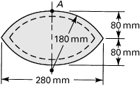
13.29. Given an internal pressure of 80 kPa, calculate the maximum stress at point A of a football of uniform skin thickness t = 2 mm (Fig. P13.29).
13.30. For the toroidal shell of Fig. P13.30 subjected to internal pressure p, determine the membrane forces Nφ and Nθ.
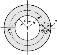
13.31. A toroidal pressure vessel of outer and inner diameters 1 and 0.7 m, respectively, is to be used to store air at a pressure of 2 MPa. Determine the required minimum thickness of the vessel if the allowable stress is not to exceed 210 MPa.
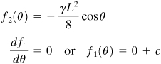
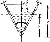
13.32. Show that the tangential (circumferential) and longitudinal stresses in a simply supported conical tank filled with liquid of specific weight γ (Fig. P13.32) are given by
(13.32)
13.33. A simply supported circular cylindrical shell of radius a and length L carries its own weight p per unit area (that is, px = 0, pθ = –p cos θ, and pr = p sin θ). Determine the membrane forces. The angle θ is measured from the horizontal axis.
13.34. Redo Example 13.8 for the case in which the ends of the cylinder are fixed.
13.35. An edge-supported conical shell carries its own weight p per unit area and is subjected to an external pressure pr (Fig. 13.13b). Determine the membrane forces and the maximum stresses in the shell.