Appendix C. Moments of Composite Areas
C.1 Centroid
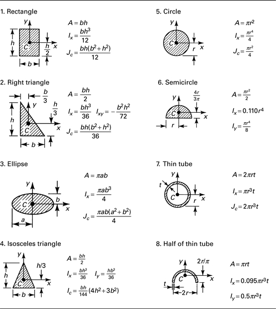
This appendix is concerned with the geometric properties of cross sections of a member. These plane area characteristics have special significance in various relationships governing stress and deflection of beams, columns, and shafts. Geometric properties for most areas encountered in practice are listed in numerous reference works [Ref. C.1]. Table C.1 presents several typical cases.
Table C.1. Properties of Some Plane Areas
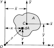
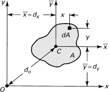
The first step in evaluating the characteristics of a plane area is to locate the centroid of the area. The centroid is the point in the plane about which the area is equally distributed. For area A shown in Fig. C.1, the first moments about the x and y axes, respectively, are given by
(C.1)
Figure C.1. Plane area A with centroid C.
These properties are expressed in cubic meters or cubic millimeters in SI units and in cubic feet or cubic inches in U.S. Customary Units. The centroid of area A is denoted by point C, whose coordinates ![]() and
and ![]() satisfy the relations
satisfy the relations
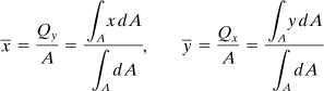
(C.2)
When an axis possesses an axis of symmetry, the centroid is located on that axis, as the first moment about an axis of symmetry equals zero. When there are two axes of symmetry, the centroid lies at the intersection of the two axes. If an area possesses no axes of symmetry but does have a center of symmetry, the centroid coincides with the center of symmetry.
Example C.1. Centroid of Triangular Area
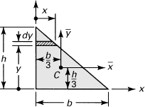
Determine the ordinate ![]() of the centroid of the triangular area shown in Fig. C.2.
of the centroid of the triangular area shown in Fig. C.2.
Figure C.2. Example C.1. Triangular area.
Solution
A horizontal element with area of length x and height dy is selected (Fig. C.2). Considering similar triangles, x = (h – y)b/h, and
![]()
The first moment of the area with respect to the x axis is
![]()
The second of Eqs. (C.2), with A = bh/2, then yields
(a)
Therefore, the centroidal axis ![]() of the triangular area is located a distance of one-third the altitude from the base of the triangle.
of the triangular area is located a distance of one-third the altitude from the base of the triangle.
Similarly, choosing the element of area dA as a vertical strip, it can be shown that the abscissa of the centroid is ![]() = b/3. The location of the centroid C is shown in the figure.
= b/3. The location of the centroid C is shown in the figure.
Frequently, an area can be divided into simple geometric shapes (for example, rectangles, circles, and triangles) whose areas and centroidal coordinates are known or easily determined. When a composite area is considered as an assemblage of n elementary shapes, the resultant or total area is the algebraic sum of the separate areas, and the resultant moment about any axis is the algebraic sum of the moments of the component areas. Thus, the centroid of a composite area has the coordinates
(C.3)
in which ![]() and
and ![]() represent the coordinates of the centroids of the component areas Ai(i = 1, 2, ..., n).
represent the coordinates of the centroids of the component areas Ai(i = 1, 2, ..., n).
In applying formulas (C.3), it is important to sketch the simple geometric forms into which the composite area is resolved, as shown next.
Example C.2. Centroid of an Angle
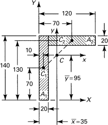
Locate the centroid of the angle section depicted in Fig. C.3. The dimensions are given in millimeters.
Figure C.3. Example C.2. Area consisting of two parts.
Solution
The composite area is divided into two rectangles, A1 and A2, for which the centroids are known (Fig. C.3). Taking the X,Y axes as reference, Eqs. (C.3) are applied to calculate the coordinates of the centroid. The computation is conveniently carried out in the following tabular form. Note that when an area is divided into only two parts, the centroid C of the entire area always lies on the line connecting the centroids C1 and C2 of the components, as indicated in Fig. C.3.
C.2 Moments of Inertia
We now consider the second moment or moment of inertia of an area (a relative measure of the manner in which the area is distributed about any axis of interest). The moments of inertia of a plane area A with respect to the x and y axes, respectively, are defined by the following integrals:
(C.4)
where x and y are the coordinates of the element of area dA (Fig. C.1).
Similarly, the polar moment of inertia of a plane area A with respect to an axis through O perpendicular to the area is given by
(C.5)
Here ρ is the distance from point O to the element dA, and ρ2 = x2 + y2. The product of inertia of a plane area A with respect to the x and y axes is defined as
(C.6)
In the foregoing, each element of area dA is multiplied by the product of its coordinates (Fig. C.1). The product of inertia of an area about any pair of axes is zero when either of the axes is an axis of symmetry.
From Eqs. (C.4) and (C.5), it is clear that the moments of inertia are always positive quantities because coordinates x and y are squared. Their dimensions are length raised to the fourth power; typical units are meters4, millimeters4, and inches4. The dimensions of the product of inertia are the same as for the moments of inertia; however, the product of inertia can be positive, negative, or zero depending on the values of the product xy.
The radius of gyration is a distance from a reference axis or a point at which the entire area of a section may be considered to be concentrated and still possess the same moment of inertia as the original area. Therefore, the radii of gyration of an area A about the x and y axes and the origin O (Fig. C.1) are defined as the quantities rx, ry, and ro, respectively:
(C.7)
Substituting Ix, Iy, and Jo from Eqs. (C.7) into Eq. (C.5) results in
(C.8)
The radius of gyration has the dimension of length, expressed in meters.
C.3 Parallel-Axis Theorem
The moment of inertia of an area with respect to any axis is related to the moment of inertia around a parallel axis through the centroid by the parallel-axis theorem, sometimes called the transfer formula. It is useful for determining the moment of inertia of an area composed of several simple shapes.
To develop the parallel-axis theorem, consider the area A depicted in Fig. C.4. Let ![]() and
and ![]() represent the centroidal axes of the area, parallel to the axes x and y, respectively. The distances between the two sets of axes and the origin are dx, dy, and do. The moment of inertia with respect to the x axis is
represent the centroidal axes of the area, parallel to the axes x and y, respectively. The distances between the two sets of axes and the origin are dx, dy, and do. The moment of inertia with respect to the x axis is
![]()
Figure C.4. Plane area for deriving the parallel-axis theorem.
The first integral on the right side equals the moment of inertia ![]() about the
about the ![]() axis. As y is measured from the centroid axis
axis. As y is measured from the centroid axis ![]() , ∫Ay dA is zero. Hence,
, ∫Ay dA is zero. Hence,
(C.9a)
Similarly,
(C.9b)
The parallel-axis theorem is thus stated as follows: The moment of inertia of an area with respect to any axis is equal to the moment of inertia around a parallel centroidal axis, plus the product of the area and the square of the distance between the two axes.
In a like manner, a relationship may be developed connecting the polar moment of inertia Jo of an area about an arbitrary point O and the polar moment of inertia Jc about the centroid of the area (Fig. C.4):
(C.10)
It can be shown that the product of inertia of an area Ixy with respect to any set of axes is given by the transfer formula
(C.11)
where ![]() denotes the product of inertia around the centroidal axes. Note that the parallel-axis theorems, Eqs. (C.9) through (C.11), may be employed only if one of the two axes involved is a centroidal axis.
denotes the product of inertia around the centroidal axes. Note that the parallel-axis theorems, Eqs. (C.9) through (C.11), may be employed only if one of the two axes involved is a centroidal axis.
For elementary shapes, the integrals appearing in the equations of this and preceding sections can usually be evaluated easily and the geometric properties of the area thus obtained (Table C.1). Cross-sectional areas employed in practice can often be broken into a combination of these simple shapes.
Example C.3. Moments of Inertia for a Triangular Area
For the triangular area shown in Fig. C.2, determine (a) the moment of inertia about the ![]() and x axes and (b) the products of inertia with respect to the
and x axes and (b) the products of inertia with respect to the ![]() and xy axes.
and xy axes.
Solution
The area of a horizontal strip selected is
(a)
and the coordinates are related by
(b)
as already found in Example C.1.
a. Then the moment of inertia about the centroidal ![]() axis is (Fig. C.2)
axis is (Fig. C.2)
(c)
Similarly, the moment of inertia with respect to the x axis equals
(d)
This solution may also be obtained by applying the parallel-axis theorem:
![]()
where dy = ![]() is the distance between the x and
is the distance between the x and ![]() axes.
axes.
b. From considerations of symmetry, the product of inertia of the horizontal strip with respect to the axes through its own centroid and parallel to the xy axes is zero. Its product of inertia about the xy axes, using Eq. (C.11), is then
![]()
Here ![]() and
and ![]() are the distances to the centroid of the strip. Referring to Fig. C.2, we have
are the distances to the centroid of the strip. Referring to Fig. C.2, we have ![]() and
and ![]() . Substituting these together with Eqs. (a) and (b) into the preceding equation, we have
. Substituting these together with Eqs. (a) and (b) into the preceding equation, we have
(e)
The transfer formula now yields the product of inertia with respect to the centroidal axes:
![]()
Example C.4. Moment of Inertia for a T Section
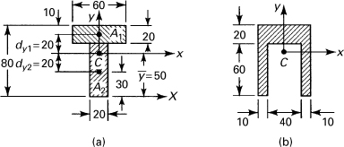
Determine the moment of inertia of the T section shown in Fig. C.5a around the horizontal axis passing through its centroid. The dimensions are given in millimeters.
Figure C.5. Example C.4. (a) T section; (b) channel section.
Solution
Location of centroid: The area is divided into component parts A1 and A2 for which the centroids are known (Fig. C.5a). Because the y axis is an axis of symmetry, ![]() , and
, and
![]()
Centroidal moment of inertia: Application of the transfer formula to Fig. C.5a results in
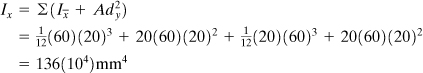
Interestingly, the properties of this T section about the centroidal x axis are the same as those of the channel (Fig. C.5b). Both sections possess an axis of symmetry.
C.4 Principal Moments of Inertia
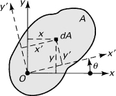
The moments of inertia of a plane area depend not only on the location of the reference axis but also on the orientation of the axes about the origin. The variation of these properties with respect to axis location are governed by the parallel-axis theorem, as described in Section C.3. We now derive the equations for transformation of the moments and product of inertia at any point of a plane area.
The area shown in Fig C.6 has the moments and product of inertia Ix, Iy, Ixy with respect to the x and y axes defined by Eqs. (C.4) and (C.6). It is required to determine the moments and product of inertia Ix′, Iy′, and Ix′y′ about axes x′, y′ making an angle θ with the original x, y axes. The new coordinates of an element dA can be expressed by projecting x and y onto the rotated axes (Fig. C.6):
(a)
Then, by definition
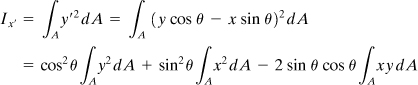
Upon substituting Eqs. (C.4) and (C.6), the foregoing becomes
(b)
The moment of inertia Iy′ may be found readily by substituting θ + π/2 for θ in the expression for Ix′. Similarly, using the definition Ix′y′ = ∫Ax′y′dA, we obtain
(c)
The transformation equations for the moments and product of inertia may be rewritten by introducing double-angle trigonometric relations in the form
(C.12a)
(C.12b)
(C.12c)
In comparing the expressions here and in Chapter 1, it is observed that moments of inertia (Ix, Iy, Ix′, Iy′) correspond to the normal stresses (σx, σy, σx′, σy′) the negative of the products of inertia (–Ixy, –Ix′y′) correspond to the shear stresses (τxy, τx′y′), and the polar moment of inertia (Jo) corresponds to the sum of the normal stresses (σx + σy). Thus, Mohr’s circle analysis and the characteristics for stress apply to these properties of area.
The angle θ at which the moment of inertia Ix′ of Eq. (C.12a) assumes an extreme value may be obtained from the condition dIx′/dθ = 0:
(d)
The foregoing yields
(C.13)
Here θp represents the two values of θ that locate the principal axes about which the principal or maximum and minimum moments of inertia occur.
When Eq. (C.12c) is compared with Eq. (d), it becomes clear that the product of inertia is zero for the principal axes. If the origin of axes is located at the centroid of the area, they are referred to as the centroidal principal axes. It was observed in Section 3.2 that the products of inertia relative to the axes of symmetry are zero. Thus, an axis of symmetry coincides with a centroidal principal axis.
The principal moments of inertia are determined by introducing the two values of θp into Eq. (C.12a). The sine and cosine of angles 2θp defined by Eq. (C.13) are
(e)
where ![]() . When these expressions are inserted into Eq. (C.12a), we obtain
. When these expressions are inserted into Eq. (C.12a), we obtain
(C.14)
wherein I1 and I2 denote the maximum and minimum principal moments of inertia, respectively.
Example C.5. Principal Moments of Inertia for Angular Section
Calculate the centroidal principal moments of inertia for the angular section shown in Fig. C.7a. The dimensions are given in millimeters.
Figure C.7. Example C.5. (a) Angle section; (b) Mohr’s circle for moments of inertia.
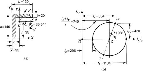
Solution
Location of centroid: The x, y axes are the reference axes through the centroid C (Fig. C.7a), the location of which has already been determined in Example C.2. Again, the area is divided into rectangles A1 and A2.
Moments of inertia: Applying the parallel-axis theorem, with reference to the x and y axes, we have
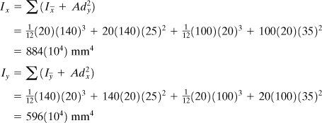
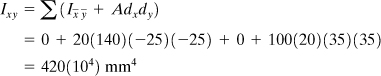
The product of inertia about the xy axes is obtained as described in Section C.3:
Principal moments of inertia: Equation (C.13) yields
![]()
Thus, the two values of θp are –35.54° and –125.54°. Using the first of these values, Eq. (C.12a) results in Ix′ = 1184(104) mm4. The principal moments of inertia are, from Eq. (C.14),
![]()
or I1 = Ix′ = 1184(104) mm4 and I2 = Iy′ = 296(104) mm4. The principal axes are indicated in Fig. C.7a as the x′y′ axes.
The principal moments of inertia may also be determined readily by means of Mohr’s circle, following a procedure similar to that described in Section 1.10, as shown in Fig. C.7b. Note that the quantities indicated are expressed in cm4 and the results are obtained analytically from the geometry of the circle.
Example C.6. General Formulation of Moments of Inertia for Angle Section
Derive general expressions for the centroidal moments and product of inertia for the angle section shown in Fig. C.7a. Write a computer program for the centroidal principal moments of inertia.
Solution
Using the X, Y axes as reference (Fig. C.7a), Eqs. (C.3) yield
(f)
(g)
The transfer formula (C.9a) results in
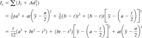
(h)
Similarly,
(i)
(j)
For convenience in programming, we employ the notation
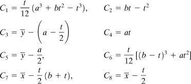
and
![]()
Equations (h), (i), (j), (C.13), and (C.14) are thus
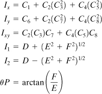
The required computer program, written in FORTRAN, is presented in Table C.2, along with input data (from Example C.5) and output values. The program was written and tested on a digital computer.
Table C.2. FORTRAN Program for Moments of Inertia
Reference
C.1. YOUNG, W. C., Roark’s Formulas for Stress and Strain, 6th ed., McGraw-Hill, New York, 1989, Chap. 5.