Chapter 19

Objective Measurement and Subjective Evaluations

The history of audio has had a frustrating tendency to produce ‘undefinables’ in terms of quality differences. The hi-fi press has invented a whole vocabulary of adjectives to describe sound qualities, but without objective verification there is no way to know if the terms mean the same thing to different people, or not. Spaciousness is one obvious example. In the stereo reproduction of music, spaciousness is a highly valued attribute, yet no unit of measurement exists for its quantification. Transparency is another example: we think that we know when we hear it, but can we prove it?

19.1 Objective Testing

In 1998, Dr Keith Holland began a series of loudspeaker tests, carried out at the Institute of Sound and Vibration Research (ISVR), for the magazine Studio Sound. His format can be followed here in order to present a series of objective measurements in a logical form. In a summary article, after about 20 tests had been performed on small loudspeakers, all intended for close-field or mid-field studio monitoring purposes, it was pointed out that no two responses of any aspect of the performance of any two of the loudspeakers was the same. People are often heard to ask why so many loudspeakers sound so different when they all measure the same. Well they may seem to measure the same when reading the manufacturers’ sanitised literature, but as Dr Holland pointed out, they do not sound the same simply because they do not measure the same.

Figures 19.1–19.4, 19.6, 19.9 and 19.10 show the anechoic responses of three different loudspeakers. In each case (except 19.3(c)) the (a) plot is that of a JBL LSR32, the (b) plot is that of a Westlake Audio BBSM-5 and the (c) plot is a Tannoy System 600A. The pedigree of the manufacturers is beyond reproach, yet they have chosen three radically different physical layouts. The JBL is a conventional vertical 3-way design, the Tannoy is a 2-way concentric design, and the Westlake is a 2-way design using horizontally spaced low frequency drivers with the tweeter mounted above and between them.

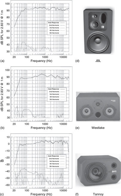
Figure 19.1 On-axis frequency response and harmonic distortion of three loudspeakers with physically very different driver layouts: (a) JBL LSR-32, (b) Westlake BBSM-5 and (c) Tannoy System 600A. (d) The JBL LSR-32, with 300 mm low frequency driver, (e) The Westlake BBSM-5, with 2 × 125 mm low frequency drivers and (f) The Tannoy System 600A, with 150 mm low frequency driver and coaxial tweeter

19.1.1 Pressure Amplitude Responses

Figure 19.1 shows the on-axis pressure amplitude responses and the distortion components up to the fifth harmonic. The axial frequency response was measured with the loudspeaker mounted on top of a pole in the large anechoic chamber at the ISVR. The microphone was a Bruel and Kjaer type 4133 mounted on a pole 1.7 m away from the loudspeaker. The measurement amplifier was a B & K 2609. The distance of 1.7 m was chosen in order to be distant enough to avoid geometrical and near-field effects, but close enough to achieve a good signal to noise ratio. Where relevant, the microphone was placed between the geometric centres of the low and high frequency drivers, although the true ‘acoustic centre’ of many loudspeakers is not well defined. Pink noise was used as the test signal to ensure a good signal to noise ratio throughout the audio bandwidth. The input signal was measured at the loudspeaker input terminals, thus eliminating power amplifier and loudspeaker cable effects, and the frequency response was derived from the output of the microphone pre-amplifier and the reference input signal.

Strictly speaking, the complete frequency response should show the pressure amplitude response and the phase response, but the phase responses have been omitted because of the notorious difficulty of interpreting them on the logarithmic scale that best suits the interpretation of the pressure amplitude plots. The phase plots have been replaced by ‘acoustic source’ plots, which will be described in sub-Section 19.1.4. The measurements were analysed with a 16,384-frequency line resolution, from 0Hz to 20 kHz, after averaging 160 records.

19.1.2 Harmonic Distortion

The harmonic distortion was measured by feeding the loudspeaker with a swept sine wave input. The sweep lasted for one minute, during which time it swept logarithmically from 10Hz to 10 kHz. The signal level was adjusted to give the equivalent level of 90dB SPL at one-metre distance. A test signal analysis was carried out to ensure that any harmonics it contained were below the noise floor. Only harmonics above −60dB (0.1%) are displayed.

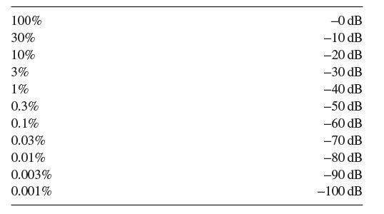
For reference, Table 19.1 shows a comparison of distortion figures in decibels and percentages.

Table 19.1 Equivalent harmonic distortion quantities

19.1.3 Directivity

The directivity plots show the horizontal and vertical off-axis responses. The measurement techniques were similar to those used for the axial pressure amplitude responses. The microphone position remained the same, but the loudspeakers were turned on the pole in increments of 15°.

19.1.4 Acoustic Source

As an alternative to the presentation of the phase responses, acoustic source plots are shown which were derived from the phase responses. The group delay was calculated as a phase slope (the differential of the phase response relative to frequency) and the results were derived from the multiplication of the group delay by the speed of sound. The acoustic source was plotted as an equivalent distance in metres that each frequency apparently emanated from in relation to the front baffle. It will be seen that the steeper the low frequency cut off, the further behind the front baffle will be the apparent acoustic source of the low frequencies.

19.1.5 Step-Function Response

The step response was calculated from the time integral of the inverse Fourier transform of the on-axis, high-resolution, complete frequency response (i.e. the pressure amplitude and phase responses). The step-function response shows the equivalent effect of the application of a DC voltage directly to the loudspeaker, and gives a good representation of the transient performance.

19.1.6 The Power Cepstrum

The power cepstrum is the Fourier transform of the logarithm of the pressure amplitude response. The resultant chart has units of time versus nondimensional decibels. Full details of the methodology can be found in the reference at the end of this chapter.¹ Cepstrum analysis evolved from the world of seismology, as a means of finding echo patterns in conditions of very poor signal-to-noise ratios. Some of the more or less equivalent terms are listed below, all of which are anagrams:

spectrum – cepstrum

frequency – quefrency

magnitude – gamnitude

phase – saphe

filter – lifter

harmonic – rahmonic

In this strange, pseudo-dimensional domain, ‘high-pass filters’ become ‘long pass lifters’.

Of particular value is the fact that reflexions and echoes show up very clearly as spikes in the power cepstra, even though these may not be apparent from the disturbances that they cause in the frequency response plots. Edge diffractions and diaphragm termination effects can be separated from the confusion of the general response. The displacement of a spike along the quefrency axis represents the delay in milliseconds separating the direct sound from the reflexion. The height of the spikes shows their relative strength. From the cepstrum display, one can readily compute the possible positions of the sources of the reflexions.

19.2 The On-Axis Pressure Amplitude Response

The on-axis pressure amplitude response is generally considered the most important of all loudspeaker specifications. For studio monitoring purposes it is widely accepted that this response should be as even and smooth as possible, although gradual roll-offs above 8 or 10 kHz are sometimes specified. Ideally, in many cases, relative uniformity of response down to 20Hz would be desirable, but this is only achieved in rare circumstances, partly because of the physical size necessary to generate 20Hz at realistic monitoring levels. It is therefore not considered a fault if smaller loudspeakers fail to reach down to 20Hz.

Although the frequency of roll-off and the rate of roll-off can have a great effect on the character of the low frequency sound, no consensus exists as to exactly where and how the roll-off should occur (i.e. the frequency and the slope). What is more, it is difficult to specify the necessary anechoic response of the loudspeakers because the rooms in which they are used, and the position within those rooms, not to mention whether the loudspeakers are mounted on meter bridges or on stands behind the mixing consoles, all seriously affect the in-room frequency response.

Looking at Figure 19.1 it can be seen that all three loudspeakers maintain a frequency response within ±4dB (from an arbitrary medium frequency) between 60Hz and about 19 kHz. The JBL maintains a response ±2.5dB from 70Hz to 20 kHz, which is quite remarkable for any loudspeaker. The low frequency roll-off is approximately third order (18dB per octave). The Tannoy maintains its frequency response to within ±4dB from 40Hz to 19 kHz, which is again a commendable performance, but the roll-off rates are very rapid at each end of the spectrum. At low frequencies, the roll-off is sixth order (36dB per octave [each ‘order’ representing 6dB per octave]). The Westlake also maintains ±4dB, this time between 40Hz and 20 kHz (and probably beyond) and exhibits a fourth order (24dB per octave) roll-off at low frequencies.

On closer inspection, the responses show definite differences of design approach. The JBL clearly tries to adhere to a flat response, and the low frequency roll-off is the most gradual of the three. The relatively large (300 mm) woofer and the 50 litre cabinet allow this with reasonable sensitivity (93dB at 1 m for 2.83 V). With these dimensions, the low frequencies do not need to be ‘forced’ by special tuning alignment or electrical boosts. The Tannoy [Figure 19.1 (c) and (f)] displays a very gradually falling low frequency response, but there is a general trend towards the response rising with frequency. A smoothed plot would show a distinct inclination or ‘tilt’ in the response. As this is a free-field anechoic response, the implication is that if the loudspeaker were mounted on a meter bridge, the constraint of radiating angle would tend to level the tilt by reinforcing the low frequencies. The flatter low frequency response of the JBL suggests that it was intended for use on stands, with free space around it.

The Westlake response shows a pronounced peak around 650Hz with the response tending to fall either side of this frequency. The tilt up and tilt down at either side must give a different timbral response to the JBL and the Tannoy. The response of the JBL at 1 kHz is the same as at 100Hz and only one decibel more than at 10 kHz. The Westlake, however, has a response that at 1 kHz is about 5dB up on the responses at 100Hz and 10 kHz. It is somewhat like putting a broad 5dB equalisation lift between 300Hz and 1 kHz, which anybody involved in recording will know to be very audible indeed. The Westlake also shows evidence of a bump at 50Hz, which is probably the tuning port acting strongly to augment the low frequency response from the pair of 125 mm low frequency drivers in their approximately 30 litre enclosure. The side-by-side mounting of the woofers suggests that the cabinet was intended to be used ‘landscape’, with the longest axis horizontal. This also suggests that it was designed for meter-bridge mounting, which would tend to augment the bass response by virtue of the flat reflective surface below the loudspeaker, and where the sort of boost shown in Figure 11.26 could be expected. Mounted on stands, though, it is difficult to see how the 650Hz peak would not dominate the response. Nevertheless, having said this, there are many other loudspeakers with generally similar responses.

The high frequency response shows a gradual roll off of the type that is commonly found in large monitor systems. Time and experience has suggested that a roll-off of the high frequencies can lead to a more compatible match with the outside world. The two probable reasons for this are the ear’s greater sensitivity to high frequencies when working at SPLs louder than the domestic norm, and that at these levels less ear fatigue (and threshold shift) takes place if the high frequencies are reduced.

The Tannoy uses a 150 mm woofer in a 13 litre enclosure, and it is driven by built-in amplifiers and equalisation circuitry. The low frequency response is typical of such a system; the bass extension continuing with electrical assistance before a protection filter circuit cuts the sub-40Hz frequencies abruptly, to prevent driver damage at high SPL.

From the three frequency response plots shown in Figure 19.1, it can clearly be seen that different philosophies and design approaches have been used in each case. It should also be apparent that the three will all sound markedly different if used under similar circumstances. The manufacturers will all claim flat responses, although clearly, the mounting condition will have considerable effect on the low frequency response, and the intended mounting conditions should be taken into account before commenting on the publicised responses.

Strictly speaking, as explained earlier, we should be referring to the pressure amplitude responses, here, as we are not dealing with the phase response, the two of which constitute the true ‘frequency response’. However, for the sake of recording studio convention, if not academic convention, the term frequency response has been used because of its greater familiarity.

19.3 Harmonic Distortion

Non-linear distortions, such as harmonic distortion, intermodulation distortion and rattles, are ones in which frequencies are produced which were not present in the input signal. On pure tones, a non-linear device initially produces harmonics of the fundamental, but sum and difference products can also be produced by intermodulation when reproducing complex signals such as speech or music. Rattles generate totally unrelated frequencies. In Gilbert Briggs² book of the 1950s, Sound Reproduction, he opened his chapter on intermodulation distortion with a quote from Milton, ‘. . . dire was the noise of conflict’, which quite well sums up its subjective quality.

The audibility of non-linear distortion and its subjective effects are not well documented. The mechanisms of distortion can give rise to subjective effects that are not attributable to the distortion per se. An amplifier giving one per cent of distortion would (except for a few idiosyncratic, valve, ‘hi-fi’ devices – which tend to produce even-order harmonics) not really be considered to be hi-fi, yet one percent is a very acceptable figure for a low frequency loudspeaker. James Moir, of the BBC, computed a graph of harmonic distortion detectable on single tones,³ which showed that at 400Hz 1% of second or third harmonic distortion is undetectable. At 60Hz, 7.5% of third harmonic distortion was undetectable, and that at 80Hz, even 40% of second harmonic distortion was undetectable. Magnetic tape recorders, even of the professional kind, have traditionally been aligned to produce not more than 3% total harmonic distortion at maximum operating levels. One of JBL’s most famous high-frequency drivers, the 2405, was designed for use above 6 kHz and has a rated distortion of 7%. According to Colloms,⁴ MacKenzie suggested that for loudspeakers, a maximum of 0.25% harmonic and intermodulation content for the range 200Hz to 7 kHz was desirable if high fidelity was the goal.

Of the loudspeaker distortions shown in Figure 19.1, the JBL exhibits remarkably low distortion for a loudspeaker of its size and output capability. At a worst case 60Hz, the second harmonic distortion reaches only 0.56%, but has fallen below 0.1% (−60dB) by 200Hz. The third harmonic distortion peaks at 1% at 32Hz but remains below 0.2% (−55dB) at high frequencies. The Westlake BBSM-5 is also an excellent performer. It is much smaller than the JBL, which usually implies higher distortion at low frequencies, but the second harmonic distortion is only around 0.5% at 100Hz. True, this rises to 4.5% at 30Hz, but this could be considered out of the range of operation of such a loudspeaker, and it is still well below Moir’s detectability threshold. The total distortion between 200Hz and 6 kHz at 90dB SPL is generally less than −55dB, or 0.2%, well within MacKenzie’s detectability limits. The Tannoy remains below 1% of total harmonic distortion except for its lowest octave. Distortion in the 2–5 kHz range is commendably low at around 0.1%, or −60dB.

Once again, as with the pressure amplitude responses, the harmonic distortion performance of all three loudspeakers is well within the accepted standards for professional use. Nevertheless, in some cases, the distortion figures are different by up to 20dB, and although they are all below the threshold levels for detection on single tones, the effect on highly complex music signals is still hard to quantify. On transient signals, which make up a great proportion of music, it can be difficult to detect moderate distortion. However, on string sections, especially when reverberation is present, much lower levels of distortion can be noticeable. The main point of this section, though, has been to show that the distortion products of the three loudspeakers are quite distinctly different from each other.

19.3.1 Intermodulation Distortion

Practically anybody who knows anything about sound amplification and transducer systems will have heard about harmonic distortion. It is one of the fundamental response parameters that have been customarily measured since the early days of audio. It might therefore come as a shock to some people that many of these measurements may all have been in vain, and that by making them we have largely been wasting our time. [That is, from the point of view of the end-user as a means of ranking loudspeaker sound quality, as opposed to its use as a research and development figure.] It has been mentioned elsewhere in this book that little direct correlation has been found between absolute harmonic distortion figures and perceived audio quality, at least not below a certain, surprisingly high threshold. In the opening paragraph of Section 19.3, Briggs’ reference to Milton’s ‘dire was the noise of conflict’ may be the key to why harmonic distortion measurements have been so frustratingly inconclusive in their subjective correlations.

‘The noise of conflict’! How apt this statement may turn out to be. Non-linear distortions refer to any distortions that contain frequencies that were not present in the input signal. If a sine wave is distorted, then in order to take on its new form, it must contain other frequencies. That is how it can develop its distorted waveform. When an amplifier clips, the resultant output, if viewed on a spectrum analyser, will show products at 2, 3, 4 times, etc. the fundamental frequency of the sine wave which it is amplifying. Similarly, the progressive non-linearity from loudspeakers produces distortion, which gradually increases with level. However, music signals are not sine waves. They contain many frequencies simultaneously, and what is more, unlike sine waves they vary with time.

When two frequencies are being amplified by a device that is not perfectly linear, it will produce not only the harmonics of the two input frequencies, but also the sum and difference frequencies. For example, for 1000Hz and 1100Hz there would be outputs at 1000 plus 1100Hz (2100Hz) and 1100 minus 1000Hz (100Hz), and these are only the first order products. If we take two frequencies which are musically related by a perfect fifth, such as 1000Hz and 1500Hz, the first few harmonic distortion products would be 2000Hz and 3000Hz (second harmonics) and 3000Hz and 4500Hz (third harmonics), etc. Relative to 1000Hz, the harmonics at 2000Hz, 3000Hz and 4500Hz are the octave, the fifth above the octave, and the second above the double octave. Relative to 1500Hz, the harmonics at 2000Hz, 3000Hz and 4500Hz would be the fourth, the octave, and the fifth above the octave. The harmonics of both frequencies are therefore musically related to both fundamental tones. This is not surprising, because all musical instruments produce harmonics naturally – playing tunes with sine waves, only, would be rather boring.

If we look at the intermodulation products, they would produce not multiples, which are precisely what harmonics are, but sum and difference tones, such as f₁ + f₂, f₁ − f₂, 2f₁ − f₂, 2f₂ + f₁, etc. These combinations can produce inter-modulation frequencies that are not in any musical way related to the fundamentals. What is more, when a complex musical signal is being produced or reproduced, the complex spectral spreading of the intermodulation products begins to look not like an enrichment of the harmonic structure of the music – which is what at least the lower order harmonic distortions add – but something which more resembles the addition of noise. . . . ‘The noise of conflict.’

When we are measuring harmonic distortion, we are measuring, or at least we are trying to measure, the degree of non-linearity in a system. In the case of a loudspeaker, the effects are due to such things as the non-linearity in the restoring forces applied by the suspension systems, or the non-linearity in the behaviour of the magnetic fields under different drive conditions. We are measuring the effects of things that are not perfectly symmetrical in their behaviour. These are the things that give rise to non-linear acoustic outputs. If they were not there, there could be no harmonic distortion, so, if there is harmonic distortion, it implies that there are non-linear mechanisms in the system, and these must, in turn, give rise to intermodulation distortion products.

At the end of this chapter, we will look at intermodulation distortion more specifically, but the main point to be understood, here, is that the harmonic distortion figures are better only to be viewed as a guide to what else may be happening, in an unmusical way, that we are not measuring. Direct comparison of harmonic distortion figures between different devices can therefore be very misleading in terms of their sonic performances. Valve amplifiers which may (or may not!) be deemed to sound ‘better’ than transistor amplifiers of much lower harmonic distortion are an obvious example.

19.4 Directivity – Off-Axis Frequency Responses

In an anechoic chamber, when listening on-axis, the off-axis frequency response is the one aspect of loudspeaker performance that is irrelevant. However, in environments where reflexions exist, the off-axis response is more likely to influence the room sound than the axial response. The total power response, as described in Chapter 11, is the factor that is most likely to drive the reverberant field. Figures 19.2 and 19.3 show the horizontal and vertical off-axis responses of the three loudspeakers.

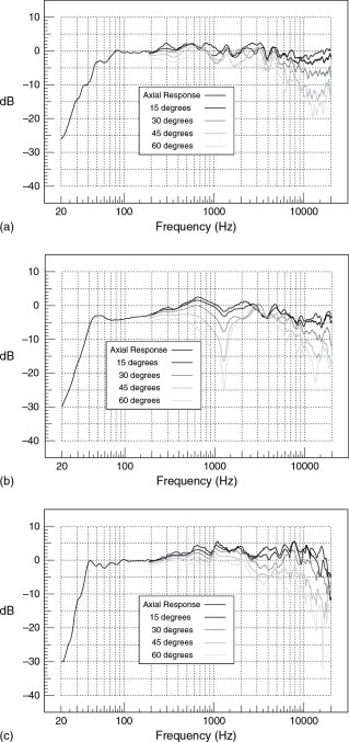
Figure 19.2 Horizontal directivity, (a) LSR-32, (b) BBSM-5 and (c) System 600A

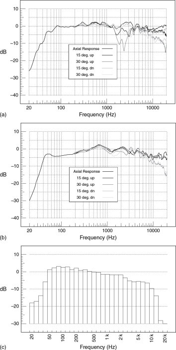
Figure 19.3 Vertical directivity of JBL and Westlakes plus total power response of Tannoy 600A. (a) LSR-32, (b) BBSM-5 and (c) Total power of System 600A

The horizontal off axis response of the JBL LSR32 is extremely well behaved. Indeed, the LSR in the name refers to ‘Linear Spatial Reference’, because the loudspeaker is designed especially to yield a smooth reverberant response in typical rooms. Even up to 60° off axis, the response differs from the on-axis response only by a gradual high frequency roll-off. The vertical directivity is similarly well controlled (Figure 19.3(a)), except for the sharp dip around 2 kHz in the ‘30° up’ direction. To maintain this sort of response with non-collocated drivers implies superb engineering and forethought. Almost nobody is going to listen from 30° above the loudspeaker, and the reflexions from that direction are likely to be innocuous in well-designed listening rooms. In fact, in many control rooms the ceiling is relatively absorbent, so the energy travelling 30° up is not likely to contribute anything significant to the room sound. The crossover has no doubt been carefully designed to push that cancellation node into the least problematical direction.

The Westlake exhibits an entirely different approach. The 30°-up dip in the frequency response of the JBL is due to the crossover design and the physical path length difference problems outlined in Figure 13.11. The Westlake uses a horizontal driver alignment, so if we look at the horizontal directivity of the BBSM-5 (Figure 19.2(b)) we notice the cancellation dips that are evident in the vertical directivity plots of the JBL. The notches are quite severe, but they may be more pronounced than normal due to the on-axis dip at the same frequency, 1200Hz. The vertical directivity of the Westlake is excellent due to the low mounting of the tweeter, which puts it no more than about 10 cm above the line passing through the centre of the bass drivers. At the crossover frequencies therefore, when all three drives are operating together, they are more or less horizontally in line. This type of arrangement is good from the point of view of not obstructing the main monitors when the small ones are mounted on stands behind a mixing console, or on the meter bridge, but it does cause the response to change with horizontal movements of the listener, as described in the previous chapter. Sharp response dips of this nature do not tend to be very audible, which is fortunate because they are an unavoidable result of spaced driver geometry, but the Westlake dip is quite broad.

In fact, the JBL allows the front panel, which holds the tweeter and mid-range driver, to be rotated through 90° for horizontal (landscape) mounting of the cabinet if desired. However, the sheer size of the cabinet, almost 40 cm in width, would still make it rather too large for meter-bridge mounting if the main monitors were not to be obstructed. The vertical notch at 30° up would still remain because it is related to the mid-range and tweeter interference. Where the loudspeakers are used as the principal monitors, of course both options are available.

The Tannoy avoids all of these problems by means of its dual concentric construction. The tweeter fires through the centre of the woofer, which it uses as its horn flare. The concentric design means that the horizontal and vertical directivities are equal, because there is no physical off-set of the drivers which can create cancellation at the crossover frequency. The Tannoy off-axis response shows a gradual fall in upper-mid frequencies that is perhaps slightly more than is the case with either the JBL or the Westlake. However, the Tannoy exhibits a slightly rising on-axis high frequency response, whereas the other two have somewhat falling responses. There is an old hi-fi trick, described in Chapter 11, which is to boost slightly the on-axis high frequency response to try to flatten the total power response at the listening position, compensating for the ‘darker’ reverberant room response caused by the off-axis roll-offs. The subjective effect of this is highly room dependent. As the horizontal and vertical directivity plots of the dual concentric design are identical, and are both as shown in Figure 19.2(c), Figure 19.3(c), shows the total power response for the Tannoy System 600A, which is very smooth indeed. The on-axis rising response no doubt contributes to this.

The price to be paid for the use of dual concentric drivers is that the tweeter horn is being modulated at high levels of low frequency output, and the driver design is more complex. The former may lead to a rather idiosyncratic, level-dependent sound, and the latter may force other design compromises that would perhaps not be desirable had the co-axial requirements not existed. Nevertheless, Tannoy are one of the true long term players in the studio monitor industry, with over 60 years of fully professional acceptance, and they perhaps know more about dual concentric driver design than anybody else. Indeed, Tannoy registered the description Dual Concentric. If the System 600A is mounted horizontally or vertically, it performs in an identical manner.

19.5 Acoustic Source

The acoustic source represents the distance behind the baffle from which the different frequencies appear to emanate. Obviously a big change in the acoustic source at low frequencies will cause them to arrive noticeably later than the higher frequencies, which causes the time-smearing of transients. As sound travels at around 340 metres per second, each metre of displacement will cause an arrival delay for the affected frequencies of about 3.4ms. The acoustic source shift is due to group delay in the electro-mechanical filters, which results from the electrical crossover roll-offs and the associated roll-offs of the drivers and their associated ports and cabinets. For any given frequency, the steeper the roll-off, the greater the group delay. (See Glossary.)

Figure 19.4 shows the acoustic source plots of the three loudspeakers. As mentioned in Section 19.2, the JBL has a third-order low frequency roll-off, the Westlake a fourth-order roll-off, and the Tannoy a sixth-order roll-off. Not surprisingly, it can be seen that at 40Hz, the JBL has an acoustic source almost 2 m behind the baffle, the Westlake 2.4 m, and the Tannoy over 3 m, the latter representing over 10ms of signal arrival delay for the low frequencies relative to the high frequencies.

The audibility of these time shifts is not well understood, but the consensus is that the sound is more natural if the group delays (the phase shifts) are kept to a minimum. The late Michael Gerzon, one of the most respected audio investigators of the twentieth century (co-inventor of the Soundfield microphone, Ambisonics, the Meridian Lossless Packing data compression system, and the first proponent of dither noise shaping), was of the opinion that for natural sound reproduction, the minimisation of phase shifts down to 15Hz was more important than the maintenance of a flat amplitude response down to much higher frequencies. Figure 19.5 illustrates the idea diagrammatically, with the low order roll-off of the (a) curve tending to sound more natural, despite rolling-off from a higher starting point than the (b) curve. In general, the subjective audibility of the low frequency roll-off order in small loudspeakers still needs much further investigation.

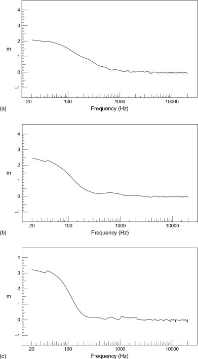
Figure 19.4 Acoustic source plots, (a) LSR-32, (b) BBSM-5 and (c) System 600A

Figure 19.5 (a) The plots in this figure show three very different bass responses. Despite imparting very different tonality or timbre to the music, they could nonetheless all be perceived as having subjectively the same ‘quantity’ of bass, as related to mid and top, if their responses above 500Hz were all the same. This, however, would be highly dependent upon the nature of the musical signal. In general, the rock world tends to favour something akin to the ‘b’ line, the classical world the ‘a’ line, and many cheap domestic systems the ‘c’ line. (b) Plot ‘a’ is typical of many good quality small, free-standing loudspeakers, such as are frequently employed as close-field monitors, on top of or immediately behind the mixing console. Plot ‘b’ would be typical of a large, high quality, built-in monitor system. Clearly there will be more overall bass energy produced by ‘b’ on a musical signal possessing a wide-band low frequency content, but on much popular music, the perceived balance between bass instruments may be remarkably similar when heard via either of the two curves

19.6 Step-Function Responses

Figure 19.6 shows the step-function responses of the three loudspeakers. The perfect step-function response would be as shown in Figure 19.7. For the tail not to slope downwards, the response would need to extend flat to DC, so the steepness of the decay slope is a function of the low frequency response of the loudspeaker system. It could only be horizontal if the loudspeaker box was sealed and placed in an airtight room. The spike at the beginning of the JBL response in Figure 19.6(a) is the tweeter, which can be seen to respond a fraction in advance of the mid range drive unit, which is represented by the second, higher peak. The third, more rounded peak, at around 3.5 ms, is the  woofer. This time non-synchronicity is due to the physical alignment of the drivers and the group delay due to the crossover frequency and slope. The manufacturers considered the subjective effect to be too small to warrant complicating the design.

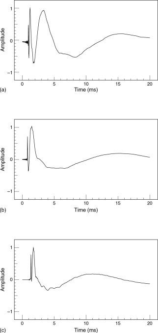
Figure 19.6 Step-function (Heaviside function) responses, (a) LSR-32, (b) BBSM-5 and

(c) System 600A

Figure 19.7 A step function

The Westlake shows in Figure 19.6(b) a more compact response. The tweeter can still be seen to speak in advance of the woofers, though only by about 500 microseconds. The response can be considered good. The time separation of the drivers at the crossover point also manifests itself as a kink in the acoustic source plot, Figure 19.4(b), at around 800Hz. The Tannoy shows a better step function response, this time with only about a 200-microsecond delay, which is probably inaudible. However, for comparison, Figure 19.8 shows the exemplary step function leading edge of two Quad Electrostatic loudspeakers, which shows what can be achieved.

Figure 19.8 (a) Step-function response of a Quad Electrostatic Loudspeaker (ESL). (b) Step-function response of a Quad ESL63, but on a much shorter timescale than (a), showing an almost perfect leading edge

19.7 Power Cepstra

The power cepstrum responses highlight problems due principally to surface irregularities and diffraction. The power cepstrum plot of the JBL, in Figure 19.9, shows almost no evidence of reflexions, which suggests that the stereo imaging should be good due to the lack of physically-separated secondary diffraction sources. The cepstrum plot of the Westlake shows evidence of echoes at 0.2 and 0.5 ms, and these may be responsible for the slightly irregular frequency response in the mid-range, due to interference between the direct and secondary sources (see Chapter 4). The Tannoy shows evidence of reflexions at 140 and 280 microseconds (0.14 and 0.28 ms) which may be due to the discontinuities in the horn flare where the metal phasing plug meets the coil gap of the low frequency cone. Again, these could be the source of some of the on-axis mid-range frequency response irregularities.

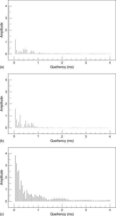
Figure 19.9 Power cepstrum, (a) LSR-32, (b) BBSM-5 and (c) System 600A

19.8 Waterfalls

Figure 19.10 shows the waterfall plots for the JBL, the Westlake and the Tannoy. Waterfall plots display time, frequency and pressure amplitude in a three-dimensional form. The most noticeable difference between the plots is the greater low frequency overhang of the Tannoy. Although the decay of the Westlake ultimately falls below the −40dBIntermodulation distortion at higher level more rapidly than the JBL, there is much more initial energy in the decay below the 100Hz region. The steeper roll-off of the low frequency response of the Tannoy results in more ringing energy in the filters. The more resonant a filter, the sharper will be its Q and the longer it will ring. A highly tuned bell rings longer than an old metal barrel. When the note is more defined, or the filter slope is steeper, the result will be a longer ‘ring-on’ time, or resonant hangover. The time response of a loudspeaker system cannot be separated from the roll-offs in its frequency response. Therefore, for the best transient response, the frequency response must be as wide and as flat as possible. With many active systems like the Tannoy System 600A, however, the need for low frequency driver  protection in such small boxes gives rise to the need for steep protection filters, but the time response suffers accordingly. The time response of the Tannoy, at low frequencies, can be seen to go completely off the scale.

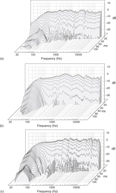
Figure 19.10 Waterfall plots, (a) LSR-32, (b) BBSM-5 and (c) System 600A

19.9 General Discussion of Results

The three loudspeakers under discussion in this chapter were chosen because they are all good performers. They are all above average in the range of loudspeakers typically used in professional studios as close or mid-field references. Despite this, no aspects of their performances match. Neither their pressure amplitude responses, phase responses, time responses, harmonic distortion responses, nor their diffraction characteristics need an expert to separate them. They are all obviously different. It is therefore not difficult to conclude that the loudspeakers all sound different; which they do.

A parallel exists with microphones, which are more or less loudspeakers in reverse. Nobody would pay €3000 for an old Neuman microphone if a €200 Shure could be equalised to sound the same. The characteristic sounds of electro-mechanico-acoustic transducers are highly complex combinations of the convolution of their time and frequency domain responses, along with the spacial responses, which also affect their overall responses in non-anechoic conditions. One great problem for investigators looking into the audibility of various aspects of loudspeaker performance is that of separating combined effects. Where a diffraction problem causes spacial smearing by introducing secondary sources, then what is being heard? The time domain effects, the frequency domain effects, the spacial effects, or the combinations? Despite all the money involved in the music, hi-fi and recording worlds, an absolutely extraordinarily small amount is spent on subjective/objective correlation. This is a sad reflection on how the professional industries have been usurped by the business people.

The current situation is that there is no loudspeaker that is optimal for all rooms. This fact can be clearly seen from the on and off-axis responses of the three loudspeakers studied in this chapter. No loudspeaker is optimal for all music. Of the three types of low frequency responses shown in Figure 19.5(a), one really would not want to play classical music through ‘b’ or disco music through ‘a’, because they would simply sound much more appropriate in the reverse order.

Obviously, no loudspeaker can sound optimal in a bad room, though the Tannoy would probably sound better than the Westlake because of its very smooth total power response, as shown in Figure 19.3(c). All the designs are affected very differently by their circumstances.

High definition monitor systems with low distortion, good transient accuracy, flat and extended frequency responses, high SPL capabilities and decent sensitivity are expensive to make and require expensive components. They also tend to be large. Commercial realities therefore force compromises on loudspeaker designs, and the wide range of loudspeakers that are commercially available reflect the need for choice if best-fit compromises are to be economically matched to circumstances. Unfortunately, the people who choose the loudspeakers are rarely fully familiar with the reasons for the compromises. They hear a loudspeaker in one set of circumstances, presume that the sound quality is the responsibility of the loudspeaker, alone, and then wonder why they sound different in another environment. This is why for the highest quality of reproduction, the loudspeaker system and the room should be designed as one entity.

All this makes it even stranger that a loudspeaker of seemingly dubious quality, such as the Yamaha NS10M, has found favour as a workhorse in such a wide range of environments, but with close inspection, reasons can be found. In fact, it may help to put some of the subjects discussed so far in this chapter into a useful context if we try to correlate the subjective and objective characteristics of a loudspeaker as well known as the NS10M. After the cessation of production of the loudspeaker in 2001, a series of interviews were made on behalf of Studio Sound magazine, and were published in August of the same year.⁵ What follows in the next section are excerpts from those interviews, which will hopefully throw some light on to why they were so widely used. Section 19.11 will then try to match their performance characteristics to the comments of their uses.

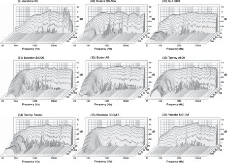
Figure 19.11 More waterfall plots. Note the rapid decay of the 5C and NS10M

19.10 The Enigmatic NS10

In the 1960s it was customary for ‘pop’ record producers and engineers to check what a mix would sound like on a ‘transistor radio loudspeaker’ before approving it. It was generally believed that what people heard on the radio had a big influence on whether they bought a record, or not. Radio was a big influence on sales, and the consoles such as the Neves of the late 1960s had small, built-in loudspeakers, which in many cases could be used as a radio reference.

As awful as these things were, and to a large degree they were not really representative of anything, they did sometimes help to get a more appropriate balance between guitars, vocals and reverb levels. They were very inconsistent though, and recording engineers were always complaining about them. People then moved on to making a Compact Cassette and playing the results back on a domestic machine, either inside or outside the studio. Somewhere in the early 1970s, there appeared a new ‘reference’ loudspeaker, the Auratone ‘Sound Cube’. These relatively tiny loudspeakers could produce prodigious output levels when driven by Crown D150 amplifiers, or similar. Their small size also caused very little obstruction of the main monitors if they were mounted on the meter bridge of a mixing console. The fact that they were single driver loudspeakers ensured a smooth phase response through the vocal region, and this no doubt contributed to their usefulness, because crossovers in general simply will not sum their outputs to give an accurate reproduction of the input.

The Auratones reigned supreme for almost a decade, although not everybody used them or liked them of course, but in the early 1980s, there came a challenger, the NS10M. Designed as a home hi-fi loudspeaker, it was generally badly received by the critics, but this little loudspeaker had a rock-and-roll punch which caused many people in the recording industry to take note. It was also reasonably robust. The thing that puzzled so many rival loudspeaker manufacturers for the subsequent 20 years had been why it was so popular. What characteristics did it have that led so many people to have confidence in the fact that the mixes that they did on them would translate well to the street? A number of well-respected people from the music industry were therefore asked to give their opinions about the NS10s, in the hope of getting a little more insight into what made these loudspeakers so special.

The first person to be approached was Bob Clearmountain, one of the great exponents of the NS10s. He said that in the early 1980s his favourite mixing loudspeaker was the KLH17. The problem with them was not their sound, but their fragility; they just would not withstand the punishment of studio use. He was then introduced to the NS10 in its early domestic form, and was impressed by the way that the mixes travelled. The only problem was that the mixes lacked top outside of the studio, so toilet paper placed over the tweeters was used as an acoustic filter, to reduce the high frequencies perceived during mixing. Apparently, this worked well, because his mixes then did not surprise him when played elsewhere. When the NS10M ‘Studio’ version came out, the toilet paper was no longer necessary, and the NS10Ms were then his mainstay for many years.

What had puzzled the interviewer for years was how INXS’s Devil Inside could sound so well balanced on wideband monitor systems, in good rooms, when Bob had claimed to have only monitored the mix on NS10s. One problem with the use of close-field monitors, only, is that people often have a tendency to make changes to the bass and bass drum levels and equalisation, according only to the limited frequency range that they can hear. It is a common complaint from mastering engineers that if these have been wrongly judged on small monitors, there is often nothing that the mastering houses can do to repair the situation such that things will still sound well balanced on full-range systems; be they in a home or a studio environment. Bob solved the mystery by paying great tribute to Chris Thomas, the recording engineer. It seems that the multitrack recordings, which had been checked on large monitors, were of such quality and freedom from problems that Bob’s job was mainly to balance the relative instrument and effect levels. The quality control had already been done for him. He recognised that he was in the fortuitous position of normally only working with high quality artists and recordings. Principally he is a mixing engineer, rather than a recording engineer. He trusted the NS10s for so many years because they were the tools that helped him do his job. ‘They helped to pay my rent’, he said, ‘because I could have confidence in the work that I did on them. I’m not a very technical guy, I’m a music mixer, and I use the tools that I can work with best. Why they work is not too important to me’.

The next person to be spoken to was Alan Douglas (the Grammy winning engineer of the Riding with the King duet album of B. B. King and Eric Clapton), on the day before he was starting recording with Annie Lennox. He said that he thought that NS10s sounded hideous, but they had a rock-and-roll sound, which if you got used to it could lead to good results from a mix. Alan said that the Quad amplifier/NS10M combinations, often used in the UK, was something that he found very difficult to deal with, but the NS10s on a large Crown amplifier was something that he had achieved good results with. Like Bob Clearmountain, Alan’s current preference is for KRKs, but he also had used the Auratones many years ago. ‘If you can get a mix to sound good on an Auratone, then you know you’re really in business’, he said. He prefers the KRKs because they can still, despite their size, get a good control room ‘buzz’ for the musicians. At home he likes to listen on Tannoys, but he finds it difficult to work on them in a studio. On the other hand, the loudspeakers that he can work with in the studios he does not like for home use. Such are loudspeakers!

Nick Cook had spent much of the previous ten years as the head of Fairlight’s European operations, and as Sales Director of Amek. From the mid’70s though, he was a busy recording engineer, working in some of Britain’s best facilities.

I always used to check the core sound on the large monitors, then do the equalisation and balancing on the NS10s. They are bright and harsh, and the old ones without the ‘loo’ roll led to too little top on the mixes. The change from the old domestic NS10M to the NS10M Studio version caused a short period of confusion, because the reference changed, but the sound had essentially the same character and people soon adjusted.

Nick believed that the recording and mixing processes require very different loudspeakers.

During the recording you need to hear the instruments in detail, whilst at the same time being able to inspire the musicians to great performances. The subtleties of fine balance are not important at that stage. By the mixing stage you should already have well recorded multitracks, so the mixing process becomes more a question of balance.

Nick also believed that one asset of the NS10 over many other of its contemporary loudspeakers, when it was first used in studios, was its ability to accept a ‘solo’d’ bass drum without expiring. ‘They also sounded good when sitting on the top of SSL consoles, and once their reputation had been established in such a position, and they had been used on “top” recordings, the industry in general saw them as a reference’. Nick also commented on the solidity of the NS10 cabinet construction, which ensured that the cabinet, itself, was not audible. There was thus, no boxy sound, which helped it to have more of the character of built-in monitors. Furthermore, the solid cabinet did not tend to excite mixing console resonances, which could be a problem with some of the NS10s more flimsy rivals. ‘What I’ve also noticed’, he said, ‘is that the general sound of recordings has changed over the years, and some of the reason for that could have been that the most popular mixing loudspeakers begin to set their own standards for what is perceived to be right’. What you become accustomed to becomes a de facto reference in the absence of any clearly defined industry reference.

Now over to the man from the ‘Beeb’. Although Chris Jenkins had worked for SSL for the previous 20 years, he was BBC trained and spent some years with Virgin. He has been generally well respected as a musician, recording engineer, maintenance engineer and console designer. Surely, he must have some insight into the popularity of the NS10M. ‘I used to be able to perceive a lot of dynamic detail on the Auratones’, was his first comment. His technique was to get a clean recording by using the main monitors, then switch to the NS10s or Auratones to get a balance between the instruments. ‘Once you learn to trust the balances that you get on a certain loudspeaker that you can rely on, then from the engineering point of view there is really no need to know why – you just get on with it. I tended to prefer the Auratones to the NS10s,’ he said, ‘because I got more of a sense of the dynamics; perhaps due to the fact that it was a single loudspeaker with no crossover’. Somewhat surprisingly, not only could a person as musical and technical as Chris not put his finger on the ‘why’, but he did not even seem to care. Only the results counted.

The next person to be approached was Mick Glossop, the producer-engineer of artists such as Frank Zappa, Van Morrison, and Sinead O’Connor. Mick was continuing to use both NS10s and Auratones. ‘I don’t really discuss what or why with other people, because it is only the results that I get that count’, he said. I then read him the quote from George Massenburg, mentioned elsewhere in this book. To recapitulate, Massenburg had said ‘I believe that there are no ultimate reference monitors, and no “golden ears” to tell you that there are. The standards may depend on the circumstances. For an individual, a monitor either works or it doesn’t. . . . Much may be lost when one relies on an outsider’s judgements and recommendations’. ‘Absolutely!’ was Mick’s reply. In fact, the George Massenburg quote had been tested on several other people during these interviews, and they all agreed that he had (as is his tendency) hit the nail right on the head.

Mick went on to say

If things sound too good on the loudspeakers, then it makes you lazy and you don’t work on the music. You then take things home and realise that you could have, and should have, done a lot better. I use large monitors, from time to time, to check the bottom end, but often I do whole recording sessions on NS10s. I really don’t like them at home, though; they’re for work only. I have often noticed that during the mastering, I need to add something around 2.8 kHz, because I tend to undermix those frequencies when using NS10s. I still use Auratones to set the bass and vocal levels in a track. I can also hear distortions better on the Auratones, and they have a lot of detail when quiet. I can get a good balance on Auratones which works well when switched to NS10s, but I won’t use the Auratones from scratch. I dread having to change monitors, because I have become so used to the ones which I use. If I had to change, I would probably go to KRKs, but I also really like the Questeds, I can work well on those. I use large monitors when available as a low frequency check, but if I don’t know the room that they’re in, it can be misleading. Essentially, though, I want to put all my energy into the mix, and I don’t want to have to waste time thinking about the loudspeakers.

Finally, here are the comments from the London-based songwriter/engineer/ producer/studio owner, Michael Klein.

What I like about working on the NS10s is that they make the mid-range very clear and prominent. This is normally where many instruments are fighting for the same space. The NS10s allow me to concentrate on getting the mid-range finely balanced, and once that is done, the basis of a mix is usually well established. I wouldn’t record on them, though, and I certainly wouldn’t want them at home, but for mixing, they are a great help.

So, with all those words of wisdom from such esteemed recording engineers, where does that leave us? Well, it seems that none of them are the slightest bit interested in loudspeaker design – they just want to use the ones which work for them. They all also appear to agree with George Massenburg’s statement. They almost universally saw the NS10M as a mixing tool, not a recording monitor, and it is perhaps in this area where so many small studios miss the point. They see top name engineers using NS10Ms for mixing but fail to realise, firstly, that they often use large monitors during recording, and, secondly, that they are immensely experienced people who can rely on that experience to interpret what they are hearing. They are perhaps not taking what they hear to be gospel, but are interpreting what they hear in the light of their experience.

The people interviewed all used the monitor systems that worked for them, and they all tended to agree that they wanted to use loudspeakers that made them work hard at a mix. Interestingly, there was a general rejection of a very popular brand of powered loudspeakers because they did not make bad mixes sound bad enough. This was summed up by Alan Douglas’s comment that ‘If you can make a mix sound good on Auratones then you know you’re in business’. Not one person spoke about frequency response, or hardly any other technical aspect of performance. They all spoke in subjective terms, even though some of them have deep technical knowledge. However, this lack of accurate, descriptive feedback to the manufacturers has not helped the further development of monitor systems, and that communication gap between users and manufacturers still exists.

Well, as the author, I suppose that I ought to add my own comments, from my points of view as a former recording engineer and producer, and now, principally as a studio designer. My career as a mainstream recording engineer and producer was largely coming to an end when the NS10 was first introduced, but, in the years since, I have always been around studios and recording personnel. In fact, understanding the needs of other engineers is perhaps a greater part of my job now, than ever it was before. My own opinion of any monitor is not that it should sound nice, but that it should scream in your face when things are wrong. This philosophy is borne out by the number of top producers and engineers who, when relaxing at home, absolutely do not want to listen to the loudspeakers that they work with. They want to hear the problems smoothed over when listening for pleasure, at home. [Though, as always, there are some exceptions.]

What has been discussed in this section are the subjective opinions about why the people interviewed have elected to use the NS10Ms. What has not been discussed, however, are the aspects of the NS10M’s performance that may be responsible for its widespread use. The following section will now attempt to highlight those aspects of performance, in objective terms, which correlate well with the subjective comments. The work is based on a paper presented to the Reproduced Sound 17 Conference of the UK Institute of Acoustics in November 2001.⁶

19.11 The NS10M – A More Objective View

The original NS10M was conceived as a domestic hi-fi loudspeaker for bookshelf mounting. As such, it was not a great commercial success, and neither was it very well received by the international hi-fi press. However, it was readily adopted by many recording personnel as a close-field studio monitor for rock/pop mixing. It effectively took over the mantle that had largely been carried by the Auratone 5C ‘Sound Cube’. Despite the output of the Auratone being prodigious for its size and era, its limitations had led many users to seek other loudspeakers with higher output levels and wider frequency ranges. Nevertheless, many of them still sought loudspeakers that exhibited the more valued characteristics of the Auratones. The NS10s were widely considered to fill that need.

The original NS10M fell short of the requirements on two counts; firstly, it was still somewhat lacking in output capability, and secondly, it was considered to have an excess of high frequencies. The former problem gave rise to the need for frequent driver replacements, whilst the latter was commonly solved by the fixing of a piece of toilet paper over the tweeters. The old tale about the discussions over which brand was most appropriate, and whether one sheet of two was required, was not a joke; such discussions actually did take place. Yamaha subsequently dealt with both problems with the introduction, in the mid-1980s, of the ‘NS10M Studio’, hereinafter simply referred to as the NS10M.

19.11.1 Specifications and Measurements

The NS10M is a two-way loudspeaker consisting of a 180 mm paper coned low frequency driver and a 35 mm soft domed tweeter, all in a 10.4 litre sealed box. The crossover is second-order passive with asymmetrical turnover frequencies and in-phase connected drivers. The frequency range is quoted as 60Hz to 20 kHz, the sensitivity is 90dB for 1 W at 1 m, and the maximum (peak) input power is rated at 120 W. The crossover frequency is 2 kHz and the nominal impedance is 8 Ω.

Measurements carried out by Dr Keith Holland at the ISVR revealed a frequency response with a deviation of ±5dB over the range from 85Hz to 20 kHz under anechoic conditions. This would hardly seem to be impressive in itself, but closer examination shows that this deviation is due to an inverted ‘V’ characteristic response shape rather than the irregular wiggles exhibited by some loudspeakers.

Figure 19.11 shows a selection of nine of the 36 waterfall plots published in Reference 6, and reproduced in Appendix 2 at the end of the book. The nine plots represent the last eight of the alphabetical order of the 36 plots, plus the Auratone. The two outstanding features of the Auratone and NS10M are the inverted V response shape, and the very rapid response decay over the entire frequency range. Both of these characteristics are largely due to the sealed box nature of the designs. We will return to this point in the concluding part of this section, but suffice it to say that of the 36 waterfall plots depicted in Appendix 2, the only other loudspeakers exhibiting a similarly rapid response decay were the ATC SCM20A, the AVI Pro 9, and the M&K MPS-150.

Figure 19.12 shows the step function responses of the same nine loudspeakers. All of these are very good compared with many typical monitor loudspeakers of 25 years ago. The Auratone exhibits the more exemplary rise because of its single driver nature. The separate peak of the tweeters responding early can be seen in most of the other plots. The Yamaha shows a better than  average step function response, which is a good indicator of its transient performance. The response tail is also well damped, which corresponds with the rapid decay shown in the waterfall plot.

Figure 19.12 Step responses. Note the rapid damping of the tails of the 5C and NS10M

An electrical input signal having a step response is shown in Figure 19.7, but for anybody not familiar with it, a battery connected to the loudspeaker  terminals via a switch can also be used as a crude source of a step function. Rise time, simultaneous response of all drive units in a system, and ringing in the decay tail are things that step functions show up well.

Figure 19.13 shows the harmonic distortion performances of the same nine loudspeakers as in Figures 19.11 and 19.12. Again, neither the NS10M nor the Auratone are bad performers. This is made even more emphatic when one considers that the other seven loudspeakers (and the other 34 if one looks at the full presentation in Appendix 2) are all of reputable make and are all designed for professional use.

Figure 19.13 On-axis frequency response and distortion

19.11.2 Discussion of Results vis-à-vis Subjective Perception

It is widely considered that a reference monitor loudspeaker should exhibit a relatively flat frequency response. However, it should be remembered that the loudspeaker and its mounting in a room are part of one system. It is the frequency response of that system which really needs to be flat in order for the recording personnel to perceive an accurately frequency balanced representation of the music being recorded. The free-field response of the loudspeaker is not what is heard in a control room. The following four figures may help to clarify this point.

Figure 19.14 shows the response curves of an idealised loudspeaker of approximately similar size to the NS10M, both in free-field conditions and  flush mounted. Figure 19.15 shows the response of an NS10M suspended in the open air, about four metres from the nearest reflective surface. The response wiggles are due to the reflexions from the nearby surfaces, but the overall shape can be seen to be very similar to the free-field response shape in Figure 19.14. Figure 19.16 shows an NS10M mounted on top of the meter bridge of a mixing console, both suspended in mid-air. Additional comb filtering of the response is evident due to the proximity of the top surface of the mixing console, but the overall trend is that of the flattening of the bass response. Figure 19.17(a) shows the response of an NS10M on top of the meter bridge of a mixing console in a room typical of many recording studio control rooms. Despite the extra irregularities due to boundary reflexions, the overall trend of the low frequency response shape is in the direction of the flush mounted response shown by the dashed line in Figure 19.14.

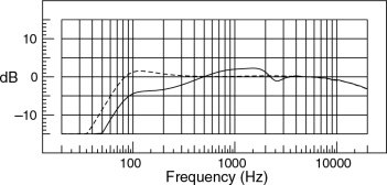
Figure 19.14 Response of idealised loudspeaker: flush-mounted (---) free-field (—)

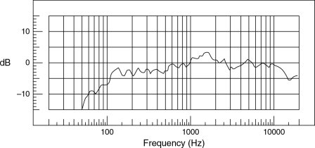
Figure 19.15 Response of NS10M, flown from a crane, 4 m above the ground and 4 m from the nearest wall. Measurement taken outdoors

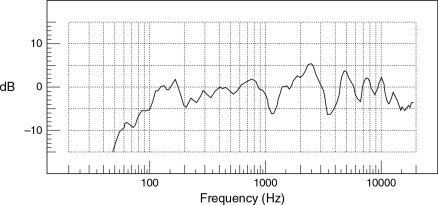
Figure 19.16 NS10M, mounted on the meter bridge of a mixing console, both flown from a crane, outdoors, 4 m above the ground and 4 m from the nearest wall

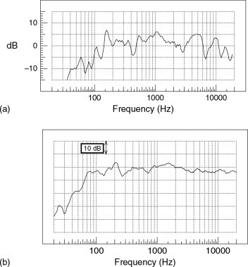
Figure 19.17 (a) Pressure amplitude response of an NS10M, on top of the meter bridge of a mixing console, in a room of about 30 m², containing material typical of a small studio control room. (b) Actual response of an NS10M in a small studio, placed directly against a wall, with no mixing console beneath it. In effect, the bookshelf mounting for which it was originally designed

In Section 19.10, Nick Cook was quoted as saying, ‘They also sound good when sitting on top of SSL consoles’. Although he was referring specifically to SSL consoles, he actually acknowledged that they worked well on other consoles, also. It is worth noting, though, that the structure and shape of the console on which they are mounted will affect the response, and perhaps it is likely that the more solidly built consoles, like the SSLs, will colour the sound less than would be the case with lighter, more resonant consoles. The implication is also that the NS10Ms first established their reputation on  the better consoles, on which they also tended to sound best, and that once their use had been established in the ‘first division’ they were then seized upon by the lower echelons. Nevertheless, Figures 19.14–19.17 do seem to reinforce the concept of the NS10M, plus a mixing console and a typical control room, yielding an overall frequency response of a nature that many recording personnel appear to need to hear. That the mixing console plays its part in the response is perhaps reinforced by the number of people who work daily with NS10Ms but who do not choose to use them at home – where large mixing consoles are usually conspicuous by their absence.

The mid-range response peak, which is clearly observable around 1.7 kHz in Figures 19.11 and 19.15, appears to be responsible for the ‘harsh’ description that is often referred to when discussing the NS10M. This could objectively be considered a negative asset. However, during the interviews quoted in the previous section, Michael Klein said ‘What I really like about the NS10Ms is that they make the mid-range very clear and prominent. This is normally where many instruments are fighting for the same space. The NS10Ms allow me to concentrate on getting the mid-range finely balanced, and once that is done the basis of a mix is usually well established’. Many people would no doubt echo Michael’s comments. His words again highlight how the NS10M has been seized as a tool to help to get a job done.

Certainly in terms of frequency response, the NS10M appears to have a free-field response which, when in the typical surroundings of a recording studio, gives many people what they need in order to get a job done. The relatively low distortion no doubt also helps.

But what of the time response? Let us now turn again to the waterfall plots of Figure 19.11. Again, during the interviews recounted in Section 19.10, several people referred to the ‘rock and roll punch’ or the ‘rock and roll sound’ as Alan Douglas was quoted as saying. This clearly relates to the rapid decay of the NS10M. Two other things can also be said to result from the time response. The first is that the rapid decay is reminiscent of many good, large monitor systems in well-controlled rooms. Such systems often have cabinet resonances tuned way down below 30Hz, and they are usually without any protective filtering in the audio frequency band. The tuning ports and protection filters that are typically inside the lower bass region on smaller loudspeakers give rise to the low frequency ringing which is typical of most of the plots shown in Figure 19.11. The NS10M has neither tuning ports nor protection filters. The tightness of the bass, however, can be influenced by the amplifiers driving the NS10Ms, and powerful amplifiers with extended low frequency responses should be used if the full potential punch is to be realised. High instantaneous current delivery is also important.

The second point is that the rapid decay of the low frequencies from the NS10M is less likely to cause confusion by distorting the time responses of the bass drums and bass guitars. One repeated complaint from many mastering engineers is that people who mix on a variety of small monitors often get the bass/bass-drum ratio wrong. As these exist in the same frequency range, an inappropriate balance between the two can often not be resolved by equalisation (or any other process) at the mastering stage. It is probable that fast decays are less likely to lead to such erroneous relative balances. After many investigations there is now growing evidence to support this argument, because the obvious low frequency time-response differences shown in Figure 19.11 will inevitably convolve themselves with the musical instrument sounds. Determining which one is contributing what, during the mixing, may be all but impossible in the case of the loudspeakers with the longer decay tails.

19.11.3 Conclusions

From the above investigations, it would appear that the following statements can be made:

1. The free-field frequency response of the NS10M gives rise to a response in typical use that has been recognised by many recording personnel as being what they need for pop/rock mixing. The principal characteristics are the raised mid-range, the gentle top end roll-off (which is typical of many large monitor loudspeakers), relatively low distortion and a very short low-frequency decay time. The latter is aided by the 12dB/octave low-frequency roll-off of the sealed box design.
2. The time response exhibits a better than average step-function response, which implies good reproduction of transients.
3. The output SPL is adequate for close-field studio monitoring with good reliability.
4. They appear to mimic, in many ways, the characteristics of the good, large monitor systems (within their limited range) typically used in pop/rock recording, and hence they are recognisable to many recording personnel in terms of overall suitability for their needs.

Of course, the information presented here will only be deemed truly worthwhile if it can be used in the design of future loudspeakers for studio use. General acceptance of any such loudspeakers is, however, not merely a technological challenge. Widespread acceptance requires widespread exposure, which implies mass manufacture with good worldwide distribution networks and an affordable price. These are non-technical realities, which nonetheless affect the choices in today’s recording industry.

A strong implication from the data presented here is that loudspeakers that exhibit a flat free-field response will not have a flat response characteristic when placed on top of a mixing console in a control room. Many of the manufacturers of active loudspeaker systems provide significant ability (via d.i.p. switches and the like) to contour the low frequency response to the mounting conditions, yet it is remarkable in how many studios the switches are set ‘flat’ in a misguided belief that this provides the flattest response, even when mounting conditions dictate otherwise. However, one alarming result of looking at all 36 waterfall plots in Reference 6/Appendix 2, is the enormous variability in the low frequency time responses.

Another great controversy is whether it is wise to place the loudspeakers on the meter bridges or whether they should be on stands just behind the console. The latter system does tend to give a more open stereo imaging and less comb filtering, because of the reduction of desk-top reflexions. On the other hand, one then loses the bass reinforcement provided by the desk top, as shown in Figure 19.16. There are obvious compromises being made here. Clearly, though, it would seem that for optimum mounting behind the console, a design with a little more bass than the NS10M would be desirable. This subject is discussed further in Section 20.7.2.

It would therefore seem probable that the NS10Ms are so frequently placed on the meter bridges because that is where they have been found to exhibit their flattest overall response, even if some other aspects of their performance are compromised. The NS10M, almost certainly found a waiting gap in the studio monitoring market which it was reasonably well suited to fill. It had many of the characteristics needed for the then relatively unconsidered (in 1982) task of serious close field monitoring in rock/pop music studios. Nevertheless, whether by design or accident, it has made its presence felt in the music-recording world perhaps like no other loudspeaker to this day.

19.12 The Noise of Conflict

As discussed in Section 19.3.1, intermodulation distortion is probably the real enemy – the hidden enemy – that we fight when we try to reduce harmonic distortion. Dr Alexander Voishvillo, the Russian electro-acoustician, has recently been a driving force behind the search for a means of quantifying and comparing intermodulation distortion responses. His work is recommended reading for anybody who seeks to know more about the subject.^7–10

Total harmonic distortion gives the output response of a system to a single frequency input when the input frequency is filtered out. Spectrum analysers can separate the different harmonics, and sweep frequency analysers can display individual harmonics as a swept function of the input signal. Such plots are shown in Figure 19.1. Nevertheless, at any given time, the stimulus is a single frequency, and the measured products are multiples of that frequency. They are the very harmonics that would be produced by any acoustic instrument if a musician were to attempt to play a single frequency. The harmonics give rise to the tone colour (timbre) of an instrument. Harmonics are therefore musical sounds; in fact, they are the essence of rich musical sounds.

Why then do we measure harmonic distortion? The answer seems to be, ‘Because we can’. There is no doubt that it is a measure of the non-linearity in a system, but work over many years has shown it to correlate only poorly to perceived loudspeaker quality. Whilst it is true that the same mechanisms that give rise to harmonic distortion are the ones that are responsible for the intermodulation distortion, the latter is difficult to measure, because when every frequency modulates every other frequency, the variables seem to be endless.

There is also no magic ratio between harmonic and intermodulation distortion, because the intermodulation distortion depends on:

1. The absolute level of the signal
2. The bandwidth of the signal
3. The complexity of the signal
4. The peak-to-mean ratio of the signal
5. The waveform of the signal
6. The interaction between the above and a number of other factors, also.

Some instances may occur, in simple cases, where it could be said that, for example, the intermodulation products were three or four times the level of the harmonic products, which in many cases would be typical, but on complex musical signals, any seemingly fixed relationship tends to break down badly.

Intermodulation distortion in a non-linear system is therefore frequency dependent, level dependent, waveform dependent, . . . in fact, it is very difficult to devise any simple test signal that could yield a realistic description of how the intermodulation performance of two systems could be compared. In the words of Dr Voishvillo;¹⁰

Since the dynamic reaction of a complex non-linear system such as a loudspeaker cannot be extrapolated from its reaction to simple testing signals, such as a sweeping tone, the thresholds expressed in terms of loudspeaker reaction to those signals (total harmonic distortion [THD], [individual] harmonics, and two-tone intermodulation distortion) may not be valid.

That intermodulation distortion is the number one enemy of loudspeaker designers is probably true, whether too many of them realise it, or not. However, with such a characteristic nature that is constantly changing with the music, any useful presentation of its quality and quantity, numerical or graphical, must have a correlation to the psychoacoustic perception of the problem. Until now, no such credible presentation system has been widely accepted. So far, all attempts have been flawed, so intermodulation problems often tend to be ignored. Although the venerable Gilbert Briggs had so clearly identified it as a great problem by the early 1950s, the intervening years have not yet come up with any adequate quantification method.

The thing that must be borne in mind is that the intermodulation distortions (IMD) of complex signals tend towards being a modulation related noise. It is a little like trying to listen to a good hi-fi system whilst somebody is just outside the window using a chain-saw, whose noise production is dependent on the level and spectral density of the music, though not directly proportional to either. With IMD, transparency is lost, low-level detail is buried, and the sense of effortless reproduction cannot be achieved. Brass bands and choirs are great victims of intermodulation distortion. Their reproduction via loudspeakers can be very disappointing if one is accustomed to hearing them live. Whilst all the sources emanate from different points in space, the inter-modulation products are low, but when they are all mixed together and passed through a pair of loudspeakers, the intermodulation becomes obvious. This need not be a fault of the loudspeakers alone, because microphones are also often responsible for intermodulation distortion, and the electronic systems and digital converters can further add their products.

It must also be remembered that the air, itself, is also non-linear, and where very high SPLs exist, such as can exist in the throats of horns (be they trumpets or loudspeaker horns), intermodulation can be very evident. This is more evident in PA systems rather than at the levels normally experienced in recording studios, but nevertheless, in very large control rooms it can be a problem. Figure 19.18 shows the propagation distortion from a source at one-metre distance. Figure 19.19 shows the propagation distortion, for the same SPL at the measurement point, from a source at a distance of five metres. There is a strong implication here that for the same SPL at the listening position, the lower source SPL generated by a close-field monitor may produce significantly less IMD than that from loudspeakers at five metres distance, unless, that is, the loudspeakers at the greater distance generate significantly lower levels of non-linearities. In many cases, the exact opposite is the case, where the large monitors actually produce more non-linear distortion, level for level, than the ones used at close-range. Furthermore, where air propagation distortion is concerned, the greater distance travelled at high SPLs also gives rise to more distortion, so the generation of high SPLs from considerable distances seems to be a viable proposition only in studios with extremely linear monitor systems.

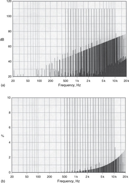
Figure 19.18 Multi-tone testing of intermodulation distortion. Propagation distortion in spherical wave, SPL 110dB at 1 m from the source. Radius of the source 0.5 m. First graph (a) isdB SPL, second graph (b) is per cent IMD to fundamentals. (Courtesy of Dr Alexander Voishvillo.)

Figure 19.19 Intermodulation distortion at higher level. Propagation distortion in spherical wave, SPL 110dB at 5m from the source. Radius of the source is 0.5 m. First graph (a) is dB SPL, second graph (b) is per cent IMD to fundamentals. (Courtesy of Dr Alexander Voishvillo.)

Figures 19.18 and 19.19 were based on a multi-tone testing system, where a whole series of tones are simultaneously injected into a system. The frequencies are chosen such as to maximise the separation of the intermodulation product frequencies, to help to see more accurately the spread of the problem. Inappropriately chosen frequencies could produce intermodulation products at the coincident frequencies, in which case some masking of the problems would take place. The multi-tone testing has shown that the total IMD can often be around four times greater than the measured THD. The implication is that in many cases, what people frequently believe to be harmonic distortion of music is actually, predominantly, intermodulation distortion. This helps to explain why there have been such poor correlations between measured THD and perceived distortion. The perceived distortion is more likely to be the IMD, which is neither being measured, nor adequately quantified.

What is more, various studies have shown that IMD can be irritating at only ten percent of the equivalent THD levels because of its inharmonic nature. Therefore, producing four times more of something, which is ten times more irritating, could suggest that the IMD problem is 40 times greater than the THD problem. It has even been shown, by using a fifth order static polynominal model, that non-linearity of the type 2f_i + f_j can be 34dB higher than the fifth harmonic distortion in the same system.

Voishvillo’s explanation for the extreme clarity that has been reported from the monitor system shown in Figure 19.20 is that not only are the independent recordings of the instruments not sharing any of the loudspeakers, but that they are also not sharing the same ‘air conduits’ between the loudspeakers and the ears. (The 16 loudspeakers are fed from separate tracks of a multitrack recorder.) At low SPLs, this idea of air conduits would violate the concept of the linear superposition of acoustic waves, but the non-linear interference concept has already been proved by experiment at high SPLs.

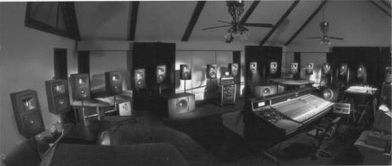
Figure 19.20 The multi-channel monitoring system in the private studio of Eugene Czerwinski, the founder of Cerwin Vega Inc. The use of one-track-to-one-monitor is said to reduce drastically the levels of intermodulation distortion, and to increase greatly the level of perceived openness and neutralness in the reproduced sound. (Photograph courtesy of Eugene Czerwinski.)

Normally, the harmonic distortion is measured by means of a fixed level signal, either static in frequency or swept. However, the non-linear distortions that relate to what we hear are the complex interactions within a complex, time-varying signal, and THD correlates poorly with this. Whilst THD is presented as a percentage of the signal, it could be that we are sensitive to absolute levels of IMD. We are accustomed to the harmonic density of instruments increasing as the musicians play louder, but somebody vacuuming in the room can be disturbing for the hi-fi listener whether the music is loud or quiet.

Anthony New published some interesting data in a pair of articles entitled ‘THD Is Meaningless’^11,12. Albeit taken from radio frequency amplifiers, he showed plots of the intermodulation products of two, three and four simultaneously applied tones, with a level about 65dB above the noise floor. On the two tone plot, four intermodulation products could clearly be seen above the noise floor. With three tones, nine intermodulation products were clearly visible, whilst with four tones, over 30 intermodulation products were evident. The IMD products increase rapidly as the number of stimulating frequencies increases, because the IMD products begin to intermodulate between themselves. One can easily imagine the result for a complex musical signal – a random-type modulation noise, perhaps only 40dB below the level of the music. His arguments are quite convincing.

To say that THD measurements are meaningless is perhaps going a bit too far, but to say that they are meaningless, in themselves, is probably fair comment. It is well known that many valve amplifiers produce much greater levels of second harmonic distortion than the better quality transistor amplifiers, without sounding distorted. A quick look at the tendency towards second order non-linearity generation may explain why this is so. In fact, the second order non-linearity produces no odd-order, unpleasant intermodulation of the f₁ ± 2f₂ nature. The products of the second order non-linearities tend to be fewer in number and lower in level than the higher order products. As just discussed, the higher order products can increase rapidly in both their density and cumulative level. They also tend towards a random noise type of frequency distribution, which the music cannot mask. (Note the black mass in Figure 19.19(a).)

When valve amplifiers produce second harmonic distortion it can be pleasant in moderation, but perhaps what is even more pleasant about such amplifiers is the lack of higher odd-order intermodulation products. This is perhaps also true of Class A amplifiers in general, which are free from crossover (zero-crossing) distortion artefacts at any level. In fact, it would appear that harmonic distortion is not a separate entity to intermodulation distortion, but is a special case of intermodulation distortion. If multiple tones are being used for intermodulation testing, and they are individually sweepable and all brought together in frequency, then when they blend together they will produce only harmonic distortion. Perhaps in this way it is easier to visualise that the same non-linear mechanisms give rise to both forms of distortion.

In electro-mechanical systems, such as loudspeakers, the non-linear restoring forces in the suspension systems are further sources of intermodulation and harmonic distortions. However, the deflexions of these suspensions under musical drive can be complex in the extreme, and they bear little relationship to the electrical factors that give rise to non-linearities in amplifiers, for example. This may explain why one per cent of second harmonic distortion may be excellent sounding from one device whilst being intolerable from another. It is therefore not the level of second harmonic distortion, in itself, which we are comparing, but the existence of other non-linear artefacts resulting from the different non-linear mechanisms or systems. Such mechanisms can also give rise to phase distortions of a dynamic nature, which can affect the stereo imaging. Another particularly nasty source of loudspeaker intermodulation distortion is magnet BL (force factor) non-linearity¹³, which can give rise to many more intermodulation distortion problems. Once again, though, these highly audibly unpleasant products may not be anywhere near adequately exposed by simple THD measurements.

Very much more work still needs to be done on the reduction of, and the meaningful measurement of IMD. One reason why there has been a lack of motivation by many commercial manufacturers of audio equipment has been that, because of the lack of accepted specifications, they have been reluctant to pursue expensive improvements that cannot be proved in the sales literature. A meaningful objective/subjective correlation measure would be a powerful stimulant to a global attack on the IMD menace. Nevertheless, it is probably true to say that the perceived clarity in any audio system is usually a direct result of the absence of intermodulation distortion.

19.13 Summary

The on-axis anechoic frequency response of a loudspeaker is not what will be heard in a control room.

Loudspeakers have many different physical layouts and will exhibit different directivity characteristics because of this.

Different on-axis responses may suit different mounting conditions. Harmonic distortion figures can be misleading, but they are an indicator for the existence of intermodulation distortions, which are probably the real culprits for any lack of musicality.

Steep low frequency roll-offs give rise to group delays that smear the time response of a loudspeaker.

Just as microphones of different designs cannot be equalised to sound identical, nor can loudspeakers.

Many recording engineers and producers use different types of loudspeakers for work and for pleasure.

Loudspeakers with anechoic pressure amplitude responses similar to the general shape of that of the NS10M tend to flatten when placed on the meter bridge of a solid mixing console.

Above all, it would appear that the users of Auratones and NS10s have been using them because of their very rapid low frequency decay characteristics, which tend less to confuse bass guitar and bass drum relative levels, for example.

Of the non-linear distortions, harmonic distortion is the one that is most measurable, but intermodulation distortion is that which is most offensive.

Intermodulation distortions tend towards the character of noise, whereas harmonic distortions, alone, free of the presence of the IMD that usually accompanies them, may even enrich some music. However, neither signal degradation nor enhancement is desirable in monitor systems.

Air is also non-linear, so the propagation of high SPL for long distances can be expected to add to the other non-linear distortion.

Multi-tone signals, although dating back to 1913, are perhaps the most likely candidates for future IMD measurements.

IMD results from the interactions of complex time-variant musical signals on complex non-linear systems. It is very hard to quantify meaningfully.

References

1  Holland, Keith R., ‘Use of Cepstral Analysis in the Interpretation of Loudspeaker Frequency Response Measurements’, Proceedings of the Institute of Acoustics, Vol. 15, Part 7, pp. 65–72 (1993)

2  Briggs, Gilbert, Sound Reproduction, 3rd Edn, Wharfedale Wireless Works, Bradford, UK (1953)

3  Moir, J., ‘Doppler Distortion in Loudspeakers’, Wireless World, pp. 27–28 (April 1974)

4  Colloms, Martin, High Performance Loudspeakers, 5th Edn, John Wiley & Sons, Chichester, UK, p. 376 (1997)

5  Newell, Philip, ‘The NS10M’, Studio Sound, Vol. 43, No. 8, pp 54–56 (August 2001)

6  Newell, Philip R., Holland, Keith R. and Newell, Julius, P., ‘The Yamaha NS10M: Twenty Years a Reference Monitor. Why?’, Proceedings of the Institute of Acoustics, Reproduced Sound 17, Vol. 23, Part 8, pp. 29–40 (2001)

7  Voishvillo, Alexander, ‘Nonlinear Distortion in Professional Sound Systems – From Voice Coil to the Listener’, presented at the ‘Reproduced Sound 17’ Conference of the Institute of Acoustics, Stratford-upon-Avon, UK (November 2001)

8  Czerwinski, Eugene; Voishvillo, Alexander; Alexandrov, Sergei and Terekhov, Alexander, ‘Multitone Testing of Sound System Components – Some Results and Conclusions, Part 1: History and Theory’, Journal of the Audio Engineering Society, Vol. 49, No. 11, pp. 1011–48 (November 2001)

9  Czerwinski, Eugene; Voishvillo, Alexander; Alexandrov, Sergei and Terekhov, Alexander, ‘Multitone Testing of Sound System Components – Some Results and Conclusions, Part 2: Modeling and Application’, Journal of the Audio Engineering Society, Vol. 49, No. 12, pp. 1181–92 (December 2001)

10  Voishvillo, Alexander, ‘Assessment of Loudspeaker Large Signal Performance – Comparison of Different Testing Methods and Signals’, presented at the 111th Convention of the Audio Engineering Society, Contribution to the Task Group SC-04-03-C, New York, USA (December 2001)

11  New, Anthony, ‘THD Is Meaningless, Part 1’, audioXpress, pp. 36–40, USA (January 2001). www.audioxpress.com

12  New, Anthony, ‘THD Is Meaningless, Part 2’, audioXpress, pp. 54–61, USA (February 2001)

13  Dodd, Mark, ‘The Transient Magnetic Behaviour of Loudspeaker Motors’, presented at the 111th Convention of the Audio Engineering Society, Preprint No. 5410, Munich, Germany (September 2001)

References 11 and 12 were first published in Electronics World.