
4
HARD DRIVE ANATOMY
The single most important electromechanical device in the entire set of components of a storage system is its media—the spinning hard disk drive—which is written to and read from on a nearly continuous basis. The achievements obtained from the earliest IBM drives of the 1950s to the present modern area of storage are remarkable. Through the development and combination of mechanical systems, magnetic materials, and electronic control interfaces, the digital age has moved well into the information age almost in similar fashion to how the invention of the transistor and its extreme counterpart the microprocessor helped mold the computer and electronics industries we’ve grown to depend on.
To put this into a perspective, International Data Corporation reports that the hard drive industry is expected to sell more than 300,000 petabytes worth of products over the next 5 years (2010–2015), which is an increase of 40.5 million units in 2009 to 52.6 million units in 2014 for the enterprise market.
This chapter focuses on the origination and the development of the physical hard disk drive from RAMAC to the Minnow, from 24-in. to 2.5-in. form factors, and from a few kilobytes to multiple terabytes of data. It includes the components of the disk drive, the subjects of drive scheduling, areal density and performance, and head construction. It concludes with a look at the future techniques being used by drive manufacturers who are pushing capacities beyond 3 Tbytes and putting areal densities at the halfterabyte per square inch dimension.
Key Chapter Points
- A brief history of the development of the magnetic spinning disk drive from 1893 through modern times
- Outline of the fundamental components of the hard disk drive
- Disk optimization parameters, latency, seek time, and scheduling elements
- Areal density and the makeup of the read—write heads from ferromagnetic to giant magnetoresistance to heat-assisted magnetic recording (HAMR), thermally assisted recording (TAR), and bit-patterned recording (BPR)
Magnetic Recording History
Magnetic recording history portrays that Valdemar Poulsen, a Danish telephone engineer who started his work at the Copenhagen Telephone Company in 1893, began his experimentation with magnetism so as to record telephone messages. Poulsen built and patented the first working magnetic recorder called the telegraphone. It would not be until the early 1950s before there was any potential commercial development for storing data in a semipermanent format.
Disk drive development has continued nonstop from the 1950s to the present. A historical summary of that development process for disk drives and flexible media (Fig. 4.1) shows the steady advancement in capacity versus physical size that has led to the proliferation of data storage for all forms of information and in all sectors of modern life.
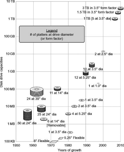
Figure 4.1 Development of spinning disk—based media since 1956.
Storing Bits on Drums
The first method for the storage of bits used magnetic patterns that were deposited on cylindrical drums. The bits were then recovered by a device that would later become the magnetic head. Firstgeneration hard disk drives had their recording heads physically contacting the surface, which severely limited the life of the disk drive. IBM engineers later developed a mechanism that floated the head above the magnetic surface on a cushion of air, a fundamental principle that would become the major piece of physical technology for magnetic disk recording for decades to come.
First Commercial HDD
The first commercially manufactured hard disk drive was introduced on September 13, 1956, as the IBM 305 RAMAC, which was the acronym for “Random Access Method of Accounting and Control.” With a storage capacity of 5 million characters, it required fifty 24-in.-diameter disks, with an areal density of 2 Kbits per square inch (drives today have specs in the hundreds of gigabits per square inch). The transfer rate of the first drive was only 8.8 Kbits/second.
The IBM model 355-2 single-head drive, at that time, cost $74,800, which is equivalent to $6233/Mbyte. Once developed, the IBM engineers determined that a need for removable storage was required. IBM assigned David I. Noble a job to design a cheap and simple device to load operating code into large computers. Using the typical terminology of that era, IBM called it the initial control program load, and it was supposed to cost only $5 and have a capacity of 256 Kbits.
During 1968, Noble experimented with tape cartridges, RCA 45 RPM records, dictating belts, and a magnetic disk with grooves developed by Telefunken. He finally created his own solution, which was later known as the floppy disk. At the time, they called it the “Minnow.” As the first floppy, the Minnow was a plastic disk 8 in. in diameter, 1.5 mm thick, coated on one side with iron oxide, attached to a foam pad, and designed to rotate on a turntable driven by an idler wheel. The disk had a capacity of 81.6 Kbytes. A read-only magnetic head was moved over the disk by solenoids that read data from tracks prerecorded on the disk at a density of 1100 bits per inch.
The first “floppy” disk was hard sectored, that is, the disk was punched with eight holes around the center marking the beginning of the data sectors. By February 1969, the floppy disk was coated on both sides and had doubled in thickness to a plastic base of 3 mm. In June 1969, the Minnow was added to the IBM System 370 and used by other IBM divisions. In 1970, the name was changed to Igar, and in 1971, it became the 360 RPM model 33FD, the first commercial 8-in. floppy disk. With an access time of 50 ms, the 33FD was later dubbed the Type 1 diskette. Its eight hard sector holes were later replaced by a single index hole, making it the first soft sector diskette. The Type 1 floppy disk would contain 77 tracks and the format for indexing of the drive data was referred to as IBM sectoring.
A double-density, frequency-modulated 1200-Kbit model 53FD floppy, introduced in 1976, followed the previous 43FD dual-head disk drive, which permitted read and write capability on both sides of the diskette. Coincidentally, the floppy disk emerged from IBM at the same time the microprocessor emerged from Intel. Disk-based recording technology had actually arrived some 20–25 years prior to the August 1981 debut of IBM’s first personal computer, the PC.
Hard Disk Contrast
By contrast in 1962, IBM had introduced its model 1301, the first commercially available 28 MB disk drive with air-bearing flying heads. The 1301’s heads rode above the surface at 250 microinches, a decrease from the previous spacing of 800 microinches. A removable disk pack came into production in 1965 and remained popular through the mid-1970s. A year later, ferrite core heads became available in IBM’s model 2314, to be followed by the first personal computers (PCs).
The IBM Winchester drive, introduced in 1973, bore the internal project name of the 30–30 Winchester rifle and used the first sealed internal mechanics. The IBM model 3340 Winchester drive had both a removable and a permanent spindle version, each with a capacity of 30 Mbytes. The height of the drive’s flying head had now been reduced from its original 800 microinches to 17 microinches.
Seagate would introduce its 5.25-in. form factor ST-506 in 1980, the drive featuring four heads and a 5-Mbyte capacity.
Personal Computing
IBM introduced the PC/XT, which would use a 10-Mbyte model ST-412 drive. This model would set the standard for the PC-compatible future. A few years later, the 3.5-in. form factor RO352, introduced in 1983 by Rodime, would become and remain the universal size for modern hard disk drives through the early development of modern personal computers until the 2.5-in. was introduced for portable applications in 1988.
Drive Components
The internal components of a typical Integrated Drive Electronics (IDE) magnetic hard disk drive are shown schematically in Fig. 4.2.
Hard Drive Components
The hard disk storage device has been called a Direct Access Storage Device (DASD) or disk. Physically, and internally, the drive consists of one or more magnetic disks mounted to a single central spindle. Traditionally, moving head disks, also called spinning disks, use this center spindle, which is somewhat like an axle, to attach a series of disk platters. As the spindle rotates, the platters are also caused to spin. Platters are often double sided allowing data to be stored and retrieved from each side of each platter.
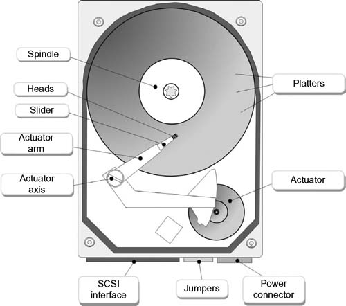
Figure 4.2 Internal components of a hard disk drive.
A boom or moveable arm, called an actuator arm, has a series of read—write heads attached to it—one for each platter. The head is attached to the tip of the boom arm. As the boom arm moves from the outer edge to the inner spindle side of the platter, it can align itself over the tracks on each platter.
Commands given from the disk controller, which reacts to requests from the host device (e.g., a computer), cause the actuator and boom arm assembly to move to a position that allows the drive to read or write data from or to the disk.
Disk drives are inherently mechanical devices, as such they impose certain physical and electromechanical obstacles to achieving perfect performance. One of these obstacles is the time it requires to obtain data once a request to obtain the data is received by the hard drive controller from the host computing device.

Figure 4.3 Layout of the surface of a disk drive, its regions (clusters, sectors, and tracks), and the components of one sector (header, data, and trailer).
The platter surface is divided into regions: tracks, track sectors, geometrical sectors, and clusters. Figure 4.3 shows how these regions are laid out, and the details of the sector consisting of a header (containing synchronization information), the data area, and a trailer (containing the error correction code [ECC] for each data sector).
Rotational Access Time
The surface of the platter has tracks, which are circular concentric rings of data that will cover one complete revolution of the disk’s platter. The cylinder of a disk is that set of the same concentric tracks located on all the disk platters, usually on the top and the bottom of each. Access time, a limiting parameter of the tracks, is a major concern of rotational disks, burdened by the sum of these electrical and mechanical time constraints:
1.Rotational delay (latency)—the time taken by the platter to rotate to the proper location where the data is to be read from or written to
2.Seek time—the time taken by the boom arm with the heads attached to move to the proper cylinder
3.Transmission time—the time taken to read and/or write the data from and/or to the drive platter surface
When compared to a processor’s speed or the time to access solid state memory, disk access time is exceedingly slow. This makes the disk drive the single-most time-restrictive device in a system.
Spinning Platters
The “Winchester” disk drive, well-known over a few decades, consists of magnetically coated platters made from a nonmagnetic material, usually aluminum alloy or glass, which are coated with a thin layer of magnetic material, typically 10–20 nm in thickness. An outer layer of carbon is added for protection. Older disks used iron oxide as the magnetic material, but current disks use a cobalt-based alloy.
The magnetic surfaces of the platters are divided into multiple submicrometer-sized magnetic regions. In each of these areas, a single binary unit of information is contained. Originally, each of the magnetic regions is horizontally oriented, but after 2005, the orientation was changed to be perpendicular for reasons discussed later.
Each of these magnetic regions is composed of a few hundred magnetic grains, arranged in a polycrystalline structure and typically about 10 nm in dimension (10 times less than the thickness of a very thin coat of paint). Each group of these grains are formed into a single magnetic domain. Each group of magnetic regions then form a magnetic dipole. The dipole creates a nearby, highly localized magnetic field, which the pickup heads of the drive use to determine the status of the data in that region.
Attached to the end of each actuator arm is a write head that when precisely positioned over the top of the region can magnetize that region by generating an extremely focused, strong magnetic field. Initially, disk drives used an electromagnet both to magnetize the region and then to read its magnetic field by electromagnetic induction. More recent versions of inductive heads would include “metal in gap” (MIG) heads and thin film (TF) heads, also called thin film inductive (TFI). TF heads are made through a photolithographic process that is similar to the fabrication process of silicon-based microprocessors. The TF/TFI manufacturing process uses the same technique to make modern thin film platter media, which bears the same name.
The evolution of disk drives brought with it increases in data density. The technology eventually found read heads that were made based on the principles of magnetoresistance (MR) ferromagnetics. In MR heads, the electrical resistance of the head changes according to the magnetic strength obtained from the platter. Later developments made use of spintronics, known also as spin electronics and magnetoelectronics. This technology, which is also used to make magnetic semiconductors, exploits the intrinsic spin of the electron and its associated magnetic moment, in concert with its fundamental electronic charge. The magnetoresistive effect in the MR head is much greater than in earlier forms. More about MR and its relative, giant magnetoresistance (GMR) is covered later in this chapter.
The areal density now present in drives that reach multipleterabyte proportions have overcome some incredible complications in magnetic science and physics. As these drives continue to develop, effects where the small size of the magnetic regions create risks that their magnetic state could be changed due to thermal effects have had to be addressed and engineered for. One of the countermeasures to this impending effect is mitigated by having the platters coated with two parallel magnetic layers. The layers are separated by a 3-atom-thick layer of a nonmagnetic rare element, ruthenium (Ru). The two layers are magnetized in opposite orientations, which reinforces each other. A process called “ruthenium chemical vapor deposition” (CVD) is used to create thin films of pure ruthenium on substrates whose properties can be used for the giant magnetoresistive read (GMR) elements in disk drives, among other microelectronic chip manufacturing processes.
Additional technology used to overcome thermal effects, as well as greater recording densities, takes its name from how the magnetic grains are oriented on the platter surface. The technology, called perpendicular magnetic recording (PM), was first proved advantageous in 1976, and applied commercially in 2005. Within only a couple more years, the PMR technology was being used in many hard disk drives and continues to be used today.
Spin Control
Drives are characteristically classified by the number of revolutions per minute (RPM) of their platters, with common numbers being from 5,400 up to 15,000. The spindle is driven by an electric motor that spins the platters at a constant speed.
In today’s disk drives, the read—write head elements are separate, but in proximity to each other. The heads are mounted on a block called a slider, which is set at the end point of a boom arm, or actuator arm, which is positioned by a step-like motor. The read element is typically magnetoresistive while the write element is typically thin-film inductive. A printed circuit board receives commands from the disk drive’s controller software, which is managed by the host operating system and the basic input—output system. A head actuator mechanism pushes and pulls the boom arm containing the read—write head assemblies across the platters. The heads do not actually contact the platters but “fly” over the surface on a cushion of air generated by the air turbulence surrounding the spinning disk platters.
The distance between the heads and the platter surface are tens of nanometers, which is as much as 5000 times smaller than the diameter of a human hair.
Writing and Reading the Disk
The write process of recording data to a hard disk drive happens by directionally magnetizing ferromagnetic material deposited on the surface of the drive platter to represent either a binary 0 or a binary 1 digit. The data is read back by detecting the magnetization of the material when a pickup device (a head) is passed over the top of the tracks where that data is stored.
Disk Drive Form Factors
Disk drives are characterized into groups of “form factors,” which are represented by dimensions, usually expressed in inches. Some believe these numbers relate to the diameters of the physical spinning media (the platters) but in actuality they are rooted in the size of the bay (or slot) that they originally were placed into during the early years of disk drive growth for the PC workstation.
8-in. Form Factor Floppy
The 8-in. format, which started with flexible media around 1971, a decade before the PC, set the stage for the form factor sizing that has sustained the terminology till at least the proliferation of the laptop. The 8-in. drives, introduced by IBM (1972) and DEC, included both single-sided single-density (SSSD) and double-sided double-density (DSDD) versions. The marketed capacities ranged from 1.5 Mbits to 6.2 Mbits unformatted. In these early days, formatting consumed much of the available actual bit storage.
The 8-in floppy could be found in broadcast equipment (e.g., the Quantel PaintBox and others) and continued in use through the 1980s. The last production versions released by IBM (model 53FD) and Shugart (model 850) were introduced in 1977.
5.25-in. Form Factor
The 5.25-in. form factor is the oldest of the drives used in the personal computer world, and it debuted first on the original IBM PC/XT. In the early 1980s, this form factor had been used for most of the IBM PC’s life span but is now most definitely obsolete. The root of the form factor was that it was slotted into the 5.25-in.-wide drive bay that was used first to house the 5.25-in. floppy disk drives found in PCs. The bay size designation has sustained through existing modern PCs and workstations but are now primarily for CD-ROM or DVD/Blu-ray drives or similar devices.
The 5.25-in. hard drive has not been in production for these applications since the late-1980s, although high end drives used in servers were still available through sometime in the mid-1990s. The 5.25-in. form factor was essentially replaced by the 3.5-in. form factor for both physical space reasons and performance improvements.
Internal Components
Generally, the 5.25-in. drives used 5.12-in.-diameter platters. The exterior dimensions are 5.75 in. wide by 8.0 in. deep. The drives were available in only two different height profiles: a full-height version that was the same height as the floppy drive on the original PC and half-height. Other nonstandard heights for 5.25-in. drives were typically 1 in. high or less. Quantum would dub these drives as “low profile” or “ultra-low-profile.” Table 4.1 shows the specifications used in the 5.25-in. form factor family.
Table 4.1
Profiles and Dimensions of the
5.25-in. Form Factor Hard Drives
Bay/Housing Dimensions
| Form Factor | Width (in.) | Depth (in.) | Height (in.) | Life Cycle/Applications |
| 5.25” Full-height | 5.75 | 8.0 | 3.25 | Drives of the 1980s, large- capacity drives with multiple platters through the mid-1990s |
| 5.25” Half-height | 5.75 | 8.0 | 1.63 | Early 1980s through early 1990s |
| 5.25” Low-profile | 5.75 | 8.0 | 1.0 | Middle to late 1990s |
| 5.25” Ultra-low-profile | 5.75 | 8.0 | 0.75–0.80 | Middle to late 1990s |
3.5-in. Form Factor
For over a decade, the 3.5-in. form factor has maintained its place as “the standard” in the desktop PC world although many other high-capacity storage implementations also use this in their multidrive arrays and storage product lines. Like the earlier 5.25-in. form factor, the 3.5-in. form factor is named not for the dimensions of the drive components themselves but rather for the way they fit into the same footprint of the drive bay originally created for the 3.5-in. floppy disk drives.
A 3.5-in. form factor drive will traditionally use 3.74-in. platters with an overall housing width of 4.0 in. and depth of approximately 5.75-in.
Higher speed 10,000 RPM spindle speed drives reduced their platter size to 3 in., with 15,000 RPM (Seagate) drives using 2.5-in. diameter platters. The 3.5-in. form factor has been maintained for compatibility, but the reduction in size of the physical media is for performance purposes.
3.5-in. Profiles
The 3.5-in. form factor drives come in the two profiles shown in Table 4.2. The larger profile half-height drive, which is 1.63 in. in height, uses this name because the drives are of the same height as the older half-height 5.25-in. form factor drives. Half-height 3.5-in. form factor drives may still be found in servers and other higher end storage systems.
The “slimline” or “low-profile” drive found in the 3.5-in. form factor family is only 1 in. in height. Some drives have reduced their height from the 1-in. standard and are now available in 0.75-in. high versions.
Table 4.2
Profiles and Dimensions of the
3.5-in. Form Factor Hard Drives
Bay/Housing Dimensions
| Form Factor | Width (in.) | Depth (in.) | Height (in.) | Life Cycle/Applications |
| 3.5” Half-height | 4.0 | 5.75 | 1.63 | High-end, high-capacity drives |
| 5.25” Low-profile | 4.9 | 5.75 | 1.0 | Common to most PC drives, industry recognized standard |
Table 4.3 Profiles and Dimensions of the 3.5-in. Form Factor Hard Drives
Bay/Housing Dimensions
| Form Factor | Width (in.) | Depth (in.) | Height (in.) | Life Cycle/Applications |
| 2.5”/19 mm height | 2.75 | 3.94 | 0.75 | High-capacity drives used in larger laptops |
| 2.5”/17 mm height | 2.75 | 3.94 | 0.67 | Midrange capacity drives, used in some laptops |
| 2.5”/12.5 mm height | 2.75 | 3.94 | 0.49 | Low capacity drives, used in smaller laptops (and in some notebooks) |
| 2.5”/9.5 mm height | 2.75 | 3.94 | 0.37 | Low-capacity drives used in mobility platforms, very small laptops, mininotebooks/notebooks |
2.5-in. Form Factor Drives
The introduction of 2.5-in. form factor drives made notebook computers much more popular, with mobility being the driving factor. Many laptop or notebook computers have used 2.5-in. form factor hard drives (or less) for the following reasons:
- Size reduction—the drives take up less space, allowing laptops and notebooks to be reduced in overall size.
- Power reduction—the smaller drives consume less power and in turn extend battery life.
- Rigidity and durability—smaller platters reduce the susceptibility to shock damage.
Other Form Factors
The first 1.8-in. form factor drives were introduced in 1991. Integral Peripherals’ 1820 model was the first hard disk with 1.8-in. platters. After the introduction of this model, and the 2.5-in. form factor drives, the previous “mold” for designating drive form factors was broken. The newer technologies would not be used as much in bays or slots but were now being placed into sleds, holders, or as PC Card disk drives.
The first 1.3-in. form factor was introduced in 1992 by Hewlett-Packard as the model C3013A. The drive capacities reached in the 30–40 Gbytes domain during early 2008.
Disk Performance Optimization
To maximize disk drive performance, many elements must work together to achieve the highest efficiencies. Such elements include the optimization of the mechanical systems, best use of the available bandwidth, management of the number of devices being accessed on the bus, and the application of best approach algorithms taking into account the usage and purpose that the disk drives will be deployed in.
To mitigate problems with delays, requests for data read and writes must be serviced in a logical order based on several factors. Some of these are mechanically dependent and others algorithm dependent. To optimize disk drive performance, service requests should be administered with the least amount of mechanical motion.
Latency
Any delay in getting a command started or the overall time involved between issuing a command and having it (fully) executed is considered latency. Latency can be impacted by several factors, which will be discussed in the following sections.
Bandwidth
A disk’s bandwidth is defined as the total number of bytes transferred, then divided by the total time between the first request for service and the completion of the last transfer. Controlling the bandwidth allocation requires scheduling of requests for service.
Disk Scheduling
In the early years of disk drive development, disk scheduling algorithms concentrated mostly on minimizing the seek time, that is, the time from when the host request is issued to when the request is fulfilled. The majority of the time required to fulfill a request involves positioning the head over the data track itself. This includes getting the actuator arm that carries the heads to the proper position ahead of when the track actually appears beneath the head and without having to wait another rotational period for the track to realign under the head. The length of time these actions take becomes the single highest contribution to disk access latency.
With the continuous development of disk drives came an abundance of improvements in rotational optimization that included the control of when the various read-write requests were actually executed, along with variations in the algorithms that make up how the disk performs. Such improvements were covered under a set of terminologies and types of actions referred to as "scheduling."
First-Come First-Served Scheduling
This mode is almost primitive given the changes in drive technologies over the past two decades. As the name suggests, the first-come first-served (FCFS) mode acts on the first instruction it receives and completes it before accepting the next one. This form of scheduling, also known as “first-in first-out” (FIFO) in some circles, results in significant wait times for the head or arm assembly to get from any one location to another. Moreover, under heavy request loads, the system can be inundated to the point it can lose track of the processing order.
This unregulated scheduling mode has at least one major consequence. Principally, FCFS has the potential for extremely low system throughput, typically resulting in a random seek pattern caused by the controller’s inability to organize requests. This disorganization induces serious service delays.
FCFS has some advantages. First, the access time for the servicing of requests is fair. FCFS prevents the indefinite postponement of requests for services, something other scheduling modes have to their disadvantage. Second, there is low overhead in the execution time for service requests, that is, no additional processing is considered. This is essentially “brute force” action at its highest.
Shortest Seek Time First Scheduling
This scheduling mode, as its name implies, uses the shortest seek time first (SSTF) concept to recognize where the head and actuator assembly is related to the particular cylinder it is positioned over, then ties that position to the execution of the next request.
SSTF is a direct improvement over the FCFS algorithm. It works by a process whereby the hard drive maintains an incoming buffer to hold its continually changing set of requests. A cylinder number is associated with each incoming request. A lower cylinder number indicates that the cylinder is closer to the spindle. A higher number indicates that the cylinder is further away, that is, closer to the edge of the disk platter. Of course, the rotational speed is greater at the edge, and the distance that point at the edge must travel to complete a full rotation is much farther than near the spindle center. There is more data on the outer edge and thus more places to locate at the same amount of time.
Because this variance cannot be substantiated and depending on how the numbers are generated, most specifications will average the number from each end of the platter or use statistics that come from the middle part of the disk as their reference point.
The SSTF algorithm resolves which request is nearest to the current head position, and then it places that request next in its queue. Compared with FCFS, SSTF results in a higher level of throughput, with lower response time, and produces a sensible solution for batch processing on a system-wide basis.
The SSTF disadvantages stem from unfair access times in the servicing of requests. Activities are now dependent on the previous data access. Situations where the data is more randomly scattered about the drive increases the access time latency. Contiguously laid down sequential data, such as in the recording or playout of a lengthy video segment, will not see an increase in access times. However, randomly distributed data laid down inconsistently during the write process, and then randomly recalled by a different application, may see extensive increases in the access time.
The SSTF also creates the possibility for an indefinite postponement of requests for services. If all the data reading activities were near the same region that the heads were currently positioned in, a potentially lengthy period could result before data located in another region of the platters might be accessed. SSTF produces a high variance in overall response times, which is generally seen as unacceptable for interactive systems.
Access Time Components
Access time is the greatest contributor to the high side of the latency equation. The time that it takes to access data on a drive is impacted by two major components, both mechanical in nature.
Rotational Delays
Rotational delay (or latency) is the additional time required for the spindle to rotate to the desired sector of a cylinder such that the appropriate data is positioned below the read—write head itself. When the rotational speed is faster, as expressed in revolutions per minute (RPM), there is less rotational delay because the period required to reach that position is shorter.
Delay is further affected by the number of cylinders and whether those cylinders are at the edge (i.e., a greater distance to rotate for positioning) as opposed to near the spindle (thus, a lesser distance to rotate for positioning).
Seek Time
This is the time required for the disk to move the heads to the cylinder containing the desired sector, that is, the time required for the head and actuator arm to move from its previous (or current) position to its next position such that it is ready to actually perform the requested read or write function.
Seek time can have a bigger impact on the overall latency than the rotational delay. This is why disk optimization and scheduling algorithms concentrate more on reducing seek times.
Servicing and Scheduling Criteria
The policies used in the processes associated with servicing and scheduling requests for access (both read and write) are categorized according to certain criteria.
- Throughput—the volume of data accessed and that is actually retrieved from the disk or written to the disk, in a given time period.
- Mean response time—the sum of the wait time and the service time in accessing the data.
- Predictability—calculated as the variance of response times as a standard deviation from a mean. If the variance from the mean is high, there is less predictability. If the variance from the mean is low, there is more predictability.
Whenever a policy can keep these variances low, there will be a tendency to stabilize the servicing of those requests. How those optimizations are fulfilled is the job of the microcode that is written into the drive’s controller. There are proven strategies used in optimizing seek times, which are discussed in the next section.
Optimization Strategies for Seek Times
Improvements that have been made from the previous FCFS and SSFT algorithms include SCAN and C-SCAN. Each of these descriptions are much deeper looks under the hood than the general user would probably need to know, but these approaches show how disk drive technologies have been combined to provide us all with greater capabilities than back in the days of floppies and 5.25-in. hard drives.
SCAN
One advancement over SSFT is called SCAN. To minimize seek time, the disk controller code will first serve all its requests in one direction until there are no more in that direction. Then, the head movement is reversed, and the service is continued. SCAN enables a better servicing of requests and, in turn, provides a very good seek time because the edge tracks will receive better service times. However, one should note that the middle tracks will get even better service than the edge tracks.
When the head movement is reversed, the drive will first service those tracks that have recently been serviced, where the heaviest density of requests, assuming a uniform distribution, are presumed to be at the other end of the disk. The SCAN algorithms will utilize principles that consider directional preferences and then service newly arriving requests only if they are ahead of the direction of the current SCAN.
The direction of the head/actuator assembly is called a sweep. The sweep generally continues from the spindle toward the outermost track until the targeted track is reached or until there are no further requests in that particular direction. Once the target or the edge is reached, the direction is reversed until the sweep reaches the innermost track or again, until there are no more requests in that direction.
Elevator Algorithm
In order to optimize efficiency, the sectors on a hard drive and the requests for data access should not be based on the order in which requests were received. The action order should be set by where the current head position of the drive is at the instance the request is received. Since a hard drive will continually receive new requests, each of them is placed into a queuing system whose operational requirement is to fulfill the current requests and then remove the older requests. Sometimes these requests are delayed, especially since the queuing system will continually re-order those requests based on specific controller algorithms and the physical functionality of the drive.
The SCAN algorithm acts like and is sometimes referred to as “elevator seeking” because it is constantly scanning the disk using the motion of the disk’s actuator arm and the head positioning associated with that arm to determine which requests it should act on. The “elevator algorithm” is essentially a scheduling routine that, in principle, works like a building elevator: it moves only in the direction of a request from passengers and stops only on the floor that people wish to get on or off.
When a drive is idle and a new request arrives, the initial head and actuator assembly movement will be either inward or outward in the direction of the cylinder where the data is stored. Additional requests will be received into the queue, but only those requests in the current direction of arm movement will be serviced until the actuator arm reaches the edge or the center spindle side of the disk, depending on the direction it was travelling at that time. This is just like the SCAN principle described previously.
SCAN Variations
SCAN has developed into subsets that use other algorithms that are specific to the drive and controller microcode instructions written into firmware. Each of these variations offers differing tactics to handle the servicing of requests. Some of the following SCAN alternatives may still be found in various hard drive applications.
C-SCAN
This variation, also known as the Circular Elevator Algorithm, provides a more uniform wait time than the straightforward SCAN methodology. C-SCAN ensures that a scheduling request for service will only occur in a single direction, treating the cylinders as a circular list that wraps around from the last cylinder to the first cylinder.
In C-SCAN mode, the head and actuator arm assembly travels from one side of the disk to the opposite side using a “shortest seek mode” for the next request in the queue. The seek direction begins at the center (spindle side) and advances outward to the edge. Once the arm reaches the edge of the disk, it then rapidly returns to the spindle side of the disk and continues servicing the queued requests in a single direction. The arm essentially only scans in a “center to edge” only direction, and then retraces (like analog television CRT raster scanning) back to the center. C-SCAN optimizes performance by ensuring that the expected distance from the head to the next data sector is always less than half the maximum distance that the arm must travel.
FSCAN
Another alternative disk scheduling algorithm is called FSCAN. This mode uses two subqueues. As the scan is in process, all the current requests are placed in the first queue and all new (incoming) requests are placed into the second queue. The servicing of any new requests, stored in the second queue, is deferred until all current (i.e., “old”) requests have been processed. Once the current scan is completed, which may take several passes from center to edge, all the first-queue requests are flushed, the arm is taken to the new queue entries, and the process is resumed all over again.
LOOK
This mode is similar to SCAN, with a twist. Instead of continuing the sweep to one side and returning, the head and actuator arm assembly will stop moving in its current direction, either inwards or outwards, when there are no further requests that reside in that particular direction.
C-LOOK
A version of C-SCAN, this C-LOOK mode has the head and actuator arm assembly tracking only from the first to the last request in one of the directions. The actuator arm then reverses direction immediately and without tracking the disk fully again from the first to the last.
N-Step-SCAN
With SSTF, SCAN, and C-SCAN, there is the possibility that the arm may not move for a considerable period of time. This probability is more evident in high-density disks that are likely to be affected the most. Low-density disks and/or disks with only one or two surfaces are likely candidates for N-Step-SCAN, also known as N-Step LOOK. The primary feature of this mode is aimed at avoiding “arm stickiness.”
N-Step-SCAN uses directional preferences and a disk scheduling algorithm that segments the request queue into subqueues of length N. Breaking the queue into segments of N requests makes service guarantees possible. Subqueues are processed one at a time. While a queue is being processed, new requests must be added to some other queue. If fewer than N requests are available at the end of a scan, then all of them are processed with the next scan.
When the values of N are large, the performance of N-step- SCAN approaches that of SCAN. When the value of N equals 1, then a FIFO policy is adopted. N-Step-SCAN works like SCAN, except that after a directional sweep has commenced, any newly arriving requests are then queued for the next sweep. Therefore, this algorithm will service only N requests at a time. Subsequent requests entering the request queue will not get pushed into N-sized subqueues, which are already full per the “elevator algorithm.” Thus, request starvation is eliminated, and guarantees of service within N requests is made possible.
The N-Step-SCAN mode provides for good overall throughput. Of all the modes discussed earlier, it has the lowest variances because it works by reordering the service request queue for optimum performance and throughput.
EDF
Earliest Deadline First, or EDF strategy, is a mode where the block of the stream with the nearest deadline would be read first. EDF is utilized when there is a real-time guarantee requirement for the data access, as in streaming video.
EDF in its precise sense results in poor throughput and excessive seek time. EDF is most often applied as a preemptive scheduling scheme. The cost penalties for preemption of a task and scheduling of another task are considerably high. The overhead caused by task preemption is on the same order of magnitude as the time incurred for at least one disk seek. Thus, EDF needs to be adapted or combined with file-system strategies.
You may also see EDF augmented with the JIT designation, as in EDF/JIT, referring to the extension “just in time.”
SCAN-EDF
This strategy combines both SCAN and EDF methods using the seek optimization benefits of SCAN and the real-time guarantees of EDF. Like in EDF, the service request with the earliest deadline is always served first, among those requests with the same deadline. The request that is first, according to the scan direction, is served first. Among the remaining requests, this mode is repeated until there are no requests with this deadline left.
The hybrid SCAN-EDF variation of the SCAN disk scheduling access algorithm is intended for use in a real-time environment where, in general, the requests are served according to an “Earliest Deadline First” (EDF) mode. When two requests share the same deadline, they may be reorganized according to SCAN.
An appropriate example of how to apply SCAN-EDF is when a videoserver retrieves file data from a hard disk during the playout function. In this process, video that streams from a system will impose tight real-time constraints on data delivery from the storage system. One cannot simply “wait” for the actions of the disk scheduling to preempt a file being read. In a simpler sense, if a videoserver retrieves data once every second for each video channel, then SCAN-EDF can be applied and the goal of reducing the effects of seek overhead can be better met.
Deadline Sensitive SCAN
Usually written as “DS-SCAN,” Deadline Sensitive SCAN is an algorithm for the scheduling of real-time disk I/O requests. DS-SCAN is a simple, yet powerful hybrid of traditional EDF and SCAN algorithms. Fundamentally, the feature of DS-SCAN is that it closely imitates the behavior of the SCAN algorithm so as to increase the effective throughput of disk, but subject to the deadlines of realtime request constraints so that the services are not missed.
Functionally this algorithm attempts to schedule the disk servicing requests (i.e., the “I/O requests”) without impacting the deadlines of the real-time requests. Traditional SCAN does not take this into account. DS-SCAN does not have a fixed service schedule, which provides it with the flexibility to deal with realtime request streams that prescribe finely tuned deadlines. Its framework allows for the support of periodic real-time, aperiodic real-time, and best-effort requests, in whole or as a mixed set.
DS-SCAN will dynamically track how tight the request deadlines are using the idea of reserving “spare deadlines” that can be implemented when they are in demand. This concept basically follows the SCAN order until it needs to defend the real-time requests, during which time it shifts to EDF order.
Best Effort
This classification, one of two types in DS-SCAN, has no deadlines associated with it. Best effort requests could be considered against the disk scheduling model when compared with real-time scheduling. This is not to say it is detrimental to the DS-SCAN model; it might be considered as a relaxation mode, when the disk request algorithm can do what it is best suited to do given the previous mode it was in.
Real-Time Disk Scheduling
Virtually all disk devices will utilize an intelligent disk scheduling algorithm that incorporates “positional awareness.” Many disks themselves may have more intelligence and efficient scheduling capabilities than those found in external schedulers. Today’s storage systems may find many, sometimes varying, instances of disk scheduling methodologies present in multiple locations of the hardware, such as in the disk itself or in the RAID controller.
With today’s emphasis on real-time content delivery, a real-time disk scheduling algorithm is essential. However, the bar must be raised when there are continual and concurrent requests to provide service access from multiple sources. This kind of activity is referred to as “concurrent access requests.” It is becoming more important to address these issues as single drives are now exceeding 2 Tbytes and will approach the domain of 5 Tbytes or so before too long.
To address these growing activities in concurrent access requests, researchers have been exploring ways to maximize the throughput for modern storage devices by allowing concurrent I/O requests at the device whenever possible. Real-time disk scheduling algorithms of the past were modeled around a storage device receiving a single request at a time. This model dramatically reduced utilization and slowed the throughput in modern storage devices.
Today, RAID arrays and most disks already have an efficient positional-awareness scheduling algorithm built into firmware or software controllers. The controls are optimized for the proficiencies of the drive and per the kinds of activities requested through the host in concert with the file system. DS-SCAN is utilized as needed, but it can suffer from conditions where multiple requests arrive at the same time.
The DS-SCAN algorithm can be extended so as to properly account for multiple outstanding service requests and in turn guarantee those real-time constraints for both outstanding and pending real-time requests. The name that is associated with the research and proposals from HP Labs is “Concurrent DS SCAN” (CDS SCAN). For a more detailed look at the research proposal from HP Labs please refer to the “Further Readings” section at the conclusion of this chapter.
Group Sweeping Scheduling
Group Sweeping Scheduling (GSS) is aimed at reducing the number of disk actuator arm movements thus reducing access time and latency. In this model, requests for services are served in cycles (i.e., a “round-robin- like” manner), with the set of N streams being divided into G groups. These groups are then served in a fixed order.
The individual streams within a group are served according to SCAN, that is, there will not be a fixed time or order by which the individual streams within a group are served. In other words, in one cycle, a specific stream may be the first to be served and then in another cycle it may be the last.
A variable smoothing buffer, sized according to the cycle time and data rate of the stream, is used to assure continuity. If the SCAN scheduling strategy is applied to all streams of a cycle without any grouping, the playout of a stream cannot be started until the end of the cycle of its first retrieval where all requests are served once because the next service may be in the last slot of the following cycle. As the data must be buffered in GSS, the playout can be started at the end of the group in which the first retrieval takes place. As SCAN requires buffers for all streams, in GSS, the buffer can be reused for each group. Further optimizations of this scheme are proposed.
In this method, each stream is served once in each cycle. GSS is a trade-off between the optimization of buffer space and arm movements. To provide the requested guarantees for continuous media data, a “joint deadline” mechanism is introduced whereby each group of streams is assigned one deadline, that is, the joint deadline. This deadline is specified as being the earliest one out of the deadlines of all streams in the respective group. Streams are grouped such that all within the group are comprised of similar deadlines.
Capacity Factors, Transfer Time and Obstacles
Besides the various algorithms and mechanical controls, disk drives are generally specified according to their storage capacity. The factors affecting storage capacity include areal density, track density and recording density. These, along with transfer time impacts and other obstacles impacting hard drive performance are discussed in the next sections.
Areal Density
The volume of data capable of being stored in a given amount of hard disk platter space is called the “areal density” of that specific disk drive. Over the years, areal density has been equated, improperly, to bit density or sometimes just “density.” In actuality, areal density is a two-dimensional metric calculated by multiplying two linear measures: recording density (bit density) and track density. The result is measured in bits per square inch (BPSI or bits/in.2).
Track Density
This is the measure of how tightly the concentric tracks on the disk are packed. That is, the number of tracks that can be placed down per inch of radius on the platters. If there is a usable storage space along a radius equal to 1.0 in. of length, and in that amount of space the hard disk has 20,000 tracks, then the track density of that drive would be approximately 20,000 tracks per inch (TPI).
Linear or Recording Density
The linear or recording density is defined as the measure of how tightly the bits are packed per unit length of track. If a 1-in. track can hold 225,000 bits of information, then the linear density for that track is 225 kbits per inch per track (BPI).
Nonuniformity
The tracks are concentric circles, so every track on the platter’s surface will be of different length. Not every track can be written with the same density. So, the numbers are rather nebulous, and you will find that manufacturers usually quote the maximum usable linear record density capacity for each drive.
Densities on modern drives can be in the upwards of billions of bits per square inch. The usual metric is expressed as “gigabits per square inch” (Gbits/in.2). The product of the track density and linear or record density yields the areal density of the drive. You will find that in some cases, the two measures that encompass areal density are specified separately. You will further note that there will be data sheets that do not show the two components individually. Thus, the expression is difficult to evaluate and leads engineers into looking at each of the numbers separately, especially since they are quite different in terms of how they reflect the aspects of disk drive performance.
Transfer Time
Transfer time is another variable that is associated with disk drive specifications. This metric ties together rotational speed, the number of bytes to be transferred, and the seek time.
Transfer time is directly linked to access time. Access time is calculated as a summation of the “command overhead time” (the time from when a command is issued to when the command is fulfilled) plus the “seek time” added to the “settling time” of the head and actuator arm assembly, and then any additional rotational latency or other latencies that are accumulated due to head and platter positioning within the system. Transfer time also includes the number of bytes to be transferred, the number of bytes on a track and the rotation speed of the drive platter assembly.
Obstacles
Areal density is strongly correlated to the transfer rate specifications of the disk drive. In general, the higher the drive’s areal density, the higher its transfer rates will be. Most of the improvements in transfer rate are due not to track density but by the ability to increase bit density.
The main obstacle to increasing track density is assuring that the tracks are not so close that erroneous data would be read. This is exacerbated when the reading of one track causes the heads to pick up data from adjacent tracks. To prevent this anomaly, the magnetic fields are made weaker to prevent interference. This has lead engineers to develop much better designs in read—write head technologies, perpendicular recordings, and the use of Partial Response Maximum Likelihood (PRML) methods to improve signal detection and processing.
Balancing performance with the parameters of bit density and transfer rates creates foggy understanding of what these ratios really mean. For example, if drive “0” has an areal density 5% lower than that of drive “1,” but its bit density is 10% higher, it will have a higher transfer rate than drive “1.” Bit density and track density impact positioning performance. An increase in either one will allow data on the hard disk to be stored physically closer together on the disk. The effect is that it reduces the distance that the read—write heads must seek to find different magnetic segments of data stored on the disk; this slightly improves seek time.
Again, the linear density of a disk is not constant over the drive’s entire surface. Also, remember that when reading density specifications, the cut sheets usually list only the maximum density of the disk.
Current high-end hard disks are exceeding 100 Gbits/in.2 in areal density, and it has been only a few years since 1 Gbits/in.2 was state of the art. For example, in March 2010, Toshiba Corporation announced additions to its 5400 RPM line of 2.5-in. HDDs. One of its features is an areal density of 839.1 Mbits/mm2 (~542 Gbits/ in.2). This is an incredible piece of science, given that as the bit size drops and the bits are packed closer together, the magnetic fields must become weaker. This then requires more sensitive head electronics to properly detect and interpret the data signals. Achieving these increased bit packing densities was possible by developments in head technologies and associated algorithms such as PRML, which are discussed shortly.
Read—Write Heads
Disk drive read—write heads are functionally tiny electromagnets that transform electrical signals to magnetic signals and magnetic signals back into electrical signals. Each bit of data stored on the hard disk is encoded using a special method that translates zeros and ones into patterns of magnetic flux reversals.
Originally, the heads were composed of ferrite, metal-ingap, and thin-film materials, made to work by the use of two main principles of electromagnetic force. The first (write process) applies an electrical current through a coil, which produces a magnetic field. The direction of the magnetic field produced depends on the direction of the current that is flowing through the magnetic coil. The second (read process) is opposite, whereby applying a magnetic field to a coil causes an electrical current to flow, which is detected by the coil and then records the direction of the magnetically charged particles on the disk.
The direction that the current flows depends on the direction of the magnetic field applied to the coil.
Magnetoresistance (MR)
Newer magnetoresistive (MR) heads use a different principle to read the disk. The complete technical name for the first-generation MR heads is anisotropic magnetoresistive (AMR), yet they have traditionally been called just “magnetoresistive.” However, with “giant magnetoresistive” (GMR) heads on the market, there is the possibility for confusion between the terms “magnetoresistive” and “giant magnetoresistive,” so some companies have reverted to calling the older MR heads “AMR” heads to distinguish them from GMR.
An MR head uses a conductive material that changes its resistance in the presence of a magnetic field. As the head flies over the surface of the disk, the head significantly changes the resistance as the magnetic fields change in correspondence to the stored patterns on the disk. A sensor in the assembly detects these resistive changes and the bits on the platter are read.
MR heads have allowed significantly higher areal densities to be used on the platters, increasing the storage capacity and, to a lesser extent, the speed of the disk drive. The MR head is several times more sensitive to magnetic flux changes in the media, which allows the use of weaker written signals, and lets the magnetic bits (grains) be closer spaced without causing interference to each other. This higher packing density, that is, the “areal density,” has contributed significantly to large improvements in overall storage capacities.
Read Only
MR technology is available only for the read process. For the write process, a separate standard thin-film head is used. By splitting the duties between the two types of heads, additional advantages are gained. The traditional ferrite-based heads that did both reading and writing are an exercise in trade-offs. Efficiencies were hard to come by, and balancing those improvements that would make the head read more efficiently would make it write less efficiently. Furthermore, for the best results, a wider data track was written to ensure the media was properly magnetized, but the heads would prefer to read a narrower track to insure signals from adjacent bits were not accidentally picked up.
These dual head combinations are sometimes referred to as “merged heads.”
Giant Magnetoresistance (GMR)
Several years ago (predating its 1997 introduction), IBM introduced the “giant magnetoresistive” (GMR) read head. These heads work on the same fundamental principles as the original anisotropic magnetoresistive (AMR or MR) heads but use a different design that results in better performance.
GMR heads are not named “giant” because of their size; in fact, they are actually smaller than the regular AMR (or MR) heads developed by IBM many years ago. Rather, GMR heads are named after the giant magnetoresistive effect, first discovered in the late 1980s by two European researchers, Peter Gruenberg and Albert Fert, working independently. The researchers found when working with large magnetic fields and thin layers of various magnetic materials, they noticed there were very large resistance changes when these materials were subjected to magnetic fields. Although their experiments used techniques and materials not suitable for manufacturing, the discoveries provided the basis for the GMR technology.
GMR Effect
Engineers and scientists at IBM’s Almaden Research Center developed GMR, turning their discovery into a commercial product after experimenting with many different materials. The GMR effect would work when materials were deposited onto multiple layers of materials through sputtering, which is the same technique used in making thin-film media and thin-film read—write heads.
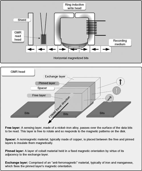
By December 1997, IBM had introduced its first hard disk product using GMR heads, which today are comprised of four layers of thin material sandwiched together into a single structure (as shown in Fig. 4.4).
When the GMR head passes over a magnetic field of one polarity (e.g., “0” on the disk), the free layer has its electrons turn to be aligned with those of the pinned layer. This creates a lower resistance in the entire head structure. When the head passes over a magnetic field of the opposite polarity (“1”), the electrons in the free layer rotate, so they no longer are aligned with those of the pinned layer. This effect increases the resistance of the overall structure, which is caused by changes to the spin characteristics of electrons in the free layer. IBM named these structures “spin valves,” like the rotatable shut-off valve found in a plumbing fixture.
Highly Resistive
GMR heads are superior to conventional MR heads because they are more sensitive. The older MR heads would exhibit a resistance change when passing from one magnetic polarity to another of typically about 2%. In GMR heads, this range is increased to between 5% and 8%. This lets the GMR heads detect much smaller, weaker signals. GMR heads are typically fitted with a shroud to protect against stray magnetic fields that are made much smaller and lighter than MR heads. This makes the GMR heads much less subject to interference and noise due to their increased sensitivity.
Figure 4.4 GMR head construction.
Special amplification circuits convert the weak electrical pulses from the head into digital signals representing the data read from the hard disk. Error detection and correction circuitry compensate for the increased likelihood of errors as the signals get weaker on the hard disk.
Partial Response Maximum Likelihood
Coupled with magnetoresistive (MR) head technology is another principle known as Partial Response Maximum Likelihood (PRML). Together with the read channel technologies, these have become two of the most significant solutions in drive head technologies. Alone, each delivers substantial improvements in certain areas over legacy drive technologies with inductive heads and peak detection read channels. MR and PRML reduce the necessity for many of the capacity and performance trade-offs inherent to disk drive design while continuing to decrease the costs per gigabyte of magnetic spinning disk storage.
PRML Read Channels
PRML read channels further provide another means of obtaining areal density improvements while also aiming to improve performance through increased data transfer rates. As bit densities increase, so do the possibilities of intersymbol interference (ISI). ISI results from the overlap of analog signal “peaks” now streaming through the read—write head at higher rates. ISI has traditionally been combated by encoding the data as a stream of “symbols” as it is written, which separates the peaks during read operations. The problem was that the encoding process requires more than one symbol per bit, which produces a negative impact on both performance and disk capacity.
With PRML, read channels separating the peaks during read operations is unnecessary. Instead, advanced digital filtering techniques are used to manage intersymbol interference. The process uses digital signal processing and “maximum likelihood” data detection to determine the sequence of bits that were “most likely” written on the disk.
Drives using PRML read channels can use a far more efficient coding scheme that obtains its value proposition by its ability to now facilitate the accuracy of the data during read back. For example, drives using traditional peak detection typically experience a ratio of user data to stored symbols of 2–3. Thirdgeneration PRML development for drive manufacturers are now using an encoding scheme that increases that ratio to 16–17. This simple relationship “predicts” 40% more capacity on the disk for actual user data and in turn has a positive impact on the internal data transfer rate for the drive system.
Complementary Advantages
Both these technologies (MR and PRML) are capable of delivering substantial advantages over traditional disk drive technologies. As the development of PRML has increased, inductive head (MR) drives were delivering a 20%–30% increase in areal density for a similar price point to the older technologies. When implemented together, MR heads and PRML read channels provide for faster data transfers, fewer soft errors per unit of storage, and the ability to filter the signal from the disk, which in turn provides a cleaner signal recovery during the read process.
These forms of disk drive head implementations and recording processes have increased areal density by record amounts. Since combining them with the application of the GMR technology, collectively, these types of disk heads been leading the race to better drive performance.
No-ID R ecording
One further discussion about disk drive performance increase relates to the header that is typically recorded at the start of each sector on a disk. Usually, disks will have a prefix portion, or header, that is used to identify the start of the sector. The header contains the sector number and a suffix portion (a trailer or footer), which contains a checksum that is used to ensure the integrity of the data contents. Newer drives are now omitting this header and use a No-ID recording, a process whereby the start and end points of each sector are located via predetermined clock timing. No-ID recording allows more space for actual data.
Yet that is not the end of the advances in creating higher volume and greater densities in recording, as will be seen in the next section.
Advanced Format Sector Technology
This new technology increases the capacity of the hard drive while still maintaining data integrity. Drive manufacturers as early as 2009 have begun to use this new technology as a means to effectively increase the bits stored on the drives. Advanced Format drives have incorporated several changes that seek to optimize the data structure on the hard drive. Fundamentally, the technology increases the physical sector size from the traditional 512 bytes to a more efficient 4096 (4K) byte sector size.
Because this is transitory technology, an inordinate amount of existing drives would be impacted, so as to ease the transition, the current Advanced Format drives will provide “512-byte emulation” (also written 512e) located at the drive interface. The intent of 512e is to maintain backward compatibility with legacy applications.
Impacts to Operating Systems
Most modern operating systems have been designed to work efficiently with Advanced Format (AF) drives. For optimum performance, it is important to ensure that the drive is partitioned correctly and that data is written in 4K blocks by both the operating system and the application. Recent operating systems handle this automatically, and legacy systems would need to be looked at on a case-by-case basis.
Legacy Limitation
Hard drive technology from 30 or more years ago set the basis for most of the “storage constraints” by limiting the amount of user data that could be stored in the traditional 512-byte sectors. The storage industry has sought to improve this stale architecture by changing the size of the sectors on the media so that they can store 4096 bytes (4kbytes) of data per sector as opposed to legacy devices with their 512-byte limit.
Advanced Format drives use larger sectors, now 4K bytes, which is the equivalent of putting the eight legacy (512-byte) sectors into one new single 4K sector. The Advanced Format approach yields two benefits (see Fig. 4.5). First, by eliminating the repetitive portions that would be found if using the legacy 512-byte methodology, the amount of space available for actual data increases in proportion to the removal of the seven extra sets of fields in the logical block. Notice that each legacy 512-byte sector had to include a Sync Field/DAM section and an ECC section, plus a gap. The Advanced Format technology reduces this to just one set for each larger 4K sector.
By optimizing the eight sets of overhead associated with each smaller sector, the drive overall will use less space to store the same amount of information resulting in a format efficiency improvement almost equivalent to one block for every eight.
The second benefit is that the AF uses a larger and more powerful error correction code (ECC), which provides for better integrity of user data. These benefits improve overall system performance by adding capacity and reducing overhead.
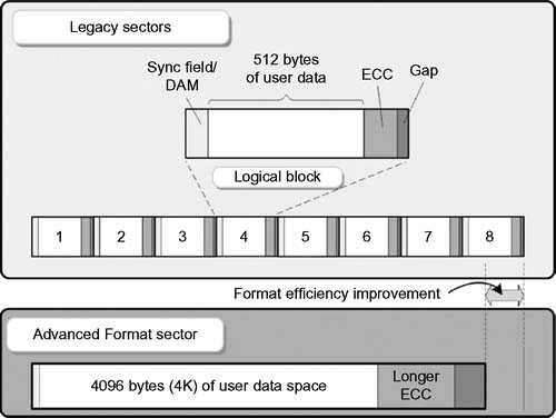
Figure 4.5 Comparison of legacy and Advanced Format sectors.
Reducing Overhead
In the legacy format, each sector of the track contained a gap, a Sync/DAM (lead-in), and error correction information. The current (legacy) architecture is quite inefficient for Error Correction Code (ECC), so there is a significant overhead component required to support multiple blocks of ECC.
Eliminating the extra Sync/DAM blocks, intersector gaps, and the eight individual blocks of ECC improves error rates within the same capacity of storage. It increases data integrity through a more robust error correction scheme that uses a longer set of ECC code words. A 50% increase in burst error correction is obtained when using AF, again through the use of the larger ECC code word.
Compatibility
Increased sector sizes are already employed by many disk drive interface technologies; however, many systems including PCs, digital video recorders, mobile devices, and servers are inflexible and will only work with 512-byte sectors. To retain compatibility with existing devices, Advanced Format media includes an emulation mode, whereby the 512-byte sector device is modeled at the drive interface (see Fig. 4.6).
By mapping logic sectors to physical sectors, compatibility at the interface is maintained.
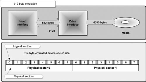
Figure 4.6 Emulation mode for 512-byte hosts uses “512e” to interface Advanced Format media with legacy systems.
Advanced Format Standards
Provisions for the Advanced Format technology are included in the efforts of the American National Standard of Accredited Standards Committee INCITS working group, which drafted the “AT Attachment 8-ATA/ATAPI Command Set (ATA8-ACS)” document in 2007, and in the “SCSI Block Commands (SBC-3)” standards, which allow for a disk drive to report Advanced Format sector sizes and other performance optimization information. These standards are used for SATA, SAS, USB, and IEEE 1394 interface technologies.
The Advanced Format technology is designed to work on most of the current operating systems including Windows Vista, Windows 7, and Mac OS X. It is not optimized for legacy OSs such as Windows XP, but utilities are available that allow Advanced Format drives to run at full performance on Windows XP.
Next-Generation Applications
Next-generation notebooks have more storage than ever before. Cellular phones and mobility devices, such as iPads, are using solid state storage, but the hard drive technologies continue to push the limits of drive heads, storage, and areal density and the physics of keeping the devices cool and stable. Manufacturers continue to push the areal density and capacity envelopes of 2.5-in. SATA drives. For example, in 2010, Toshiba debuted a 750-Gbyte, two platter design, and a 1-Tbyte three-platter design, running at 5400 RPM, with a six-head version seek time of around 12 ms. The transfer rate of this drive is 3 Gbits/second to the host, and it features a 5.55 ms average latency.
The new drive uses 4K sectoring with Advanced Format technology, and along with this improved error-correcting code functionality and enhanced data integrity, this seems to be the next benchmark in modern, small form factor drives. However, at what point will the limits be reached? Some believe we are already there. Like the current multicore CPU technologies, it is indeed possible that the brick wall is being approached where today’s magnetic technologies will not be improved on. That potential problem is being addressed in laboratories as the “superparamagnetic limit” keeps getting closer.
Superparamagnetic Limit
The predicted rate of increase for hard drive areal density has reached just about 40% per year based on the advances in capacities witnessed over the course of the previous two decades. However, the growth in how data is stored and then read back from spinning magnetic platters is its own Achilles heel. Some believe that areal density has its own limit factor on just how much manufactures can shrink the recording process to stuff more data on the drive. One of those factors that points to this limit is called the superparamagnetic limitation in magnetic recording.
This effect is believed to be the point beyond which data could not be written reliably due to the phenomena referred to as “bit flipping,” a problem where the magnetic polarity of the bit on the disk platter changes, turning the data into meaningless noise. The amount of space on a hard drive platter is typically measured in gigabytes per square inch (ca. 2009). To obtain the full capacity of a drive, one multiplies this number times the number of platters contained within a drive, which is also a highlevel way to assess the drive’s likely performance.
Over time, however, this limit has been pushed out to beyond 400–500 Gbits/in.2 as evidenced by some of the highest areal densities ever created in recent times.
TAR and BPR
Modern methods used for recording data to hard disk drive platters use two conventional methods: thermally assisted recording (TAR) and bit-patterned recording (BPR). Both methods allow conventional hard drives to hit areal densities in the hundreds of gigabytes-per-square-inch range, but each method suffers from its own drawbacks.
BPR relies on segregating the disk sectors with lithographed “islands,” while TAR relies on heating and cooling techniques that preserve the data in nearby sectors. The underlying issue is the process behind magnetizing the grains on a platter, which changes their magnetic polarization to indicate a binary 1 or 0 state. When this is uncontrolled, the effects of bit flipping become evident.
As these bits get closer together, the areal density increases, which subjects the surface of neighboring clusters of bits to interference during the magnetization process. If a cluster of bits gets flipped due to the interference issue, data accuracy vanishes.
TAR attempts to push beyond this issue by briefly heating and cooling bits during the recording process, which allows a manufacturer to use small-sized bits that are more resistant to the magnetization of neighboring bits.
On the flip side, bit-patterned recording (BPR) isolates grains into varying islands on the drive platter, which are demarcated by molecular patterns on the platter itself. The BPR process could, in theory, shrink down to one bit per isolated grain; yet in order to work, the actual write head on the drive itself would need to match the size of these clusters of grains.
When combining the features of BPR and TAR, each solves the other’s problem. With BPR’s magnetic islands, small-grain media is no longer needed; and with TAR, it ensures that only the bit that is heated is written, eliminating the need for a specific size of write head. Collectively, they form a writing system that can limit bits to microareas on inexpensive surfaces, without the impacts on surrounding data bits.
Heat-Assisted Magnetic Recording
Around 2002, development turned toward a new process called heat-assisted magnetic recording (HAMR). At the time, it was believed the technology would require another 5–6 years before being brought to market. The process is based on the principle of optically assisted or “near-field recording,” a technology that uses lasers to heat the recording medium. HMAR was pioneered by the now-defunct TeraStor Corporation and Quinta, which was later acquired by Seagate.
By using light to assist in the recording process, hard disk drive capacity could potentially be increased by two orders of magnitude. The concept heats the magnetic medium locally, which in turn temporarily lowers its resistance to magnetic polarization. The research suggests that the process might allow us to reach the era of terabytes-per-square-inch areal densities, opening up capacities beyond the current limit of 2-Tbyte products.
HAMR is a technology that magnetically records data onto a highly stable media by first heating the material through the use of laser thermal assistance. These high-stability magnetic compounds, such as iron platinum alloy, can store single bits on to a much smaller area without the superparamagnetic constraints that have limited current hard disk drive storage technology. HAMR was further developed by Fujitsu in 2006 so that it could achieve 1-Tbit/in.2 densities, and Seagate has stated that as much as a 37.5-Tbyte drive could be produced using HAMR.
Of course, the drawback to using HAMR is that the materials must be heated to apply the changes in magnetic orientation; and laser-powered disk drives are only one side of the coin. To achieve this gargantuan scale of storage capacity, it will also take so-called bit-pattern media to make the ends meet.
Together, HAMR helps with the writing process and bit patterning allows for the creation of the media. In current magnetics technologies for disk drives, each bit is represented by an island of about 50 magnetic grains. These patches are irregularly shaped, similar to felt pen dots on paper or the half-tone ink printing found on newsprint. In printing, each dot needs to cover only a certain area if it is to remain distinct and legible. In magnetics, this is the same. Through a chemical encoding process, an organized molecular pattern can be put onto the platter’s substrate at the moment of creation. Through this, HAMR can then put a single bit on every grain.
If this technology is successful and it can be mass produced, today’s disk sectors could become a distant dust cloud, to be replaced by magnetic arrays that are self-organizing, produced as lithographic patterns along a platter’s circumferential tracks. The future of storage technologies, at the mechanical or magnetic level, hinges on developmental research like that being done by Seagate, Fujtisu, and others. HAMR and bit patterning are just two of the technologies still under development.
Further Reading
“Real-time disk scheduling algorithm allowing concurrent I/O requests.” Carl Staelin, Gidi Amir, David Ben-Ovadia, Ram Dagan, Michael Melamed, Dave Staas. HP Laboratories, 2009. File name: HPL-2009-344.pdf