3.1 Interbank Networks Connectivity and Contagion: Theoretical Contributions

Theoretical work has produced important insights to better understand the role of markets interconnectivity on financial stability. Allen and Gale (2000) were the first to show that interbank relations may create fragility in response to unanticipated shocks. In their seminal paper Allen and Gale suggested that a more equal distribution of interbank claims enhances the resilience of the system to the insolvency of any individual bank. Their argument was that in a more densely interconnected financial network, the losses of a distressed bank are divided among more creditors, reducing the impact of negative shocks to individual institutions on the rest of the system. In contrast to this view, however, others have suggested, via computational models, that dense interconnections may function as a destabilizing force (Iori et al., 2006; Nier et al., 2007; Gai and Kapadia, 2010; Battiston et al., 2012; Anand et al., 2012; Lenzu and Tedeschi, 2012; Georg, 2013; Roukny et al., 2013). Haldane (2013) has reconciled these findings by observing that highly interconnected financial networks are “robust-yet-fragile” in the sense that connections serve as shock-absorbers within a certain range but beyond it interconnections facilitate financial distress to spread through the banking system and fragility prevails.

More recent theoretical papers have confirmed these earlier computational results. Glasserman and Young (2015) show that spillover effects are most significant when node sizes are heterogeneous and the originating node is highly leveraged and has high financial connectivity. The authors also show the importance of mechanisms that magnify shocks beyond simple spillover effects. These mechanisms include bankruptcy costs, and mark-to-market losses resulting from credit quality deterioration or a loss of confidence.

Acemoglu et al. (2015) focus on the likelihood of systemic failures due to contagion of counterparty risk. The paper shows that the extent of financial contagion exhibits a phase transition: when the magnitude of negative shocks is below a certain threshold, a more diversified pattern of interbank liabilities leads to a less fragile financial system. However, as the magnitude or the number of negative shocks crosses certain thresholds dense interconnections serve as a mechanism for the propagation of shocks, leading to a more fragile financial system. While Acemoglu et al. (2015) characterize the best and worst networks, from a social planner's perspective, for moderate and very large shocks. Elliott et al. (2014) show how the probability of cascades and their extent depend, for intermediate shocks and for a variety of networks, on integration (how much banks rely on other banks) and diversification (number of banks on which a given bank's liabilities are spread over). Their results highlight that intermediate levels of diversification and integration can be the most problematic. Cabrales et al. (2017) investigate the socially optimal design of financial networks in diverse scenarios and their relationship with individual incentives. In their paper they generalize the Acemoglu et al. (2015) results by considering a richer set of possible shocks distributions and show how the optimal financial structure varies in response to the characteristics of these distributions. The overall picture that emerges from this literature is that the density of linkages has a non-monotonic impact on systemic stability and its effect varies with the nature of the shock, the heterogeneity of the players, and the state of the economy.

A large number of theoretical papers based on Agent Based simulations have investigated how the topological structure of the matrix of direct and indirect exposures between banks affects systemic risk. For a recent review of this literature we refer the interested readers to Grilli et al. (2017).

A different branch of the theoretical literature focuses on network formation mechanisms that reproduce features of trading decisions observed empirically. Of particular relevance to interbank lending markets, are theories on the formation of core–periphery networks.²

Anufriev et al. (2016) build a model of endogenous lending/borrowing decisions, which induce a network. By extending the notion of pairwise stability of Jackson and Wolinsky (1996) they allow the banks to make binary decision to form a link, which represents a loan, jointly with the direction of the loan, its amount, and its interest rate. In equilibrium, a bipartite network is found in which borrowers and lenders form generically a unique component, which well represents interbank markets when aggregating transactions at the daily scale. van der Leij et al. (2016) provide an explanation for the emergence of core–periphery structure by using network formation theory and find that while a core–periphery network cannot be unilaterally stable when banks are homogeneous such structure can form endogenously, if allowing for heterogeneity among banks in size. Heterogeneity is indeed a common characteristics of models that generate stable core–periphery structures. In Farboodi (2015) banks are heterogeneous in their investment opportunities, and they compete for intermediation benefits. A core–periphery network is formed with investment banks taking place at the core, as they are able to offer better intermediation rates. In Bedayo et al. (2016) intermediaries bargain sequentially and bilaterally on a path between two traders. Agents are heterogeneous in their time discounting. A core–periphery network is formed with impatient agents in the core. In Castiglionesi and Navarro (2016) heterogeneity in investments arises endogenously with some banks investing in safe projects, and others in risky projects. The interbank network allows banks to coinsure future idiosyncratic liquidity needs, however, establishing a link with banks that invest in the risky project, reduces the ex-ante probability of serving its own depositors. If counterparty risk is sufficiently high, the trade off leads to a core–periphery like structure. The core includes all the banks that invest in the safe project and form a complete network structure among themselves while the periphery includes all the gambling banks. In Chang and Zhang (2016) banks are heterogeneous in the volatility of their liquidity needs. More volatile banks trade with more stable banks, creating a multi-tier financial system with the most stable banks in the core. However, banks do not have incentives to link with other banks in the same tier, and hence, their network structure is more like a multipartite network than a core–periphery network.

3.2 The Structure of National Interbank Networks

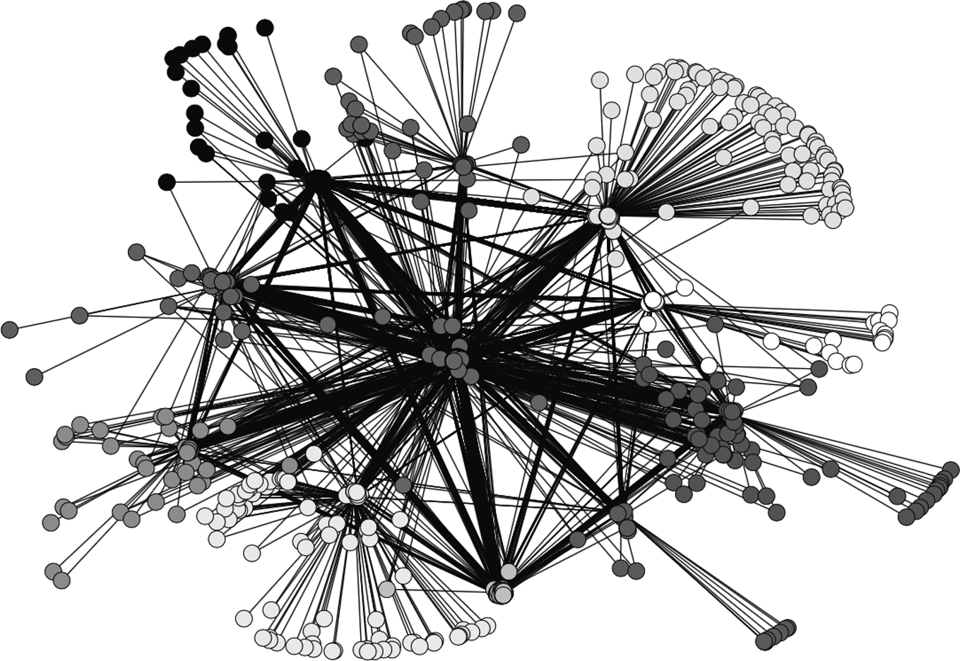
The mapping of interbank networks has been done for several countries, notably by Sheldon and Maurer (1998) for Switzerland; Inaoka et al. (2004) for Japan (BoJ-NET); Furfine (2003), Soramäki et al. (2007), and Bech and Atalay (2010) for the US Federal funds market (Fedwire); Boss et al. (2004), Elsinger et al. (2006), and Puhr et al. (2012) for Austria; Degryse and Nguyen (2007) for Belgium; van Lelyveld and Liedorp (2006) and Propper et al. (2013) for the Netherlands; Upper and Worms (2004) and Craig and von Peter (2014) for Germany; De Masi et al. (2006), Iori et al. (2008), and Finger et al. (2013) for the Italian based e-MID; Cont and Wagalath (2013), Tabak et al. (2010a) for Brazil; Wells (2004) and Langfield et al. (2014) for the United Kingdom; Martinez-Jaramillo et al. (2014) for Mexico; León (2015) for Colombia. In Fig. 1 we show an example of the typical shape of the interbank network. Specifically, we show the Austrian interbank market investigated in Boss et al. (2004). These studies of the interbank market have revealed a number of stylized facts and regularities. Interbank networks are sparse and display fat tailed degree distributions, with most banks attracting a few connections, and few banks concentrating most of the connections. While some papers identify a scale-free degree distribution (Boss et al., 2004; Inaoka et al., 2004; Soramäki et al., 2007; Propper et al., 2013; Bech and Atalay, 2010; Bargigli, 2014; León, 2015), others have reported heterogeneity but observe a departure from a strict power-law distribution of links (Martinez-Jaramillo et al., 2014; Craig and von Peter, 2014; Fricke and Lux, 2014; in't Veld and van Lelyveld, 2014) and propose to model the interbank market in terms of a core periphery network.

It might be worth noting that the fact that it is difficult to discriminate between a power-law scale free distribution and a core periphery network is not an accident of the empirical investigations performed in the interbank market. There are two important reasons explaining why it might be so difficult to discriminate between the two different models in empirical data. The first reason is that in empirical data a finite cut-off of a scale free distribution is unavoidable in finite systems and therefore empirically detected scale free distribution are typically observed only for a limited number of decades of the degree. The second reason is a theoretical reason that it is related to a mathematical property associated with a scale free system. In fact it has been proved by Chung and Lu (2002) that power-law random graphs with degree distribution proportional to k−β$k^{-\beta }$$k^{-\beta }$ with exponent β in the interval $[2,3]$ (including therefore scale free networks) almost surely contain a dense subgraph (i.e. a core) that has short distance to almost all other nodes. Therefore, also random scale free networks are almost surely characterized by the presence of a core in it. This fact makes the empirical discrimination between a scale free and a core periphery model difficult to asses because, due to the presence of a “core” also in the scale free network, core periphery or scale free can be quantified closely by a fitness indicator (see, for example, the comparison provided in Craig and von Peter, 2014 by using data of the German interbank market and simulations).

Interbank networks show disassortative mixing with respect to the bank size, so small banks tend to trade with large banks and vice versa; clustering coefficients are usually small and interbank networks satisfy the small-world property.³ Tabak et al. (2010a), Craig and von Peter (2014), Fricke and Lux (2014), and in't Veld and van Lelyveld (2014) point to a correlation between the size of financial institutions and their position in the interbank funds hierarchy in the respective Brazilian, German, Italian, and Dutch interbank markets. In these markets large banks tend to be in the core, whereas small banks are found in the periphery. The cores of the networks, composed of the most connected banks, processed a very high proportion of the total value of credit.

The dynamical evolution of interbank networks, as the subprime crisis unfolded, has been closely monitored in an attempt to identify early-warning signals of the building up of systemic risk. Fricke and Lux (2015) and Squartini et al. (2013) have analyzed respectively the e-MID market and the Dutch market. In both markets the networks only display an abrupt topological change in 2008, providing a clear, but unpredictable, signature of the crisis. Nonetheless, when controlling for banks' degree heterogeneity, Squartini et al. (2013) show that higher-order network properties, such as dyadic and triadic motifs, revealed a gradual transition into the crisis, starting already in 2005. Although these results provide some evidence of early warning precursors based on network properties, at least for the Dutch interbank market, a clear economic interpretation for the observed patterns is missing.

3.3 Multilayer Networks

When institutions are interconnected trough different types of financial contracts, such as loans of different maturities, derivatives, foreign exchange and other securities, it is critical to go beyond single-layer networks to properly address systemic risk. Multilayer networks explicitly incorporate multiple channels of connectivity and constitute the natural environment to describe systems interconnected through different types of exposures.

Taking into account the multilayer nature of networks can modify the conclusions on stability reached by considering individual network layers (see Boccaletti et al., 2014 and Kivela et al., 2014 for recent reviews). Contrary to what one would expect, the literature shows that the coupling of scale free networks may yield a less robust network (Buldyrev et al., 2010). In the case of single-layer networks, scale free networks are known to be much more robust to random failures than networks with a finite second moment e.g. of Poisson networks. Indeed, scale free networks continue to have a giant component even if most of the nodes are initially damaged. A finite percolation threshold in these networks is a finite size effect, i.e. the percolation threshold disappears in the limit when the network size becomes large. The robustness of multilayer networks can be evaluated by calculating the size of their mutually connected giant component (MCGC). The MCGC of a multilayer network is the largest component that remains after the random damage propagates back and forth thought the different layers. The percolation threshold for the mutually connected component is finite also for multiplex networks formed by layers of SF networks as in the case of a multiplex in which the layers are formed by Poisson networks. Exceptions to this finding would occur when the number of links (i.e. the degree) of interdependent participants coincides across the layers. That is, scale free networks robustness is likely to be preserved if positively correlated layers exist, such that a high-degree vertex in one layer likely is high-degree in the other layers as well (Kenett et al., 2014).

A number of financial markets have been characterized as multilayer networks. Montagna and Kok (2016) model interbank contagion in the Eurozone with a triple-layer multiplex network consisting of long-term direct bilateral exposures, short-term bilateral exposures, and common exposures to financial assets. Bargigli et al. (2015) examine a unique database of supervisory reports of Italian banks to the Banca d'Italia that includes all interbank bilateral exposures broken down by maturity and by the secured and unsecured nature of the contract. The authors found that layers have different topological properties and persistence over time.

Cont et al. (2013) use a set of different kinds of interbank exposures (i.e. fixed-income instruments, derivatives, borrowing, and lending) and study the potential contagion in the Brazilian market. Poledna et al. (2015) identify four layers of exposure among Mexican banks (unsecured interbank credit, securities, foreign exchange and derivative markets). Aldasoro and Alves (2015) analyze the multiplex networks of exposure among 53 large European banks. Langfield et al. (2014) analyze of different layers of the UK interbank system.

León (2015) studies the interactions of financial institutions on different financial markets in Colombia (sovereign securities market, foreign exchange market, equity, derivative, interbank funds). The approximate scale free connective structure of the Colombia interbank market is preserved across the layers in the multilayer mapping with financial institutions that are “too connected to fail” that are present across many of the network layers. This positive correlated multiplexity, coupled with the ultra-small world nature of the networks analyzed, suggest that the role of too connected financial institutions is critical for the stability of the market, not only at the single layer level, but for the market overall.

While a multilayer representation provides a more accurate characterizing the financial system, studies so far have mostly performed a comparison between the different layers. Future steps would require investigating the interconnections and interdependencies between these different layers and the implications of these interdependencies for financial stability.

3.4 Financial Regulations and Network Control

Of critical importance in macro-prudential policy is the identification of key players in the financial network. In September 2009, the G20 leaders requested the Financial Stability Board (FSB)⁴ to designate “Global Systemically Important Financial Institutions” (G-SIFIs). As a result, the FSB, IMF, and BIS cooperatively adopted the three valuation points – size, interconnectedness, and substitutability – as the evaluation criterion for G-SIFIs (IMF-BIS-FSB, 2009).

As we have discussed, financial networks are often characterized by skewed degree distributions, with most financial firms displaying few connections, and few financial firms concentrating many connections. In these networks the failure of a participant will have significantly different outcomes depending on which participant is selected. Those participants who are “close” (according to some measure of distance) to all other participants in the network can potentially generate widespread cascading failures if they default. A rising amount of financial literature has encouraged the usage of network metrics of centrality for identifying the institutions that are systemically important (Haldane and May, 2011; León and Murcia, 2013; Markose et al., 2012). In a broad sense, centrality refers to the importance of a node in the network. The centrality indicators typically used are constructed from measures of distance of a bank from the other banks in the network, where distance is expressed in terms of: (1) paths of length one, i.e. the number of incoming or outgoing links, for degree centrality; (2) geodesics (shortest) paths (no vertex is visited more than once), for betweenness; (3) walks (vertices and edges can be visited/traversed multiple times) for eigenvector centrality, Pagerank, Sinkrank, and Katz (see Appendix A for the mathematical definition of commonly used centrality measures). Another popular iterative centrality measure is hub and authority centrality. Acemoglu et al. (2015) introduced the notion of harmonic distance over the financial network to captures the propensity of a bank to be in distress when another bank is in distress. Markose et al. (2012) proposes a measure adapted from epidemiological studies (defined as the maximum eigenvalue for the network of liabilities expressed as a ratio of Tier 1 capital) to identify the most systemic financial institutions and determine the stability of the global OTC derivatives markets. Drehmann and Tarashev (2013) explore two different approaches to measuring systemic importance: one related to banks' participation in systemic events (PA) and another related to their contribution to systemic risk (GCA). The contribution approach is rooted in the Shapley value methodology, first proposed by Shapley (1953) for the allocation of the value created in cooperative games across individual players. Shapley values are portions of system-wide risk that are attributed to individual institutions. Because Shapley values are additive, the sum of these portions across the banks in the system equals exactly the level of system-wide risk. PA assigns a higher (lower) degree of systemic importance to an interbank lender (borrower) than GCA. The reason for this is that PA attributes the risk associated with an interbank transaction entirely to the lending counterparty, i.e. the counterparty that bears this risk and can eventually transfer it onto its creditors in a systemic event. By contrast, GCA splits this risk equally between the two counterparties. GCA is computed by focusing on each subsystem or subgroup of banks that belong to the entire system, and calculating the difference between the risk of this subsystem with and without a particular bank. Averaging such marginal risk contributions across all possible subsystems delivers the systemic importance of the bank.

A novel measure of systemic importance, based on the concept of feedback centrality, is the DebtRank (DR), introduced by Battiston et al. (2012) which measures the fraction of the total economic value that is potentially lost in the case of the distress (and not necessarily default) of a particular node. This method complements traditional approaches by providing a measure of the systemic importance of a bank even when default cascades models predict no impact at all. Applications of DR based stress test analysis (see Thiago et al., 2016 for the Brazilian interbank market, and Battiston et al., 2015 for the Italian interbank market) show that systemically important FIs do not need to be large and that traditional indicators of systemic risk underestimate contagion risk.

The identification of SIFIs is crucial to direct regulatory efforts and, for example, to assess the opportunity to limit institutions' exposures, set up some form of regulatory fees or capital surcharges, or to introduce an insurance fund financed through institution-specific insurance premia (Chan-Lau, 2010). Such an approach has recently also been taken in the IMF's Interim Report for the G20 (IMF, 2010), which outlines that an ideal levy on financial institutions should be based on a network model that would take into account all possible channels of contagion. The new Basel III rules (Basel Committee on Banking Supervision, 2013) in addition to higher capital requirements with a countercyclical component, and a framework for liquidity regulation, include limiting contagion risk as a new objective, in particular for SIFIs.

Several proposals have emerged with the purpose of creating the right incentives for institutions to control the risk they pose to the financial system. In the existing literature on prudential capital controls (Korinek, 2011), optimal policy measures are derived as tax wedges that could be implemented in a variety of equivalent ways. The opportunity cost of not receiving interest can be viewed as a Pigouvian tax. Along these lines, proposals have emerged to base capital requirements not on the risk of banks assets, but on banks' systemic importance, reflecting the impact their failure would have on the wider banking system and the likelihood of contagious losses occurring. Tarashev et al. (2010) set up a constrained optimization problem in which a policymaker equalizes banks' Shapley values subject to achieving a target level for the expected shortfall of assets to liabilities at the level of the system. Similarly Webber and Willison (2011) solve the constrained optimization problem for a policymaker who seeks to minimize the total level of capital in the UK banking system, subject to meeting its chosen systemic risk target. They show that optimal systemic capital requirements are increasing in balance sheet size (relative to other banks in the system), interconnectedness, and contagious bankruptcy costs. The paper illustrates, however, that risk-based systemic capital requirements derived in this way are procyclical and point to the need of approaches that would be explicitly countercyclical.

Gauthier et al. (2012) use different holdings-based systemic risk measures (e.g., marginal expected shortfall, ΔCoVaR, Shapley value) to reallocate capital in the banking system and to determine macroprudential capital requirements in the Canadian market using credit register data for a system of six banks. Alter et al. (2015) perform a similar exercise and compare the benchmark case, in which capital is allocated based on the risks in individual banks portfolios, and a system-based case, where capital is allocated based on some interbank network centrality metrics. Using the detailed German credit register for estimation, they find that capital rules based on eigenvectors dominate any other centrality measure, saving about 15 percent in expected bankruptcy costs.

Taxes imposed on banks in the form of contributions to a rescue fund have also been suggested. Markose et al. (2012) advocate a stabilization super-spreader fund, derived from her eigen-pair centrality measure. Like a ‘bail in’ escrow fund, the funds are deployed at the time of potential failure of a financial institution to mitigate tax payer bailouts of the failing bank. Similarly Zlatić et al. (2015) apply DebtRank to model cascade risk in the e-Mid market and determine a Pigouvian taxation to finance a rescue fund, which is used in the case of default of single financial players.

Poledna and Thurner (2016) and Leduc and Thurner (2017) have proposed to use a transaction-specific tax that discriminates among the possible transactions between different lending and borrowing banks. A regulator can use the systemic risk tax (SRT) to select an optimal equilibrium set of transactions that effectively ‘rewire’ the interbank network so as to make it more resilient to insolvency cascades. The SRT was introduced and its effect simulated using an agent-based model in Poledna and Thurner (2016), while Leduc and Thurner (2017) prove analytically that an SRT can be applied without reducing the total credit volume and thus without making the system less efficient. Using an equilibrium concept inspired by the matching markets literature the paper shows that the SRT induces a unique equilibrium matching of lenders and borrowers that is systemic-risk efficient, while without this SRT multiple equilibrium matchings exist, which are generally inefficient.

3.5 Stress-Test Scenario Analysis

A number of papers have used counterfactual simulations to test the stability of financial systems and assess the danger of contagion due to credit exposures in national interbank markets. The approach consists in simulating the breakdown of a single, or possibly more, banks and subsequently assess the scope of contagion. The baseline stress-test model runs as follows: a first bank defaults due to an exogenous shock; the credit event causes losses to other banks via direct exposures in the interbank market and one or more additional banks may default as a result; if this happens, a new round of losses is triggered. The simulation ends when no further bank defaults. Simulations are then repeated by assuming the unanticipated failure of a different bank, possibly spanning across the all system or focusing on the most important institutions.

Overall, the evidence of systemic risk from these tests is mixed. Risk of contagion has been reported, as a percentage of banking system's total assets lost, by Degryse and Nguyen (2007) for Belgium (20%), Mistrulli (2011) for Italy (16%), Upper and Worms (2004) for Germany (15%), and Wells (2004) for the UK (15%). By contrast, little possibility for contagion was found by Blavarg and Nimander (2002) for Sweden, Lubloy (2005) for Hungary, and Sheldon and Maurer (1998) for Switzerland. Furfine (2003) and Amundsen and Arnt (2005) also report only a limited possibility for contagion. Cont et al. (2013) show that in the Brazilian banking system the probability of contagion is small, however the loss resulting from contagion can be very large in some cases.

Recent studies have shown that not taking into account possible loss amplification due to indirect contagion associated with fire sales and bank exposures to the real sector can significantly underestimate the degree of fragility of financial system. We will discuss these effects in Sections 4.1 and 4.2.

3.6 Network Reconstruction

A major limitation of the stress-test analysis is that often the full network of interbank liabilities is not available to regulators. For most countries bilateral linkages are unobserved and aggregate balance sheet information are used for estimating counterparty exposures. Formally the problem is that the row and column sums of a matrix describing a financial network are known but the matrix itself is not known. To estimate bank-to-bank exposures, different network reconstruction methods have been proposed. The most popular approach for deriving individual interbank liabilities from aggregates has been to minimize the Kullback–Leibler divergence between the liabilities matrix and a previously specified input matrix (see Upper, 2011 for a review). This network reconstruction approach is essentially a constrained entropy maximization problem, where the constraints represent the available information and the maximization of the entropy ensures that the reconstructed network is maximally random, given the enforced constraints.

One drawback of the Maximum Entropy (ME) method is that the resulting interbank liabilities usually form a complete network. However, as we have seen, empirical research shows that interbank networks are sparse. The maximum entropy method might thus bias the results, in the light of the theoretical findings that better connected networks may be more resilient to the propagation of shocks. This is confirmed by Mistrulli (2011), who analyzes how contagion propagates within the Italian interbank market using actual bilateral exposures and reconstructed ME exposures. ME is found to generally underestimate the extent of contagion. Similarly Solórzano-Margain et al. (2013) showed that financial contagion arising from the failure of a financial institution in the Mexican financial system would be more widespread than from simulations based on reconstructed network based on ME algorithm.

Mastromatteo et al. (2012) have proposed an extension to the ME approach using a message-passing algorithm for estimating interbank exposures. Their aim is to fix a global level of sparsity for the network and, once this is given, allow the weights on the existing links to be distributed similarly to the ME method. Anand et al. (2014) have proposed the minimum density (MD) method which consists in minimizing the total number of edges that is consistent with the aggregated interbank assets and liabilities. They argue that the MD method tends to overestimate contagion, because minimize the number of links, and therefore can together with the ME method be used to provide upper and lower bounds for stress test results. However, increasing the number of links has a non-monotonous effect on the stability of a network, thus attempts to derive bounds on systemic risk by optimizing over the degree of completeness are unlikely to be successful. Montagna and Lux (2013) construct a Monte Carlo framework for an interbank market characterized by a power law degree distribution and disassortative link formation features via a fitness algorithm (De Masi et al., 2006).

The ME approach is deterministic in the sense that the method produces a point estimate for the financial network that is treated as the true network when performing stress tests. Probabilistic approaches to stress-testing have been attempted by Lu and Zhoua (2011), Halaj and Kok (2013), Squartini et al. (2017), Bargigli (2014), Montagna and Lux (2013), and Gandy and Veraart (2017). Such approaches consist in building an ensemble of random networks, of which the empirical network can be considered a typical sample. This allows to analyze not only the vulnerability of one particular network realization retrieved from the real data, but of many plausible alternative realizations, compatible with a set of constrains. However, to generate a realistic random sample it is crucial to impose the relevant constrains on the simulated networks, reproducing not just the observed exposures but also basic network properties. Cimini et al. (2015) introduce an analytical maximum-entropy technique to reconstruct unbiased ensembles of weighted networks from the knowledge of empirical node strengths and link density. The method directly provides the expected value of the desired reconstructed properties, in such a way that no explicit sampling of reconstructed graphs is required. Gandy and Veraart (2017) have proposed a reconstruction model, which, following a Bayesian approach, allows to condition on the observed total liabilities and assets and, if available, on observed individual liabilities. Their approach allow to construct a Gibbs sampler to generate samples from this conditional distribution that can be used in stress testing, giving probabilities for the outcomes of interest. De Masi et al. (2006) propose a fitness model, where the fitness of each bank is given by their daily trading volume. Fixing the level of heterogeneity the model reproduces remarkably well topological properties of the e-Mid interbank market such as degree distribution, clustering, and assortativity. Finally Iori et al. (2015) introduce a simple model of trading with memory that correctly reproduces features of preferential trading patterns observed in the e-Mid market.

An international study lead by several central banks has been conducted to test the goodness of network reconstruction algorithms (Anand et al., 2017). Initial results suggest that the performance of the tested methods depends strongly on the similarity measure used and the sparsity of the underlying network. This highlights that in order to avoid model risk arising from calibration algorithms, structural bilateral balance sheet, and off balance sheet, data are crucial to study systemic risk from financial interconnections.

Another common critique to stress test studies of contagion is the lack of dynamics in terms of banks' behavioral adjustments. Critics stress the importance to include indirect financial linkages, in terms of common exposures and business models, as well as fire sales or liquidity hoarding contagion driven by fear and uncertainty. To address these concerns, a few papers have explored the role of funding and liquidity risk via simulation experiments. The idea of liquidity risk as banks start fire-selling their assets, depressing overall prices in the market, was initially explored by Cifuentes et al. (2005) and has been further investigated in a simulation framework by Nier et al. (2007), Gai and Kapadia (2010), Haldane and May (2011), Tasca and Battiston (2016), Corsi et al. (2016), Cont and Wagalath (2013), Caccioli et al. (2014), and Poledna et al. (2014). The role of funding risk induced by liquidity hoarding is explored in Haldane and May (2011), Chan-Lau (2010), Espinosa-Vega and Solé (2011), Fourel et al. (2013), Roukny et al. (2013), and Gabrieli et al. (2014). Finally, simultaneous impact of market and funding liquidity risk is explored by Aikman et al. (2010) and Manna and Schiavone (2012).

While this body of work has considerably improved our understanding of the effects of the networks structure on the spreading of systemic risk unfortunately data on a range of relevant activities (securities lending, bilateral repos, and derivatives trading) remain inadequate. Moreover, the activities of non-bank market participants, such as asset managers, insurance and shadow banks, and their interconnections remain opaque. A proper assessment of systemic risk relies on a better understanding of the business models of these players and their interactions and on enhanced availability of individual transactions data.

3.7 Econometrics Systemic Risk Measures

Due to limited availability of supervisory data to capture systemic risk stemming from contagion via bilateral exposures, approaches have been suggested to derive systemic risk from available market data. A number of econometric measures, beyond Pearson correlation, have been proposed to measure the degree of correlation and concentration of risks among financial institutions, and their sensitivity to changes in market prices and economic conditions. Popular ones include Value-at-Risk (CoVaR) by Adrian and Brunnermeier (2016), CoRisk by Chan-Lau (2010), marginal and systemic expected shortfall by Acharya et al. (2012), distressed insurance premium by Huang et al. (2012), SRISK by Brownlees and Engle (2016), distance to distress by Castren and Kavonius (2009), and POD (probability that at least one bank becomes distressed) by Goodhart and Segoviano Basurto (2009). While these approaches are not network based, they are briefly mentioned here (see Appendix B for technical definitions) for completeness as they provide complementary methodologies to assess systemic risk and financial fragility. The underlying assumption behind these “market based” systemic risk measures is that the strength of relationships between different financial institutions, based on correlations between their asset values, is related to the materialization of systemic risk. The rationale is that common movements in underlying firms' asset values are typically driven by the business cycle, interbank linkages or shift in market sentiment that affects the valuation of bank assets simultaneously. By assuming that these are likely causes of contagion and common defaults, systemic risk should be captured by the correlations of observable equity returns.⁵ However the importance of short-term changes to market data might be overestimated, and the mechanisms that lead to the realization of systemic defaults are not well understood. In particular, when markets function poorly, market data are a poor indicator of financial environments. Correlations between distinct sectors of the financial system became higher during and after the crisis, not before, thus during non-crisis periods, correlation play little role in indicating a build-up of systemic risk using such measures. Moreover, measures based on probabilities invariably depend on market volatility, and during periods of prosperity and growth, volatility is typically lower than in periods of distress. This implies lower estimates of systemic risk until after a volatility spike occurs, which reduces the usefulness of such a measure as an early warning indicator. Overall these measures may be misleading in the build up to a crisis as they underprice risk during market booms.

3.8 Location Advantages in Interbank Networks

In addition to having implications for financial stability, holding a central position in the interbank networks, or establishing preferential relationships, may lead to funding benefit. The exploration of potential location advantages has been the focus of recent papers. Bech and Atalay (2010) analyze the topology of the Federal Funds market by looking at O/N transactions from 1997 to 2006. They show that reciprocity and centrality measures are useful predictors of interest rates, with banks gaining from their centrality. Akram and Christophersen (2013) study the Norwegian interbank market over the period 2006–2009. They observe large variations in interest rates across banks, with systemically more important banks, in terms of size and connectedness, receiving more favorable terms. Temizsoy et al. (2017) show that network measures are significant determinants of funding rates in the e-MID O/N market. Higher local measures of centrality are associated with increasing borrowing costs for borrowers and decreasing premia for lenders. However, global measures of network centrality (betweenness, Katz, PageRank, and SinkRank) benefit borrowers who receive a significant discount if they increase their intermediation activity, while lenders pay in general a premium (i.e. receive lower rates) for centrality. This effect is interpreted by the authors, as driven by the market perception that more central banks will be bailed out if in distress, because “too connected to fail”. The expectation of implicit subsidies could create moral hazard and provide incentives for banks to become systemically important, exacerbating system fragility. Thus Temizsoy et al. (2017) suggest that monitoring how funding cost advantages evolve over time can act as an effective early warning indicator of systemic risk and provide a way to measure the effectiveness of regulatory policy to reduce the market perception that systemically important institutions will not be allowed to default.

During the crisis, increased uncertainty about counterpart credit risk led banks to hoard liquidity rather than making it available in the interbank market. Money markets in most developed countries almost came to a freeze and banks were forced to borrow from Central Banks. Nonetheless there is growing empirical evidence that banks that had established long term interbank relationships had better access to liquidity both before and during the crisis (Furfine, 2001; Cocco et al., 2009; Liedorp et al., 2010; Affinito, 2012; Brauning and Fecht, 2012; Temizsoy et al., 2015).

Early papers on interbank markets focus on the existence of lending relationships in the US Federal Funds markets (Furfine, 1999, 2001). Furfine (1999) shows that larger institutions tend to have a high number of counterparties while Furfine (2001) finds that banking relationships have important effects on borrowing costs and longer relationship decreases the interest rate in the funds market. Affinito (2012) uses data from Italy to analyze interbank customer relationships. His findings are that stable relationships exist and remain strong during the financial crisis. Liedorp et al. (2010) examine bank to bank relationships in the Dutch interbank market to test whether market participants affect each other riskiness through such connections. They show that larger dependence on interbank market increases risk, but banks can reduce their risk by borrowing from stable neighbors. Brauning and Fecht (2012) show that German lenders anticipated the financial crisis by charging higher interest rates in the run-up to the crisis. By contrast, when the sub-prime crisis kicked in, lenders gave a discount to their close borrowers, thus pointing to a peer monitoring role of relationship lending. Temizsoy et al. (2015) analyze the structure of the links between financial institutions participating in the e-MID interbank market. They show that, particularly after the Lehman's collapse, when liquidity became scarce, established relationships with the same bank became an important determinant of interbank spreads. Both borrowers and lenders benefited from establishing relationship throughout the crisis by receiving better rates from and trading larger volume with their preferred counterparties.

Cocco et al. (2009) suggest that size may be the main factor behind the Portuguese interbank funds connective and hierarchical architecture. Small banks acting as borrowers are more likely to rely on lending relationship than larger banks. Thus they suggest that financial institutions do not connect to each other randomly, but rather interact based on a size-related preferential attachment process, possibly driven by too-big-to-fail implicit subsidies or market power.

Hatzopoulos et al. (2015) have investigated the matching mechanism between lenders and borrowers in the e-MID market and its evolution over time. They show that, when controlling for bank heterogeneity, the matching mechanism is fairly random. Specifically, when taking a lender who makes l transactions over a given period of time and a borrower who makes b transaction over the same period, and such that they have m trades in common over that period, Hatzopoulos et al. (2015) show that m is consistent with a random matching hypothesis for more than 90% of all lender/borrower pairs. Even though matches that occur more often than those consistent with a random null model (which they call over expressed links) exist and increase in number during the crisis, neither lenders nor borrowers systematically present several over expressed links at the same time. The picture that emerges from their study is that banks are more likely to be chosen as trading partners because they are larger and trade more often and not because they are more attractive in some dimension (such as their financial healthiness).

Overall the empirical evidence suggests that, particularly at a time of deteriorating trust towards credit rating agencies, private information acquired through repeated transactions plays an important role in mitigating asymmetric information about a borrower's creditworthiness and can ease liquidity redistribution among banks. These results show that interbank exposures are used as a peer-monitoring device. Private information acquired through frequent transactions, supported liquidity reallocation in the e-MID market during the crisis by improving the ability of banks to assess the creditworthiness of their counterparties. Relationship lending thus play a positive role for financial stability and can help policymakers to assess market discipline. Furthermore, the analysis of patterns of preferential relationships may help identifying systemically important financial institutions. If a bank, who is the preferential lender to several borrowers defaults, or stop lending, this may pose a serious funding risk for its borrowers who may find it difficult to satisfy their liquidity needs from other lenders and may be forced to accept deals at higher rates. This may eventually put them under distress and increase systemic risk in the system. Similarly if preferential borrowers exit the interbank market, such lenders may find it difficult to reallocate their liquidity surplus if they fail to find trusted counterparties. The resulting inefficient reallocation of liquidity, may in turn increase funding costs of other borrowers and again contribute to the spread of systemic risk. In this sense relationship lending provides a measure of the financial substitutability of a bank in the interbank market. Thus when establishing if a bank is too connected to fail, regulators should not only look at how connected a bank is, but also at how preferentially connected it is to other players. Finally, reliance on relationship lending is an indicator of trust evaporation in the banking system and monitoring the effect of stable relations on spreads and traded volume may help regulators to identify early warning indicator of a financial turmoil.

4.1 Proximity Based Networks

In proximity based networks a similarity or a dissimilarity measure (i.e. technically speaking a proximity measure, see a reference text of Data Mining for a formal definition as, for example, Han et al., 2011) computed between all pairs of elements of a system is used to determine a network. The network obtained highlights the most relevant proximities observed in the system. Let us make an example to clarify the concept. Let us consider two banks having no credit relationship in the interbank market connecting them in a given time period. Is this meaning that the two banks are isolated the one to the other unless a chain of bankruptcy of banks occurs? The general answer is no. We can see this by considering the fact that the two banks have both a portfolio of assets and that the two portfolios can present a given degree of similarity. Two banks characterized by a high degree of similarity of their portfolios will be impacted by market dynamics and by exogenous news in a similar way in spite of the fact that they do not present direct credit relationship. For example, the fire sale of a distressed bank of a given asset will impact all those banks having large weights of that asset in their portfolios. The interlinkages associated with different degree of similarity of the set of elements of a given system can therefore be summarized and visualized in a network. In the literature these networks are sometime called with different names. For example, in neuroscience they are called functional networks because they are obtained starting from the functional activity detected by functional magnetic resonance signals detected in different regions of the brain. The proximity can be estimated by considering features of the considered elements that can be numeric, binary or even categorical.

4.1.1 The Minimum Spanning Tree

The first example of proximity based network was introduced in Mantegna (1999). This study proposed to obtain a network starting from a dissimilarity measure estimated between pairs of stocks traded in a financial market. A dissimilarity measure between two financial stocks can be obtained by first estimating the Pearson correlation coefficient ρ between the two time series of return of stocks and then obtaining a dissimilarity d (more precisely a distance) through the relation $d=\sqrt{2(1-\rho )}$. By following this approach, one can always associate a similarity or dissimilarity matrix to any multivariate time series and use this matrix to define a weighted complete network. The weight of each link being the value of the proximity measure.

For this type of weighted complete networks all information which is present in the proximity matrix is retained and it has associated the same degree of statistical reliability. However, in real cases this ideal condition is hardly verified. In fact, not all the information present in a proximity matrix has the same statistical reliability. The specific level of reliability depends on the way the proximity measure is obtained and limitations are always present when the estimation of the proximity measure is done with a finite number of experimental records or features. The unavoidable presence of this type of limitation is quantified by random matrix theory (Metha, 1991) in a very elegant way. For example, the eigenvalue spectrum of the correlation matrix for a random Gaussian multivariate set is given by the Marčenko–Pastur distribution (Marčenko and Pastur, 1967). Several studies have shown that the Marčenko–Pastur distribution computed for a correlation matrix of n stocks with a finite number of records widely overlaps with the ones empirically observed in financial markets although also clear deviations from this null hypothesis are observed (Laloux et al., 1999; Plerou et al., 1999).

In empirical analyses, it is therefore important and informative to perform a meaningful filtering of any proximity matrix obtained from a multivariate system described by a finite number of records or features. One of the most effective filtering procedures of a proximity matrix is the extraction from it of its minimum (for dissimilarity) or maximum (for similarity) spanning tree (Mantegna, 1999). The minimum spanning tree is a concept of graph theory and it is the minimum (or maximum) tree connecting all the nodes of a system through a path of minimal (maximal) length. The minimum spanning tree can be determined by using Prim's or Kruskal's algorithms. The information it selects from the original proximity measure is related to the hierarchical tree that can be obtained from the same proximity matrix by using the hierarchical clustering procedures known as single linkage. For more details about the extraction of minimum spanning trees from a proximity matrix one can consult (Tumminello et al., 2010).

In Fig. 2 we show an example of minimum spanning tree obtained for a set of 100 highly capitalized stocks traded in the US equity markets during the time period January 1995–December 1998. In the MST several stocks, such as, for example, BAC (Bank of America Corp.), INTC (Intel Corp.), or AEP (America Express), are linked with several stocks belonging to the same economic sector (financial, technology, and utility sector respectively) whereas others (the most notable case is General Electric Company (GE)) are linked to stocks of different sectors. In general the clustering in terms of economic sectors of the considered companies is rather evident. Since the original proposal of Mantegna (1999), minimum spanning trees have been investigated in a large number of empirical studies involving different financial markets operating worldwide or in diverse geographical areas. The classes of assets and geographically located markets investigated through the proximity based network methodology comprises⁶: stocks traded in equity markets geographically located in US (Mantegna, 1999; Bonanno et al., 2001; Onnela et al., 2002; Miccichè et al., 2003; Bonanno et al., 2003; Onnela et al., 2003; Precup and Iori, 2007; Eom et al., 2007; Tumminello et al., 2007; Brida and Risso, 2008; Zhang et al., 2011), in Europe (Coronnello et al., 2005), in Asia (Jung et al., 2006; Eom et al., 2007; Zhuang et al., 2008), market indices of major stock exchanges (Bonanno et al., 2000; Coelho et al., 2007; Gilmore et al., 2008; Song et al., 2011), bonds and interest rates (Di Matteo and Aste, 2002; Dias, 2012, 2013), currencies (McDonald et al., 2005; Mizuno et al., 2006; Górski et al., 2008; Jang et al., 2011; Wang et al., 2012, 2013), commodities (Sieczka and Holyst, 2009; Barigozzi et al., 2010; Tabak et al., 2010b; Kristoufek et al., 2012; Zheng et al., 2013; Kazemilari et al., 2017), interbank market (Iori et al., 2008), housing market (Wang and Xie, 2015), credit default swaps market (León et al., 2014).

As for other data mining approaches, there are multiple approaches to perform information filtering. The choice of specific approach depends on the posed scientific question and on the ability of the filtering process to highlight the information of interest. This is similar to the case of hierarchical clustering where there is no a priori recipe to select the most appropriate algorithm performing the clustering. In addition to the approach of the minimum spanning tree several other approaches have been proposed in the literature to perform information filtering on networks. We will discuss some examples in the following subsection.

4.2 Association Networks

Another class of networks is the class we name association networks. In this type of networks two nodes of a complex system are connected in a network by computing a quantity that is putting in relation node i with node j of a given system. The quantity computed can be a complex indicator as, for example, the partial correlation between the time evolution of node i with node j or an indicator of the rejection of a statistical test against a given null hypothesis.

A prominent example of association network is the partial correlation network investigated in Kenett et al. (2010). Partial correlation is a measure of how the correlation between two variables, e.g., stock returns, is affected by a third variable. Kenett et al. (2010) define a proxy of stock influence, which is then used to construct a partial correlation network. The empirical study performed on stocks traded at the US equity markets concluded that stocks of the financial sector and, specifically, of investment services sub-sector, are taking a special position in the association network based on partial correlation. Partial correlation networks have also been investigated by Anufriev and Panchenko (2015) for publicly traded Australian banks and for their connections to domestic economic sectors and international markets.

In their paper, Billio et al. (2012) propose a method to construct a directed network starting from a statistical test performed between each pair of time series of a multivariate system. Specifically they investigate Granger-causality between monthly return time series, and starting from the time series they infer a network of dependencies of hedge funds, publicly traded banks, broker/dealers, and insurance companies. In other words an association network of Granger-causal relations among these institutions is identified via the pairwise Granger-causality test. Granger causality is a statistical notion of causality based on the forecast power of two time series. Time series j is said to “Granger-cause” time series i if past values of j contain information that helps predict i above and beyond the information contained in past values of i alone. In their investigation authors conclude that their results show a pronounced asymmetry in the degree of connectedness among hedge funds, publicly traded banks, broker/dealers, and insurance companies sectors, with banks playing a much more important role in transmitting shocks than other financial institutions.

Another example of association networks concerns the networks obtained when performing pairwise co-integration tests. First attempts to produce association networks based on pairwise co-integration test are reported in Yang et al. (2014) and Tu (2014).

The need of many statistical tests to be used for the construction of an association network raises some problems directly originating form the pairwise nature of the performed tests. For example, in the case of Granger-causality test, as pointed out by Basu et al. (2017), direct pairwise estimation does not take into account indirect effects on the pair under consideration. For example in a system with 3 nodes and 2 “true” Granger causal dependencies: $B\to C,C\to A$, a Granger causal test would detect an additional (spurious) pairwise Granger causal effect $B\to A$, due to indirect effect through C. In fact a similar concern arises with the use of CoVaR, since these models estimate the covariance of an institution with the rest of the system without conditioning it on all other participants. Such inconsistency may impose large economic costs; for example, a number of institutions that are not highly interconnected may end up being wrongly classified as inter-connected under such approaches.

To address this problem Basu et al. (2017) develop and estimate a measure of network connectivity that explicitly recognizes the possibility of connectivity of all the firms in the network, in contrast with extant measures of systemic risk that, either explicitly or implicitly, estimate such connections using pair-wise relationships between institutions. The system-wide approach, is based on the Lasso penalized Vector Auto-Regression (LVAR) model that only focuses on estimating the strongest interconnections, while forcing weaker relationships to zero. Basu et al. (2017) also consider explicitly the problem of the control of the family-wise error rate. In fact when a large number of statistical tests are performed to obtain an association network the absence of the control of the family-wise error rate can produce a large number of false positive. This problem was first recognized in Tumminello et al. (2011) where the concept of the so-called statistically validated network was introduced (see next section). In Tumminello et al. (2011) it was shown that the so-called Bonferroni correction is highly precise but often characterized by low power and therefore associated with a relatively low accuracy. For this reason, as it is common in statistical approaches needing a control of the family-wise error rate the approach based on the control of the false discovery rate (Hochberg and Tamhane, 1987) was proposed.

A similar system-wide approach was developed in Diebold and Yimaz (2014). However the Diebold and Yimaz (2014) approach requires fitting full vector autoregressive models, simultaneously for all firms, and use variance decomposition of the forecast error of the fitted model to define the network topology and extract connectivity measures. Since the number of parameters to be estimated, even for the simplest lag-1 VAR model in this approach is quadratic in the number of institutions under consideration, the model can only be estimated for a limited number of firms (15 in Diebold and Yimaz, 2014). The advantage of the LVAR model lays on the fact that it needs significantly lower number of time points to estimate as long as the underlying network is approximately sparse, and can be applied to more realistic setting involving all important banks of the economy.

Barfuss et al. (2016) have recently introduced an information filtering methodology (LoGo) to produce parsimonious models associated with a meaningful structure of dependency between variables of interest. The strength of this methodology is that the global sparse inverse covariance matrix is produced from a simple sum of local inversions. This makes the method computationally very efficient and statistically robust. Applied to financial data the method results computationally more efficient than state-of-the-art methodologies such as Glasso producing, in a fraction of the computation time, models that can have equivalent or better performances but with a sparser inference structure.

4.3 Statistically Validated Networks

In the previous section we have seen that a statistical test is performed to asses the existence of an undirected or directed link between each pair of nodes of the system in the study of association networks. Moreover, a statistical validation procedure can also be performed in ordinary networks to detect those links that are presenting marked differences from a given null hypothesis. According to Tumminello et al. (2011), when statistical tests are performed to highlight specific links (or the absence of links) between pairs of nodes of the investigated systems, we say we are in the presence of statistically validated networks detected against a given null hypothesis. The value of this statistical approach primarily relies on the fact that most systems of interest are highly heterogeneous with respect to economic or financial actions taken in a given period of time (e.g. number of loans, number of syndicated loans, amount of loans provided to firms, etc.) and therefore detecting over-expression or under-expression of interaction with respect to a null hypothesis taking into account for the heterogeneity of the action of each node can highlight important properties of the analyzed system.

The first example of statistical validation in weighted network is the work of Serrano et al. (2009). In this paper the statistical validation is performed on the outgoing weight of each node of the network statistically compared with a null hypothesis of uniform distribution of the total node strength in the outgoing arcs. In their paper authors statistically validate each link by deciding, which of the links carry disproportionate fraction of the weights of a given node. Specifically they compare the empirical value of each link of a node with a null model that considers all links of each node as equally probable. By performing the statistical validation node-by-node they select only those links that reject the null hypothesis therefore obtaining what they call the “multiscale backbone” of the system. It is worth noting that the method is not affected by the heterogeneity of the strength of nodes allowing for a selection of nodes working at all scales of the weight of links. Their approach was then generalized to the case of non-uniform distribution of weights by Radicchi et al. (2011).

Heterogeneity is a typical fingerprint of almost all complex systems. Economic and financial systems do not deviate from this general property and in fact economics was one of the first disciplines where power law distributions were documented and modeled. Vilfredo Pareto discovered a power law distribution in the wealth distribution of individuals in many countries and historical time periods as early as in 1897 (Pareto, 1897). An indication about the essential heterogeneity of economic and financial systems can be seen in the observation that the majority of economic and financial networks are presenting a degree distribution with a pronounced level of leptokurtosis. This observation has motivated network scientists to investigate complex network by estimating the deviation observed from the basic heterogeneity observed in the system.

The first approach designed to perform statistical tests of the over-expression of a given node action (e.g. participating to a credit relationship, performing a market transaction, etc.) against a null hypothesis taking into account the heterogeneity of the nodes was first presented for undirected interaction in Tumminello et al. (2011) and then extended to directed interaction and to the investigation of under-expression of interactions in Hatzopoulos et al. (2015). The method is designed for complex systems where two sets of agents repeats an action involving two actors a number of times in a given time interval. For example the two sets of agents can be (i) calling mobile phone subscribers and (ii) receiving mobile phone subscribers. Another example is the one where the two sets of agents are (i) lending banks and (ii) borrowing banks in the interbank market. Usually these complex systems are highly heterogeneous systems and therefore detecting links that are rejecting a null hypothesis taking into account the heterogeneity of the activity of each node in a statistical test can highlight informative interlinkages of the investigated system. In Fig. 3 we show the statistically validated network of the Italian segment of the e-MID market obtained in Hatzopoulos et al. (2015) from data of the maintenance period from 10 September 2008 to 9 December 2008.

It should be noted that the methodology used to obtain a statistically validated network needs performing a large number of statistical tests, that are usually done on all links of a large network. These means that this statistical procedure needs the so-called control of family-wise error rate. Tumminello et al. (2011) were the first pointing out the need of multiple hypothesis test correction when statistical tests are used to select or construct networks. Family-wise errors arise from the fact that when a large number of statistical tests are simultaneously performed a certain number of false positive are unavoidably observed due to the parallel repetition of the statistical test many times.

There are different types of procedures to correct multiple hypothesis testing procedures to avoid the presence of false positive. The most restrictive multiple hypothesis test correction is the so-called Bonferroni correction (Hochberg and Tamhane, 1987) that is performed by setting the statistical threshold as ${\alpha }_B=\alpha /N_t=0.01/N_t$, where α is the chosen univariate statistical threshold and $N_t$ is the number of tests to be performed. The Bonferroni correction controls the number of false positive therefore ensuring a high degree of statistical precision to the multiple hypothesis test performed. Unfortunately, in some cases it does not guarantee sufficient statistical accuracy because it may provide a large number of false negative. The procedure controlling the false discovery rate introduced in Benjamini and Hochberg (1995) reduces the number of false negative by controlling the expected proportion of rejected null hypothesis without significantly expanding the number of false positive. For this reason the multiple hypothesis test correction controlling the false discovery rate is today widely used also when investigating statistically validated or association networks.

Statistically validated networks originating from bipartite networks have been investigated in a variety of systems. The methodology was first illustrated by investigating the bipartite relationship between genomes and proteins in simple organisms, the price dynamics of financial stocks described in terms of categorical variables and the Internet Movie Database (Tumminello et al., 2011). It has also been used to detect and classify investment strategies of single investors (Tumminello et al., 2012). The methodology is rather flexible and easily adapted to directional relationships such as the ones of any form of communication from a caller to a receiver, any form of loan provided from a lender to a borrower or any form of market transaction from a seller to a buyer, etc. With this generalization of the methodology statistically validated networks have been detected and analyzed in mobile phone communication networks (Li et al., 2014a, 2014b) and in the empirical investigation of the e-MID interbank market (Hatzopoulos et al., 2015).

5.1 Overlapping Portfolios and Feedback Effects

Systemic risk is the research area where the use of event or relationship networks and proximity based networks is jointly required for a realistic model of the financial system. In fact, both direct and market mediated indirect channels of contagion need to be taken into account for the estimation of systemic risk of the financial system. One indirect channel can be highlighted by estimating the amount of overlapping of portfolios of different institutions. Market impact of portfolio deleveraging in stress scenarios can in fact induces contagion paths that are indirect (Cont and Wagalath, 2013; Huang et al., 2013; Caccioli et al., 2014). The magnitude of these additional market mediated contagion paths depends on the portfolios overlap of economic actors acting in the financial system (Cifuentes et al., 2005; Braverman and Minca, 2014; Cont and Schaanning, 2017). The most prominent aspect of this approach concerns fire sales occurring during market downturns. It is documented that financial institutions in the presence of financial distress can be forced to fire sales of assets (Kyle and Xiong, 2001; Manconi et al., 2012; Cont and Wagalath, 2013). Due to market impact fire sales can generate a positive feedback loop that will increase endogenous risk (Shin, 2010) creating a channel of contagion for those financial institutions with high similarity in the holding of given assets.

Recent papers have proposed possible methods to include fire sales induced contagion channels into macro-stress tests (Duarte and Eisenbach, 2015; Greenwood et al., 2015; Cont and Schaanning, 2017). In Duarte and Eisenbach (2015) authors construct a systemic risk measure quantifying vulnerability to fire-sale spillovers using detailed regulatory balance sheet data for US commercial banks and repo market data for broker-dealers. They find that fire sale externalities can be substantial, even for moderate shocks in normal times. For example, they estimated that for commercial banks a 1 percent exogenous shock to assets in 2013 in the first quarter can produce fire sale externalities of the order of 21 percent of system capital. Greenwood et al. (2015) introduced a model where fire sales propagate shocks across bank balance sheets. Authors showed how this contagion spreads across the banking sector, and how it can be estimated empirically using balance sheet data. In particular, authors computed bank exposures to system-wide deleveraging, as well as the spillovers induced by individual banks. The study presents an application to European banks. Cont and Schaanning (2017) suggest an operational framework able to quantify the impact of deleveraging in stress scenarios when the financial institutions are subjected to portfolio constraints. The authors show that this price mediated loss contagion may be quantified through a liquidity-weighted overlaps across portfolios. The paper also performs a case study using data on European banks. By performing the case study authors show that indirect contagion effects affect the outcome of bank stress tests and lead to heterogeneous losses of banks which cannot be replicated in a stress test without deleveraging effects. The study highlights the difference between insolvency and illiquidity clarifying that the presence of different levels of illiquidity and insolvency can lead to substantially different loss estimates compared to standard models just based on leverage targeting.

Risk metrics based on the mechanism of portfolio rebalancing through fire sales require the full knowledge of the portfolio holdings of each institution in the economy. However, such detailed information may not be available, especially at frequency higher than a quarter. Di Gangi et al. (2015) propose to apply the maximum entropy approach to the inference of the network of portfolio weights in order to estimate metrics of systemic risk due to fire sales spillovers, starting form a reduced information set. The authors show that this approach, while underestimating systemic risk in interbank networks (Mistrulli, 2011), works well when applied to reconstruct the exposures of US commercial banks available via FFIEC Call Reports. Gualdi et al. (2016) propose a method to assess the statistical significance of the overlap between heterogeneously diversified portfolios, in order to investigate patterns of portfolio overlap. When applied to a historical database of SEC 13-F filings, the authors find that the proposed proxy of fire sale risk, after reaching a peak in 2008 had subsequently decreased. However fire sale risk has been increasing again from 2009 to the end 2013 and the number of securities that can be involved in a potential fire sale has been steadily growing in time, with an even stronger proliferation of contagion channels.

5.2 Financial Sector and the Real Economy

Another important channel of indirect contagion of banks due to external shocks is the indirect channel due to common exposure to firms. When a large firm get distressed it will present difficulties in paying back the loans obtained from a number of banks. In other words the links existing from the real economy to the financial sector can act as channels of contagion from a firm or a set of firms to the banking system especially in a period of economic crisis when a state of financial distress may impact simultaneously many firms or firms of an entire economic sub-sector. The impact of the bank–firm network on systemic risk and its role as channel of contagion is investigated theoretically in Lux (2016). In this study, the author proposes a stochastic model of a bipartite credit network observed between banks and the non-bank corporate sector. The model is based on stylized facts observed empirically in large data sets of bank–firm loans for some countries. The model is investigated computationally and it shows a pronounced non-linear behavior under shocks. In fact, the default of a single unit will typically have no immediate avalanche effect, but might lead to a wide collapse of the entire system in a certain number of cases. The model and its numerical investigations suggest that when one distinguishes between contagion due to interbank credit and due to joint exposures to counterparty risk via loans to firms, the later channel appears more important for contagious spread of defaults. Other recent papers that assess how the interbank network structure affects lending to the wider economy via macro-finance ABM simulations are Gabbi et al. (2015) and Gurgone et al. (2017). In the first paper, firms behavior is exogenous and stochastic, and lending to firms short term. In the second firm dynamics are endogenized, lending to firms is long term, and banks implement precautionary liquidity hoarding strategies. Both papers show that constrains to interbank lending affect rates and volumes on the bank–firm credit markets. Instability arising from this channel dominates direct knock-on effects. However, the connectivity of the interbank market has a non-monotonous effect on macro-financial stability.

Starting from 2010 a series of empirical studies have considered the structure of the bank–firm network observed by considering the credit network provided by the banking system of to the firms operating in a given country. The first studies were conducted by analyzing the credit relations of Japanese banks with large Japanese firms (De Masi et al., 2011), and a subset of the Italian banking and corporate system (De Masi and Gallegati, 2012). More recently, the bank interlinkages originating from joint exposure to firms have been investigated also in Brazil (Miranda and Tabak, 2013) and China (Wang and Yang, 2017). The bank–firm network has been investigated by focusing on the topology of the projected network of banks (De Masi et al., 2011), by considering the time evolution of the credit relationships arising from the clustering of the bank–firm relationships investigated with tools of community detection directly applied to a bipartite network (Marotta et al., 2015), and by highlighting the backbone of the credit relationships (Marotta et al., 2016).

The analysis of the Japanese credit market of 2004 performed in De Masi et al. (2011) pointed out that big Japanese banks privileged in that period of time long-term contracts. An analysis performed by using the minimum spanning tree disclosed a highly hierarchical backbone, where the central positions of MSTs were occupied by the largest banks. A strong geographical characterization of the various branches of the trees was also observed, while the clusters of firms did not show apparently specific common properties. Moreover, authors observed that while larger firms presented multiple lending in large, the demand for credit of firms with similar sizes was very heterogeneous.

In the analysis performed directly on the bank–firm bipartite network (Marotta et al., 2015), the analysis was repeated for each calendar year of the 32-year-long time period ranging from 1980 to 2011. In this study, authors investigated the time evolution of the networked structure of the credit market by tracking the time evolution of detected groups of banks and firms. The different groups were then characterized by analyzing the composition of the groups with respect to the over-expression of attributes of firms and banks. Specifically, authors considered as attributes the economic sector and the geographical location of firms and the type of banks. With their analysis authors were able to detect a long term persistence of the over-expression of attributes of communities of banks and firms together with a slow dynamic of changes from some specific attributes to new ones. In Marotta et al. (2016) authors detected the backbone of the weighted bipartite network of the Japanese credit market relationships. The backbone was detected by adapting the method introduced in Serrano et al. (2009). The analysis was done with a yearly resolution and covered the time period from 1980 to 2011. The study showed the time evolution of the backbone by detecting changes occurring in network size, fraction of credit explained, and attributes characterizing the banks and the firms present in the backbone.