In the previous chapter we discussed regression models with lagged explanatory variables. Remember that they assume that the dependent variable, Yt, depends on an explanatory variable, Xt, and lags of the explanatory variable, Xt−1, ..., Xt–q. Such models are a useful first step in understanding important concepts in time series analysis.
In many cases, distributed lag models can be used without any problems; however, they can be misleading in cases where either: (1) the dependent variable Yt depends on lags of the dependent variable as well, possibly, as Xt, Xt−1, ..., Xt–q; or (2) the variables are nonstationary.
Accordingly, in this chapter and the next, we develop tools for dealing with both issues and define what we mean by "nonstationary". To simplify the analysis, in this chapter we ignore X, and focus solely on Y. In statistical jargon, we will concentrate on univariate time series methods. As the name suggests, these relate to one variable or, in the jargon of statistics, one series (e.g. Y = a stock price index). As we shall see, the properties of individual series are often important in their own right (e.g. as relating to market efficiency). Furthermore, it is often important to understand the properties of each individual series before proceeding to regression modeling involving several series.
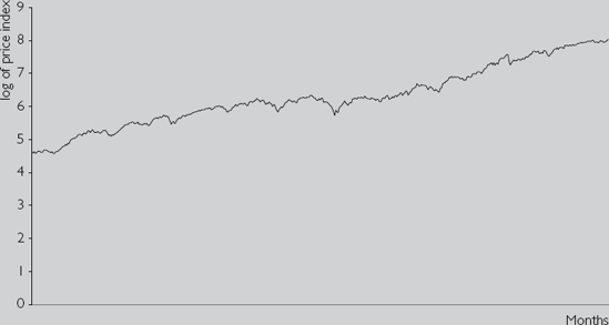
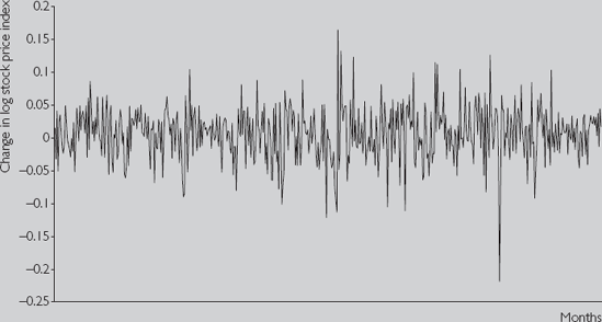
Another property of time series data, not usually present in cross-sectional data, is the existence of correlation across observations. The stock price index today, for example, is highly correlated with its value last month.[48] In the jargon of Chapter 8, the variable "stock price" is correlated with the variable "stock price lagged one period". In fact, if we calculate the correlation between the stock price and lagged stock price we obtain 0.999044. Yet, if we calculate the correlation between the change in the stock price index and the change in the stock price index lagged once, we obtain 0.039. These findings make intuitive sense. Stock markets change only slowly over time; even in bear markets they rarely fall by more than a few percent per month. Consequently, this month's stock price tends to be quite similar to last month's and both are highly correlated. Yet, the return on the stock market is more erratic. This month's and last month's return can be quite different, as reflected in the near-zero correlation between them.
Figures 9.1 and 9.2 and the correlation results discussed in the previous paragraph were calculated using a stock market index. But other financial time series exhibit very similar types of behavior. Y, in other words, tends to exhibit trend behavior and to be highly correlated over time, but ΔY tends to the opposite, i.e. exhibits no trend behavior and is not highly correlated over time. These properties are quite important to regression modeling with time series variables as they relate closely to the issue of nonstationarity. Appropriately, we will spend the rest of this chapter developing formal tools and models for dealing with them.
The correlations discussed above are simple examples of autocorrelations (i.e. correlations involving a variable and a lag of itself). The autocorrelation function is a common tool used by researchers to understand the properties of a time series. Based on the material in the "Aside on lagged variables" and the "Aside on notation" from Chapter 8, we will use expressions like "the correlation between Y and lagged Y". We denote this as r1.
In general, we may be interested in the correlation between Y and Y lagged p periods. For instance, our stock market data is observed monthly, so the correlation between Y and Y lagged p = 12 periods is the correlation between the stock price now and the stock price a year ago (i.e. a year is 12 months). We will denote this correlation by rp and refer to it as "the autocorrelation at lag p". The autocorrelation function treats rp as a function of p (i.e. it calculates rp for p = 1, ..., P). P is the maximum lag length considered and is typically chosen to be quite large (e.g. P = 12 for monthly data). The autocorrelation function is one of the most commonly used tools in univariate time series analysis, precisely because it reveals quite a bit of information about the series.
rp is the correlation between a variable (say, Y) and Y lagged p periods. In our discussion of r1 we noted Y1 lagged one period was Y0, which did not exist. For this reason, we used data from t = 2, ..., T to define lagged Y and calculate r1. An even more extreme form of the problem occurs in the calculation of rp. Consider creating a new variable W which has observations Wt = Yt for t = p + 1, ..., T and a new variable Z which has observations Zt = Yt−p for t = p + 1, ..., T. The correlation between W (i.e. Y) and Z (i.e. Y lagged p periods) is rp. Note that each of the new variables contains T – p observations. So when we calculate rp we are implicitly "throwing away" the first p observations. If we considered extremely long lags, we would be calculating autocorrelations with very few observations. In the extreme case, if we set p = T we have no observations left to use. This is a jus-tification for not letting p get too big. The issues raised in this paragraph are very similar to those raised in distributed lag models (see Chapter 8, "Aside on lagged variables").
The autocorrelation function involves autocorrelations with different lag lengths. In theory, we can use data from t = 2, ..., T to calculate r1; data from t = 3, ..., T to calculate r2; etc., ending with data from t = P + 1, ..., T to calculate rp. But, note that this means that each autocorrelation is calculated with a different number of data points. For this reason, it is standard practice to select a maximum lag (P) and use data from t = P + 1, ..., T for calculating all of the autocorrelations.
The autocorrelation function is a useful tool for summarizing the properties of a time series. Yet, in Chapters 3 and 4, we argued that correlations have their limitations and that regression was therefore a preferable tool. The same reasoning holds here: autocorrelations, in other words, are just correlations, and for this reason it may be desirable to develop more sophisticated models to analyze the relationships between a variable and lags of itself. Many such models have been developed in the statistical literature on univariate time series analysis but the most common model, which can also be interpreted as a regression model, is the so-called autoregressive model. As the name suggests, it is a regression model where the explanatory variables are lags of the dependent variable (i.e. "auto" means "self" and hence an autoregression is a regression of a variable on lags of itself). The word "autoregressive" is usually shortened to "AR".
We begin by discussing the autoregressive model with the explanatory variable being the dependent variable lagged one period. This is called the AR(1) model:
for t = 2, ..., T. It looks exactly like the regression model discussed in previous chapters,[49] except that the explanatory variable is Yt−1. The value of φ in the AR(1) model is closely related to the behavior of the autocorrelation function and to the concept of nonstationarity.
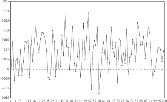
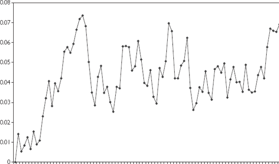
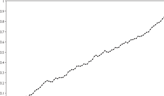
In order to understand the types of behavior characteristic of the AR(1) series, let us artificially simulate three different time series using three different choices for φ : φ = 0, 0.8 and 1. All three series have the same values for a (i.e. α = 0.01) and the same errors. Figures 9.5, 9.6 and 9.7 provide time series plots of the three data sets.
Note that Figure 9.5 (with φ = 0) exhibits random-type fluctuations around an average of about 0.01 (the value of α). In fact, it is very similar to Figure 9.2, which contains a time series plot of stock returns. Figure 9.7 (with φ = 1) exhibits trend behavior and looks very similar to Figure 9.1, which plots the stock price level. Figure 9.6 (with φ = 0.8) exhibits behavior that is somewhere in-between the random fluctuations of Figure 9.5 and the strong trend of Figure 9.7.
Figures 9.5–9.7 illustrate the types of behavior that AR(1) models can capture and show why they are commonly used. For different values of φ, these models can allow for the randomly fluctuating behavior typical of growth rates of many financial time series; for the trend behavior typical of the financial series themselves; or for intermediate cases between these extremes.
Note also that φ = 1 implies the type of trend behavior we have referred to as non-stationary above, while the other values of φ imply stationary behavior. This allows us to provide a formal definition of the concepts of stationarity and nonstationarity, at least for the AR(1) model: For the AR(1) model, we can say that Y is stationary if |φ| < 1 and is nonstationary if φ = 1. The other possibility, |φ| > 1, is rarely considered in finance. The latter possibility implies that the time series is exhibiting explosive behavior over time. Since such explosive behavior is only observed in unusual cases, it is of little empirical relevance and we shall not discuss it here. Mathematical intuition for the properties of the AR(1) model and how it relates to the issue of nonstationarity is given in Appendix 9.1.
Above we introduced the terms "nonstationary" and "stationary" without providing any formal definition (except for the AR(1) model). As we shall see, the distinction between stationary and nonstationary time series is an extremely important one. To formally define these concepts requires that we get into statistical issues that are beyond the scope of this book. But we provide some general intuition for these concepts below.
Formally, "nonstationary" merely means "anything that is not stationary". Economists usually focus on the one particular type of nonstationarity that seems to be present in many financial time series: unit root nonstationarity. We will generalize this concept later, but at this stage it is useful to think of a unit root as implying φ = 1 in the AR(1) model. Following are different ways of thinking about whether a time series variable, Y, is stationary or has a unit root:
In the AR(1) model, if φ = 1, then Y has a unit root. If |φ| < 1 then Y is stationary.
If Y has a unit root then its autocorrelations will be near one and will not drop much as lag length increases.
If Y has a unit root, then it will have a long memory. Stationary time series do not have long memory.
If Y has a unit root then the series will exhibit trend behavior (especially if α is non-zero).
If Y has a unit root, then ΔY will be stationary. For this reason, series with unit roots are often referred to as difference stationary series.
The final point can be seen most clearly by subtracting Yt−1 from both sides of the equation in the AR(1) model, yielding:
where ρ = φ – 1. Note that, if φ = 1, then ρ = 0 and the previous equation can be written solely in terms of ΔYt, implying that ΔYt fluctuates randomly around α. For future reference, note that we can test for ρ = 0 to see if a series has a unit root. Furthermore, a time series will be stationary if −1 < φ < 1 which is equivalent to −2 < ρ < 0. We will refer to this as the stationarity condition.
By way of providing more intuition (and jargon!) for the AR(1) model, let us consider the case where φ = 1 (or, equivalently, ρ = 0). In this case we can write the AR(1) model as:
This is referred to as the random walk model. More precisely, the random walk model has no intercept (i.e. α = 0), while the preceding equation is referred to as a random walk with drift. The presence of the intercept allows for changes in variables to be, on average, non-zero. So, for instance, if Y is (the log of) a stock price of a particular company then the random walk with drift model can be written as:
Since the left-hand of this equation is the stock return (exclusive of dividends), then the model says stock returns are equal to α (e.g. a benchmark return relevant for this company taking into account its risk, etc.) plus a random error.
In the random walk model, since φ = 1, Y has a unit root and is nonstationary. This model is commonly thought to hold for phenomena like stock prices, a point we will elaborate on next.
We have argued above that the AR(1) model can be interpreted as a simple regression model where last period's Y is the explanatory variable. However, it is possible that more lags of Y should be included as explanatory variables. This can be done by extending the AR(1) model to the autoregressive of order p, AR(p), model:
for t = p + 1, ..., T. We will not discuss the properties of this model, other than to note that they are similar to the AR(1) model but are more general in nature. That is, this model can generate the trend behavior typical of financial time series and the randomly fluctuating behavior typical of their growth rates.
In discussing unit root behavior it is convenient to subtract Yt−1 from both sides of the previous equation. With some rearranging[51] we obtain:
where the coefficients in this regression, ρ, γ1, ..., γp−1 are simple functions of φ1,..., φp. For instance, ρ = φ1 + ...+ φp – 1. Note that this is identical to the AR(p) model, but is just written differently. Hence we refer to both previous equations as AR(p) models. In case you are wondering where the Yt−p term from the first equation went to in the second, note that it appears in the second equation in the ΔYt−p+1 term (i.e. ΔYt−p+1 = Yt−p+1 – Yt−p). Note also that both variants have the same number of coefficients, p + 1 (i.e. the first variant has α, φ1, ..., φp while the second variant has α, ρ, γ1, ..., γp−1). However, in the second variant the AR(p) model has last coefficient γp−1. Don't let this confuse you, it is just a consequence of the way we have rearranged the coefficients in the original specification.
The key points to note here are that the above equation is still in the form of a regression model; and ρ = 0 implies that the AR(p) time series Y contains a unit root; if −2 < ρ < 0, then the series is stationary. Looking at the previous equation with ρ = 0 clarifies an important way of thinking about unit root series which we have highlighted previously: if a time series contains a unit root then a regression model involving only ΔY is appropriate (i.e. if ρ = 0 then the term Yt−1 will drop out of the equation and only terms involving ΔY or its lags appear in the regression). It is common jargon to say that "if a unit root is present, then the data can be differenced to induce stationarity".
As we will discuss in the next chapter, with the exception of a case called cointegration, we do not want to include unit root variables in regression models. This suggests that, if a unit root in Y is present, we will want to difference it and use ΔY. In order to do so, we must know first if Y has a unit root. In the past, we have emphasized that unit root series exhibit trend behavior. Does this mean that we can simply examine time series plots of Y for such trending to determine if it indeed has a unit root? The answer is no. To explain why, let us introduce another model.
We showed previously that many financial time series contain trends and that AR models with unit roots also imply trend behavior. However, there are other models that also imply trend behavior. Imagine that Figure 9.1 (or Figure 9.7) is an XY-plot where the X-axis is labeled time, and that we want to build a regression model using this data. You might be tempted to fit the following regression line:
where the coefficient on the explanatory variable, time, is labeled δ to distinguish it from the φ in the AR(1) model. Note that you can interpret the previous regression as involving the variable Y and another variable with observations 1, 2, 3, 4, ..., T. This is another regression model which yields trend behavior. To introduce some jargon, the term δt is referred to as a deterministic trend since it is an exact (i.e. deterministic) function of time. In contrast, unit root series contain a so-called stochastic trend (justification for the term "stochastic trend" is given in Appendix 9.1).
We can even combine this model with the AR(1) model to obtain:
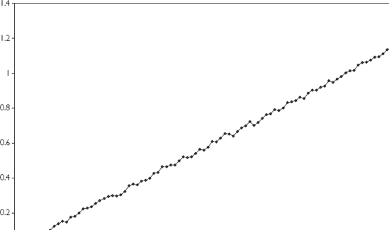
Figure 9.8 is a time series plot of artificial data generated from the previous model with α = 0, φ = 0.2 and δ = 0.01. Note that this series is stationary since |φ| < 1. Yet, Figure 9.8 looks much like Figure 9.7 (or Figure 9.1). Stationary models with a deterministic trend can yield time series plots that closely resemble those from non-stationary models having a stochastic trend. Thus, you should remember that looking at time series plots alone is not enough to tell whether a series has a unit root.
The discussion in the previous paragraph motivates jargon that we will use and introduce in the context of the following summary:
The nonstationary time series variables on which we focus are those containing a unit root. These series contain a stochastic trend. But if we difference these time series, the resulting time series will be stationary. For this reason, they are also called difference stationary.
The stationary time series on which we focus have −2 < ρ < 0 in the AR(p) model. However, these series can exhibit trend behavior through the incorporation of a deterministic trend. In this case, they are referred to as trend stationary.
If we add a deterministic trend to the AR(p) model, we obtain a very general model that is commonly used in univariate time series analysis:
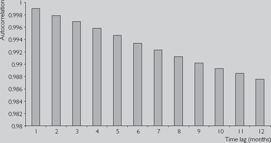
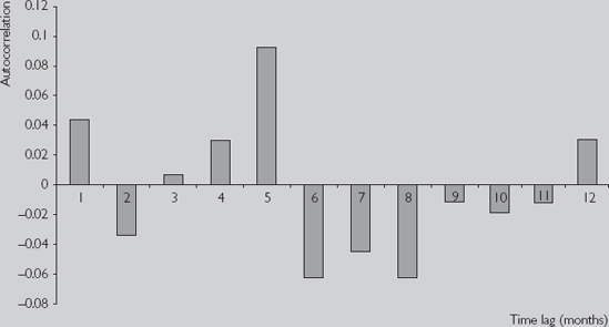
We refer to the above as the AR(p) with deterministic trend model and use it later. You may wonder why we don't just use the original AR(p) specification introduced at the beginning of this section (i.e. the one where the explanatory variables are Yt-1, ..., Yt−p). There are two reasons. First, we are going to test for a unit root. With the present specification, this is simply a test of ρ = 0. Testing for whether regression coefficients are zero is a topic which we have learned previously (refer to Chapter 5). With the original AR(p) model, testing for a unit root is more complicated. Second, Yt−1, Yt−2, ..., Yt−p are often highly correlated with each other (see the autocorrelation function in Figure 9.3). If we were to use them as explanatory variables in our regression we might run into serious multicollinearity problems (see Chapter 6). However, in the present model we use Yt−1, ΔYt−1, ..., ΔYt−p+1 as explanatory variables, which tend not to be highly correlated (see Figure 9.4), thereby avoiding the problem.
Table 9.2. AR(4) with deterministic trend model.
Coefficient | Standard error | t-stat | P-value | Lower 95% | Upper 95% | |
|---|---|---|---|---|---|---|
Intercept | 0.082 | 0.039 | 2.074 | 0.039 | 0.004 | 0.161 |
Yt−1 | −0.016 | 0.008 | −1.942 | 0.053 | −0.033 | 0.0002 |
ΔYt−1 | 0.051 | 0.044 | 1.169 | 0.243 | −0.035 | 0.138 |
ΔYt−2 | −0.027 | 0.044 | −0.623 | 0.534 | −0.114 | 0.059 |
ΔYt−3 | 0.015 | 0.044 | 0.344 | 0.731 | −0.071 | 0.101 |
time | 1E – 4 | 5E – 5 | 1.979 | 0.048 | 7E – 7 | 0.0002 |
In Chapters 5 and 6, we described how to test whether regression coefficients were equal to zero. These techniques can be used in the AR(p) with deterministic trend model (i.e. if you wish to omit explanatory variables whose coefficients are not significantly different from zero). In particular, testing is usually done to help choose lag length (p) and to decide whether the series has a unit root. In fact, it is common to first test to select lag length (using hypothesis tests as described in Chapter 8), and then test for a unit root.
However, there is one important complication that occurs in the AR(p) model that was not present in earlier chapters. To understand it, let us divide the coefficients in the model into two groups: (1) α, γ1, ..., γp−1, and Δ, and (2) ρ. In other words, we consider hypothesis tests involving ρ separately from those involving the other coefficients.
Many sophisticated statistical criteria and testing methods exist to determine the appropriate lag length in an AR(p) model. Nonetheless, simply looking at the t-statistics or P-values in regression outputs can be quite informative. For instance, an examination of Table 9.2 reveals that the P-values associated with the coefficients on the lagged ΔY terms are insignificant, and that they may be deleted from the regression (i.e. the P-values are greater than 0.05). Alternatively, a more common route is to proceed sequentially, as we did in Chapter 8; that is, to choose a maximum lag length, pmax, and then sequentially drop lag lengths if the relevant coefficients are insignificant.
More specifically, begin with an AR(pmax). If the pmaxth lag is insignificant, we reduce the model to an AR(pmax – 1). If the (pmax – 1)th lag is insignificant in the AR(pmax – 1) then drop it and use an AR(pmax – 2), etc. Generally, you should start with a fairly large choice for pmax.
In the AR(p) with deterministic trend model we also have to worry about testing whether δ = 0. This can be accomplished in the standard way by checking whether its P-value is less than the level of significance (e.g. 0.05). This test can be done at any stage, but it is common to carry it out after following the sequential procedure for choosing p.
A short summary of this testing strategy is outlined below:
Step 1. Choose the maximum lag length, pmax, that seems reasonable to you.
Step 2. Estimate using OLS the AR(pmax) with deterministic trend model:
If the P-value for testing γpmax−1 = 0 is less than the significance level you choose (e.g. 0.05) then go to Step 5, using pmax as lag length. Otherwise go on to the next step.
Step 3. Estimate the AR(pmax – 1) model:
If the P-value for testing γpmax−2 = 0 is less than the significance level you choose (e.g. 0.05) then go to Step 5, using pmax – 1 as lag length. Otherwise go on to the next step.
Step 4. Repeatedly estimate lower order AR models until you find an AR(p) model where γp−1 is statistically significant (or you run out of lags).
Step 5. Now test for whether the deterministic trend should be omitted; that is, if the P-value for testing δ = 0 is greater than the significance level you choose then drop the deterministic trend variable.
Table 9.3 shows the table of results you might report in a paper or empirical project, including a brief but coherent explanation of the strategy that you used to arrive at this final specification.
These results lead us to the next, most important, testing question: does Y contain a unit root? Remember that, if ρ = 0, then Y contains a unit root. In this case, the series must be differenced in the regression model (i.e. it is difference stationary). You may think that you can simply test ρ = 0 in the same manner as you tested the significance of the other coefficients. For instance, you might think that by comparing the P-value to a significance level (e.g. 0.05), you can test for whether ρ = 0. SUCH A STRATEGY IS INCORRECT! In hypothesis testing, ρ is different from other coefficients and, thus, we must treat it differently.
To fully understand why you cannot carry out a unit root test of ρ = 0 in the same manner as we would test other coefficients requires that you have knowledge of statistics beyond that covered in this book. Suffice it to note here that most regression packages like Excel implicitly assume that all of the variables in the model are stationary when they calculate P-values. If the explanatory variable Yt−1 is nonstation-ary, its P-value will be incorrect. A correct way of testing for a unit root has been developed by two statisticians named Dickey and Fuller and is known as the Dickey—Fuller test.[52] They recommend using the t-statistic for testing ρ = 0, but correcting the P-value.
We can motivate the Dickey–Fuller test in terms of the following: in Chapter 5, we said that testing could be done by comparing a test statistic (here the t-stat) to a critical value to determine whether the former was either "small" (in which case the hypothesis was accepted) or "large" (in which case the hypothesis was rejected). In the standard (stationary) case, the critical values are taken from statistical tables of the Student-t distribution. Dickey and Fuller demonstrated that in the unit root case, this is incorrect. They calculated the correct statistical tables from which to take critical values.
The previous paragraphs were meant to motivate why the standard testing procedure was incorrect. Admittedly, they are not very helpful in telling you what to do in practice. If you are going to work extensively with time series data, it is worthwhile to either:
Use a computer software package that is more suitable for time series analysis than Excel. Packages such as Stata, E-views, MicroFit or SHAZAM will automatically provide you with correct critical values or P-values for your unit root test. As before, you will reject the unit root if the P-value is less than 0.05 or if the t-stat is greater than the critical value (in an absolute value sense).
Read further in time series econometrics and learn how to use the Dickey–Fuller statistical tables.[53]
However, a rough rule of a thumb can be used that will not lead you too far wrong if your number of observations is moderately large (e.g. T > 50). This approximate rule is given in the following strategy for testing for a unit root:
Use the strategy outlined in Steps 1 to 5 above to estimate the AR(p) with deterministic trend model. Record the t-stat corresponding to ρ (i.e. the t-stat for the coefficient on Yt−1).
If the final version of your model includes a deterministic trend, the Dickey–Fuller critical value is approximately −3.45. If the t-stat on ρ is more negative than −3.45, reject the unit root hypothesis and conclude that the series is stationary. Otherwise, conclude that the series has a unit root.
If the final version of your model does not include a deterministic trend, the Dickey–Fuller critical value is approximately −2.89. If the t-stat on ρ is more negative than −2.89, reject the unit root hypothesis and conclude that the series is stationary. Otherwise, conclude that the series has a unit root.[54]
In the previous example, the final version of the AR(p) model did not include a deterministic trend. The t-stat on ρ is −0.063, which is not more negative than −2.89. Hence we can accept the hypothesis that NYSE stock prices contain a unit root and are, in fact, a random walk. Be careful using this crude rule of thumb when your t-stat is close to the critical values listed here.
Some words of warning about unit root testing: The Dickey–Fuller test exhibits what statisticians refer to as low power. In other words, the test can make the mistake of finding a unit root even when none exists. Intuitively, trend stationary series can look a lot like unit root series (compare Figures 9.7 and 9.8) and it can be quite hard to tell them apart. Furthermore, other kinds of time series models can also appear to exhibit unit root behavior, when in actuality they do not have unit roots. A prime example is the time series model characterized by abrupt changes or breaks. These structural breaks can occur in time series models, and can be precipitated by events such as wars or crises in supply (e.g. the OPEC oil embargo). Stock prices can exhibit structural breaks due to market crashes; and commodity prices, due to droughts and other natural disasters. All in all, structural breaks are potentially a worry for many types of time series data and some caution needs to be taken when interpreting the results of Dickey–Fuller tests. There are many other tests for a unit root. To explain these would require a long technical digression which would distract from the main focus of this book. However, depending on which software package you have available, a little bit of extra study should enable you to use them in practice. Remember the structure of any hypothesis testing procedure involves your knowing the hypothesis being tested (here the unit root hypothesis) as well as a P-value (or a test statistic with critical value to compare it to). Many software packages provide these automatically. For instance, Stata allows you to do another popular unit root test called the Phillips–Perron test (as well as others) in this manner.
Many financial time series exhibit trend behavior, while their differences do not exhibit such behavior.
The autocorrelation function is a common tool for summarizing the relationship between a variable and lags of itself.
Autoregressive models are regression models used for working with time series variables. Such models can be written in two ways: one with Yt as the dependent variable, the other with ΔYt as the dependent variable.
The distinction between stationary and nonstationary models is a crucial one.
Series with unit roots are the most common type of nonstationary series considered in financial research.
If Yt has a unit root then the AR(p) model with ΔYt as the dependent variable can be estimated using OLS. Standard statistical results hold for all coefficients except the coefficient on Yt−1.[55]
The Dickey–Fuller test is a test for the presence of a unit root. It involves testing whether the coefficient on Yt−1 is equal to zero (in the AR(p) model with ΔYt being the dependent variable). Software packages such as Excel do not print out the correct P-value for this test.
Mathematical insight into the properties of the AR(1) model can be gained by writing it in a different way. For simplicity, we will set α = 0 in order to focus on the role that lagged Y plays. Note that the AR(1) model will hold at any point in time so we can lag the whole AR(1) equation given in the body of the chapter and write:
If we substitute this expression for Yt−1 into the original AR(1) model we obtain:
Note that the previous expression depends on Yt−2, but we can write:
and substitute this expression for Yt−2 in the other equation. If this procedure is repeated we end up with an alternative expression for the AR(1) model:

This expression looks complicated, but we can consider two special cases as a means of understanding its implications. In the first of these we assume φ = 1 and the previous equation reduces to:

The important point to note about the two terms on the right hand side of the previous equation is that they illustrate a long memory property; the value of the time series starts at Y1, which always enters the expression for Yt, even if t becomes very large. That is, the time series "never forgets" where it started from. It also "never forgets" past errors (e.g. e1 always enters the above formula for Yt even if t gets very large). It can be shown that the trending behavior of this model arises as a result of the second term, which says that current Y contains the sum of all past errors. Statisticians view these errors as random or "stochastic" and this model is often referred to as containing a stochastic trend. This is a key property of nonstationary series.
A second special case stands in contrast to the properties described above. If we suppose |φ| < 1, we can see that φt−1 will be decreasing as t increases (e.g. if φ = 0.5, then φ2 = 0.25, φ10 = 0.001 and φ100 = 7.89 × 10⁻³¹, etc.). The influence of Y1 and past errors on Yt will gradually lessen as t increases and Y slowly "forgets the past". Y will not exhibit the long memory property we observed for the case where φ = 1. This is a key property of stationary series.
[46] Details about logarithms are discussed in Chapters 1, 2 and 4 (see especially the discussion on Nonlinearity in Regression). This footnote is intended to refresh your memory of this material. It is common to take the natural logarithm of the time series if it seems to be growing over time. If a series, Y, is growing at a roughly constant rate, then the time series plot of ln(Y) will approximate a straight line. In this common case, ln(Y) will generally be well-behaved. Note also that in regressions of logged variables, the coefficients can be interpreted as elasticities. It can also be shown that ln(Yt) – ln(Yt−1) is approximately equal to the percentage change in Y between periods t – 1 and t.
For all these reasons, it is often convenient to work with logged series. Note that this log transformation is so common that many reports and papers will initially explain that the variables are logged, but thereafter drop the explicit mentioning of the log transformation. For instance, an author might refer to "the natural log of wealth" as "wealth" for brevity. We will follow this tradition in the examples in this book.
[47] Since Y0 is not known, ΔYt runs from t = 2, ..., T rather than from t = 1, ..., T. We focus on the empirically useful case of first-differencing but we can define higher orders of differencing. For instance, the second difference of Yt is defined as: Δ2Yt = ΔYt – ΔYt−1.
[48] Put another way, if you knew what the stock price index was today (let's say, in January it is 2,000), you could make a pretty good guess about roughly what it would be next month. That is, it might go up or down a couple percentage points to 2,100 or 1,900, but it is highly unlikely to be, say, 100 or 5,000. This ability to predict well is evidence of high correlation.
[49] It is common practice to use Greek letters to indicate coefficients in regression models. We can, of course, use any Greek symbol we want to denote the slope coefficient in a regression. Here we have called it φ rather than β. We will reserve β (perhaps with a subscript) to indicate coefficients relating to the explanatory variable X.
[50] Some statistical problems arise with OLS estimation of this model, if the model is non-stationary or nearly so (i.e. φ is close to one or, equivalently, ρ is close to zero). Nevertheless, OLS is still a very common estimation method for AR models (especially if φ is not that close to 1), so you will probably not go far wrong through sticking with OLS when working with AR models. If you take courses in financial econometrics or time series statistics in the future, you will undoubtedly learn about other estimators.
[51] Each step in the derivation of this equation involves only simple algebra (e.g. subtracting the same thing from both sides of the equation, etc.). However, there are many steps involved and the derivation of this equation is a bit messy.
[52] Some authors use the term "Dickey—Fuller test" for testing for ρ = 0 in the AR(1) model and use the term "Augmented Dickey—Fuller test" for testing in the AR(p) model (i.e. the basic unit root test is "augmented" with extra lags).
[53] Undergraduate Econometrics by Carter Hill, William Griffiths and George Judge (second edition, John Wiley & Sons, Ltd, 2000), Chapter 16 is a good place to start.
[54] Formally, −3.45 and −2.89 are the critical values for T = 100 using a 5% level of significance. Critical values for values of T between 50 and infinity are within 0.05 of these values.
[55] Formally, standard hypothesis tests can be conducted on coefficients on stationary variables.

