By applying formatting, you can change the way numbers display. For example, you can use Excel's formatting options to tell Excel you want to separate thousands or show decimal places. Formatting makes your data easier to read and helps you conform to company, country, or industry standards. Excel provides a variety of options for formatting numbers.
When you type numbers into a cell, in most instances they appear in the format you type them. However, if the number has decimal places and is too long to fit in the cell, Excel rounds the number. If the number is longer than 12 digits, Excel displays the number in scientific notation. If the number has leading or trailing zeros, Excel drops the zeros. For example, Excel displays both 0123 and 123.00 as 123.
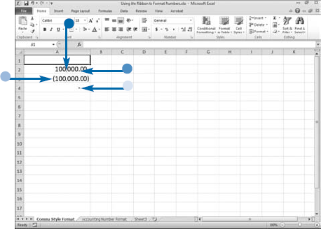
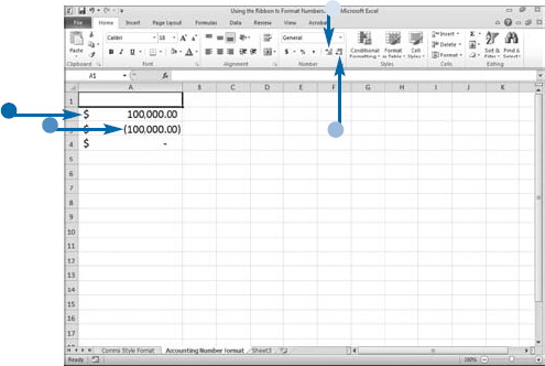
The Number group on the Home tab has several buttons you can use to format numbers quickly. If you choose Comma Style, Excel separates the thousands with a comma, adds two decimal places, displays negative numbers in parentheses, and represents zeros with a dash (−).
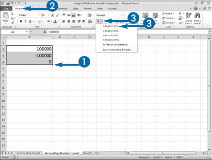
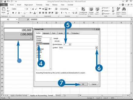
The Accounting Number Format field has several currency formats you can choose from, including the United States currency format, the United Kingdom currency format, and the Euro currency format. For example, if you choose the United States currency format, Excel adds a dollar sign and aligns it with the left side of the cell, adds two decimal places, and displays negative numbers in parentheses. You can click the Increase Decimal or Decrease Decimal buttons to increase or decrease the number of decimal places that appear.
Using the Ribbon to Format Numbers


Excel separates the thousands.
Excel adds two decimal places.
Negative numbers appear in parentheses.
Zeros are represented by a dash.
Apply It
You can use the Number Format field to apply a number format quickly. When you click the down arrow (
Click Number to apply the Number format. The Number format does not display a currency symbol and does not separate thousands, but it does display two decimal places, zeros as 0.00, and negative numbers with a negative sign (–).
If you want to display a number as currency, choose either the Accounting number format or the Currency number format. The Accounting number format aligns the currency symbol with the left side of the cell, displays two decimal places, separates thousands, displays zeros as dashes, and display negative number in parentheses. The Currency format places the currency symbol immediately before the first digit, displays two decimal places, separates thousands, and displays negative numbers with a negative sign (–).
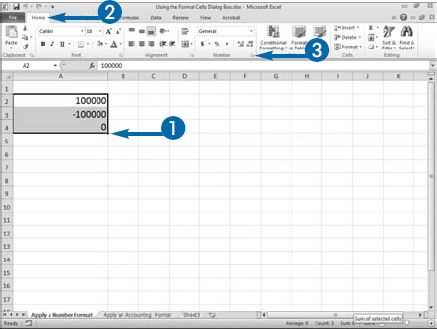
As an alternative to using the Ribbon, you can use the Format Cells dialog box to format cells. The Format Cells dialog box lets you specify how each number is formatted. The General format option is the default format. Generally, it displays numbers exactly as you type them. However, if the number has decimal places and is too long to fit in the cell, Excel rounds the number. If the number is longer than 12 digits, Excel displays the number in scientific notation. If the number has leading or trailing zeros, Excel drops the zeros. If you have changed a number's format and want to return to the original format, choose the General format.
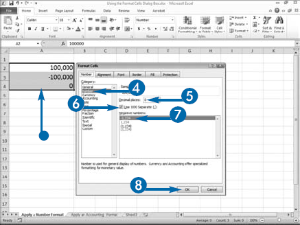
In the Format Cell dialog box you can use Number Format options to set the number of decimal places, specify whether a number should display a thousands separator, and specify how to display negative numbers. You can choose from four formats for negative numbers: preceded by a negative sign (–), in red, in parentheses, or in red and in parentheses.
The Currency format offers you the same options as the Number format except you can choose to display a currency symbol. The currency symbol you choose determines the options you have for displaying negative numbers. If you choose the dollar sign ($), thousands are separated by commas by default.
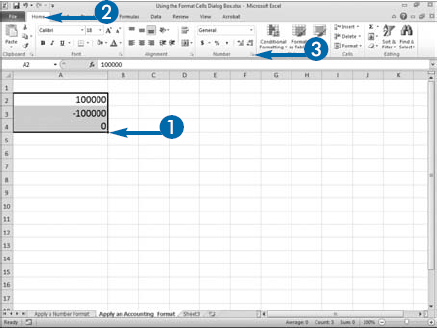
Excel designed the Accounting format to comply with accounting standards. When using the Accounting format, if you choose a currency symbol, the currency symbol aligns with the left side of the cell, decimal points are aligned, a dash (–) displays instead of a zero, and negative numbers display in parentheses.
In Excel, dates and times are numbers. All dates are whole numbers and all times are decimal fractions. By default, Excel for Windows uses a 1900 date system. January 1, 1900, is represented by the number 1; January 2, 1900, is represented by the number 2; January 3, 1900, is represented by the number 3; and every date thereafter is represented by the next sequential number. Times are represented by decimal fractions that range from .0 to .99999. The decimal fraction .0 represents 12:00:00 AM; the decimal fraction .5 represents 12:00:00 PM; and the decimal fraction .99999 represents 11:59:59 PM.
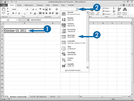
Formats turn these whole numbers and decimal fractions into recognizable dates and times. When you make a cell entry, if Excel recognizes it as a date or a time, it automatically assigns a format. To see the date's whole number or the time's decimal fraction, change the format to the General format. If you want to change the current format of a date or time to another format, you can choose one of the date or time options from the Number Format menu or you can use the Format Cells dialog box.
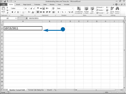
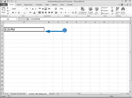
When using the Number Format menu to format Date and Times, the Short Date option formats October 15, 2011, as 10/15/2011; the Long Date option formats it as Saturday, October 15, 2011; and the Time option formats 3:15 p.m. as 3:15:00 PM.
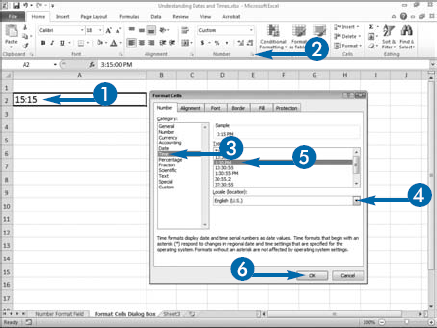
Countries vary in the way they format dates and times. Hence, the Format Cells dialog box provides a variety of ways you can format dates and times based on locale. For example, if you choose English (U.S.) as the locale, Excel provides more then fifteen ways you can format a date.
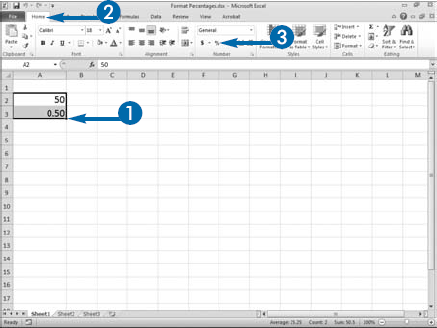
To format a number as a percent, apply the Percentage format. When you apply the Percentage format to an existing number, Excel takes the number, multiplies it by 100, and adds a percent sign. For example, if you apply a Percentage format to 50, you get 5000%. Use this formula to calculate a percentage: amount/total amount = percentage. For 50 out of 100 the calculation is 50/100 = .50; when you apply the Percentage format, you get 50%.
You can preformat a cell by applying a format to the cell before you make an entry. If you preformat, Excel handles percentages differently. If you enter a whole number, Excel converts the whole number to a percent. If you enter a decimal, Excel multiplies the decimal by 100. Both 50 and .50 are interpreted as 50%.
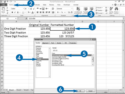
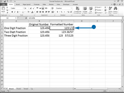
You can format numbers as one-digit, two-digit, or three-digit fractions. When you format a number as a one-digit fraction, Excel rounds the number to the nearest single-digit fraction value; when you format a number as a two-digit fraction, Excel rounds the number to the nearest two-digit fraction value; and when you format a number as a three-digit fraction, Excel rounds the number to the nearest three-digit fraction value. For example, if you format the number 123.456 as a single-digit fraction, you get 123 1/2. If you format it as a two-digit value you get 123 26/57. And, if you format it as a three-digit value you get 123 57/125. You can also format number as halves, quarters, eighths, sixteenths, tenths, and hundredths.
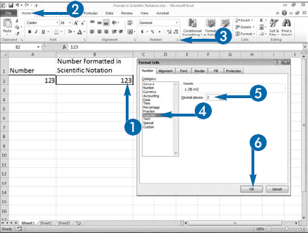
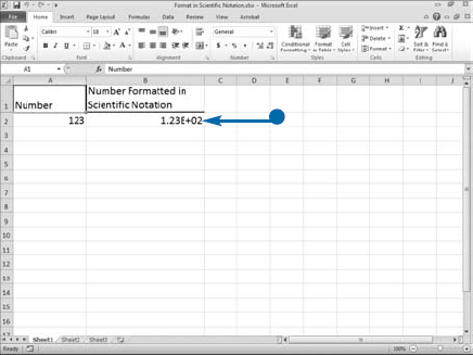
In Excel, you can format numbers in scientific notation. When you are working with extremely large numbers, scientific notation saves space.
The number 1.23E+02 is scientific notation for 123. Scientific notation consists of a number followed by E+n. The E stands for exponent and n is the power to which you need to raise the number 10. To convert a number from scientific notation, multiply the number that precedes the E by 10 and then raise 10 to the power after the plus (+). For example, if you enter the formula =1.23*10^2 into Excel, you get 123. When you format a number in scientific notation, you can specify the number of decimal places you want to keep.
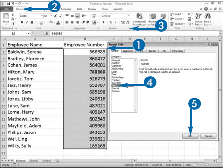
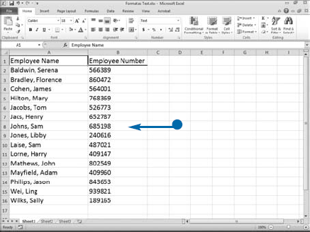
You can use the Text format in the Format Cells dialog box to convert a number to text. Numbers formatted as text are not used in mathematical calculations. Certain numbers — for example, employee numbers — are never used in mathematical calculations and should be formatted as text. If you want to format a number as text as you type it, precede the number with an apostrophe (').
When you enter numbers as text, an error indicator may appear. Excel is checking to see if you entered the number as text by mistake. You should click the Error Indicator button and then click Ignore Error.
By default, numbers are right aligned in the cell and text is left aligned. When you format a number as text, Excel left aligns the number.
Apply It
If you do not want an error indicator to display when you enter a number as text, you can deselect Numbers Formatted as Text or Preceded by an Apostrophe in the Excel Options dialog box. Click the File tab. Click Options. Click Formulas, which is located in the left column. Deselect the Numbers Formatted as Text or Preceded by an Apostrophe option (
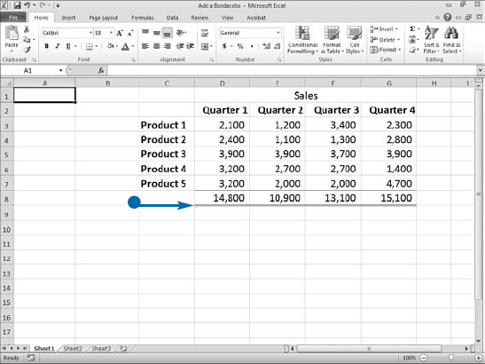
You can highlight important information by adding a border. A border is a set of lines that surround a cell or cell range. You can choose the style, color, and placement of border lines. Adjoining cells share borders. For example, placing a bottom border on cell A1 is the same as placing a top border on cell A2.
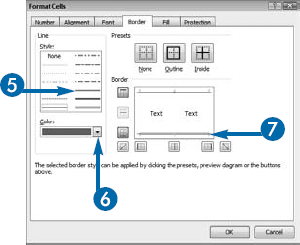
When creating a border, you can choose from the following styles: single line, double line, thick line, or a variety of dotted and dashed lines. You can also choose the color of the line from theme colors, standard colors, or other colors. The border lines can appear on the top of a cell, the bottom of a cell, the left side of a cell, the right side of a cell, diagonally from the top-left corner to the bottom-right corner, or diagonally from the top-right corner to the bottom-left corner, or any combination thereof.
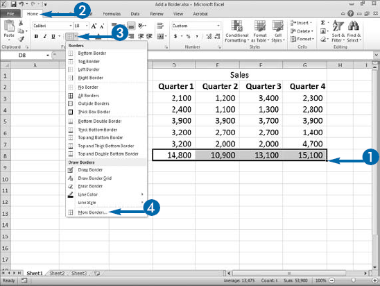
When you click the Border button, Excel provides you with a menu of preset border options. If any one of the border options meets your needs, you can click it to apply it to the selected cells. The Border button displays the last border you applied. If you want to apply that border to another group of cells, simply select the cells and then click the Border button.
You can use the Format Cells dialog box to customize borders. In the Format Cells dialog box, you can use presets to design a border, or you can select the placement of each border. The menu also has options that you can use to draw borders.

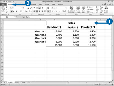
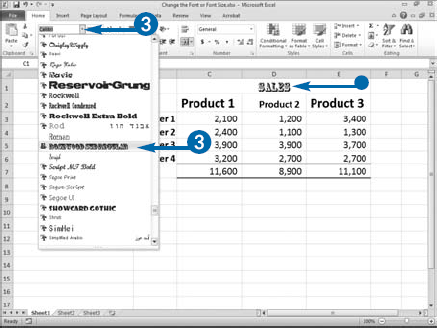
A font is a collection of characters that all have the same basic style. When you open a workbook, if you do not make any changes, Excel uses the default font and font size. You may want to change the font or font size to conform to company standards or to make a portion of your worksheet standout. You can have a variety of fonts and font sizes in a single worksheet. If you select a range of cells, and then move your mouse pointer over each of the options on the Font or Font Size menu, Excel provides you with a preview of how that font or font size will appear if you select it.
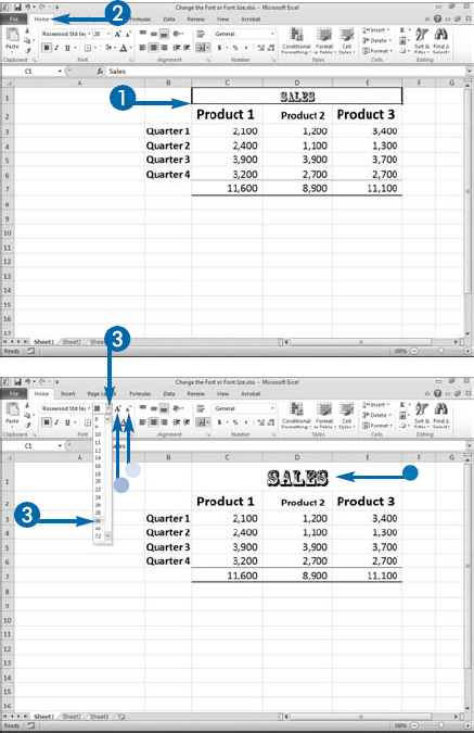
In addition, in the Font group on the Home tab, Excel provides an Increase Font Size button and a Decrease Font Size button. You can click the Increase Font Size button to make the font in selected cells larger. You can click the Decrease Font Size button to make the font in selected cells smaller. You can also enter a font size directly into the Font Size field.
Fonts are measured in points by measuring the longest character in a character set. There are 72 points to an inch. When choosing a font size, you are not limited to the options in the Font Size menu. For example, generally the largest font size in the menu is 72, but you can assign a font size larger than 72.
As you make a font larger, the text and numbers may no longer fit. Text spills over into the next cell and numbers display as pound signs (####). To view the data, make the cell larger or wrap the text.
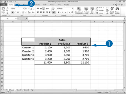
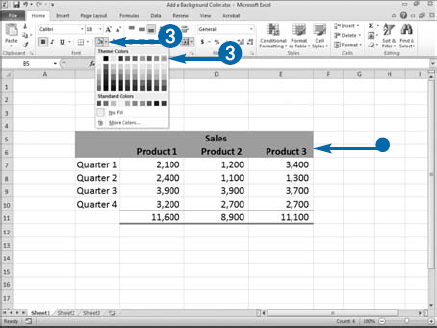
You can make cells stand out by applying a background color, also known as a fill. The fill can be a theme color, a standard color, or any other color.
Theme colors are sets of colors for use throughout a document or document set. Theme colors change when you change the theme. Using theme colors gives documents a consistent look and feel. You can keep the look and feel of your documents consistent across products by using the same theme colors in Word, PowerPoint, and Excel.
You can also use a standard color or you can click More Colors to open the Colors dialog box where you can choose virtually any color. Standard colors and colors from the Color dialog box do not change when you change themes.
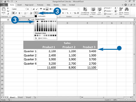
You can make cells stand out by changing the font color. The font color can be a theme color, a standard color, or any other color.
Theme Colors are sets of colors for use throughout a document or document set. If you change the theme, the theme color changes. Standard colors are popular colors. If you change the theme, standard colors do not change.
While you can use any color anywhere, if you have applied a fill, you should combine a light colored font with a dark colored fill or a dark colored font with a light colored fill, so that your text will always be visible in your fill. The first four columns of theme colors are designed for font and fill colors.

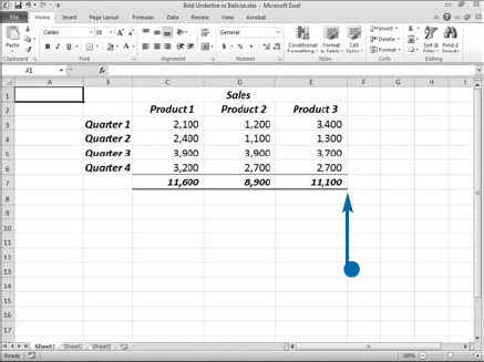
Bolding, underlining, and italicizing are all great ways to make data in your worksheet stand out. For example, you may want to bold your titles, italicize important information, put a single underline under subtotals, and/or put a double underline under totals. Applying these options is as simple as clicking the appropriate button.
If bold, italics, or underlines have been applied to a cell, when you click in the cell the option's button is highlighted on the Ribbon. You can remove the bold, italics, or underlines by clicking the button again. In other words, the Bold, Underline, and Italic buttons are toggle buttons. You click the button once to turn the option on; you click it again to turn the option off.

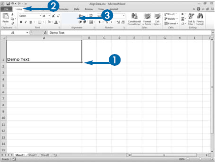
To make your data easier to read, Excel has several buttons you can use to align data in a cell. Click the Align Text Left button to align data with the left side of a cell, click the Align Text Right button to align data with the right side of a cell, or click the Center button to center data in a cell.
Excel also has buttons you can use to place data at the top, bottom, or middle of the cell. Click the Top Align button to align data with the top of the cell, click the Middle Align button to align data with the middle of the cell, and click the Bottom Align button to align data with the bottom of the cell.
By default, the data you enter is horizontal and reads from left to right. If you want to keep your columns narrow, you may want to rotate data so that you can display all of it without making the column wider.
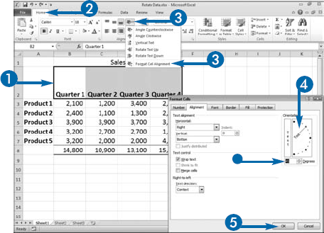
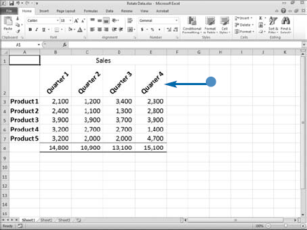
You can use the Orientation menu to rotate data 45 degrees clockwise, 45 degrees counterclockwise, vertically, upward, or downward. You can use the Format Cells dialog box to enter the exact number of degrees you want to rotate data. Use the mouse pointer to tell Excel the angle you want or enter the exact number of degrees directly into the Degrees field. You can enter any number between −90 and 90. Enter a positive number to rotate upward. Enter a negative number to rotate downward.
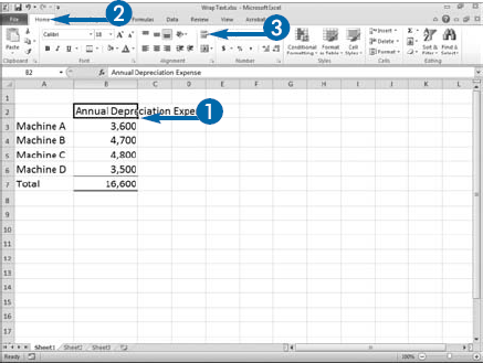
If the text you enter is too long to fit in a single cell, Excel allows the text to spill over into adjacent cells. At that point, the text takes up more that one cell. If you place data in an adjacent cell, Excel cuts off the text in the original cell and, as a result, you cannot see all of it. To rectify this problem, you can use the Excel Wrap Text feature to display the text on multiple lines. The Wrap Text feature increases the height of the cell and then wraps the text in the cell. If you cannot see all the text after performing the wrap text, try increasing the height of the cell manually or reset the row height by using the AutoFit Row Height feature.

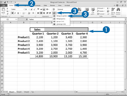
Titles provide a brief summary of your data. You may want to center them over the data they summarize. You can center text within a cell by clicking the Center button. To center text across several cells, click the Merge & Center button. Merge & Center turns a cell range into a single cell and deletes all the data except the data located in the uppermost left corner cell.
When you click the down arrow next to the Merge & Center button, a menu with the following options appears: Merge & Center, Merge Across, Merge Cells, and Unmerge. You can click the Merge & Center option to merge and center rows or columns.
You can click the Merge Across option to merge columns without centering. In languages that read from left to right, the data aligns with the left side of the cell. In languages that read from right to left, the data aligns with the right side of the cell.
You can click the Merge Cells option to merge rows or columns without centering. As with the Merge Across option, the column alignment depends on the language. In languages that read from left to right, the data aligns with the left side of the cell. In languages that read from right to left, the data aligns with the right side of the cell.
When you merge rows, the data aligns with the bottom of the cell. The Unmerge Cells option unmerges cells. You can change the alignment of merged cells. You can also rotate the data.

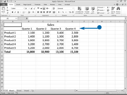
By using Excel's many format options, you can format numbers, text, and cells. A style is a named collection of formats. Styles streamline the work of formatting so that you can apply a consistent set of formats to worksheet elements such as column heads and data values.
Excel divides styles into five categories: Good, Bad, and Neutral; Data and Model; Titles and Headings; Themed Cell Styles; and Number Format. The Good, Bad, and Neutral group and the Data and Model group make it easy for you to categorize cells; the Title and Headings group makes it easy for you to apply headings, the Themed Cell Styles group makes it easy for you to apply a theme color, and the Number Format group makes it easy for you to format numbers.

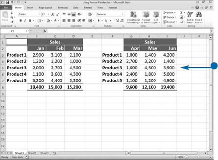
Format Painter can save you time when you need to reapply formats that already exist in your worksheet. You can use Format Painter to apply number, text, cell, shape, or object formats. For example, if you applied a number format to a number and you want another number to have the same format, you can use Format Painter; if you added a background color to a cell and changed the font color and you want another cell to have the same background color and font color, you can use Format Painter; or if you applied a border to a picture and you want another picture to have that same border, you can use Format Painter. Whether you are formatting numbers, text, cells, shapes, or objects, the process is the same.

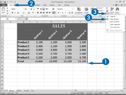
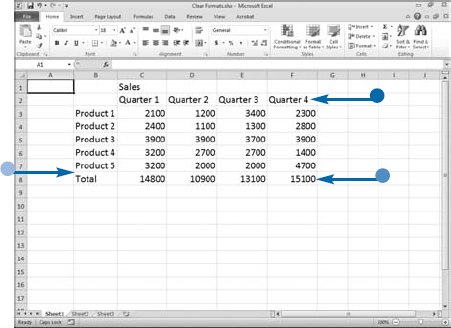
As you have learned by reading this chapter, you can apply a variety formats to Excel data. You can change the font; change the font size; change the font color; add a fill; add a border; apply bold, underlines, and italics; change the orientation of data; change the number format; and more. Once you have applied a format, you can remove the format or you can set the cells back to the default. For example, if you want to remove a border, click No Border on menu that appears when you click the down arrow next to the Border field. If you want to clear all the formats that have been applied to a cell range in a few clicks, use the clear formats option.