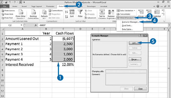
By using the Internal Rate of Return (IRR) function, you can find out how a change in the amount loaned, payment amount, or payment date — or some combination of these factors — affects the interest received. You can type in different amounts at different payment dates to see how different scenarios affect the interest rate.
What-if analysis is a systematic way of finding out how a change in one or more scenarios affects the result. The Scenario Manager lets you vary one or more inputs into any formula or function to see how the result changes.
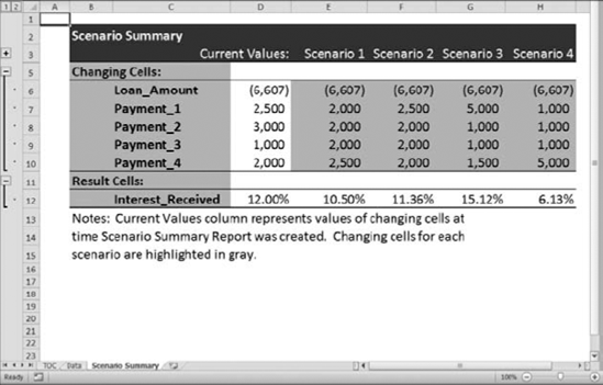
There are two ways to use the scenario manager. You can click a scenario in the Scenario Manager dialog box and then click Show. Excel displays the scenario and the result in your worksheet. When you use this method, Excel changes the values in your worksheet to the values in your scenario. If your original worksheet data is not one of your scenario options, it will be lost. Alternatively, you can create a summary report. A summary report displays each of your scenarios in a different column, in a new worksheet. With a summary report, you can compare scenarios side by side.
The beauty of the Scenario Manager is that it stores a series of values so you can see how each value or combination of values influences the result. You can also present your information as a PivotTable and thereby give yourself all the flexibility a PivotTable offers. To learn more about PivotTables, see Chapter 9.
To create scenarios, you must first enter the values required into a worksheet and type a formula that calculates the answer. The example uses the IRR function.
Perform What-If Analysis


The Scenario Manager dialog box appears.

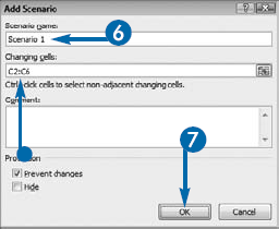
The Add Scenario dialog box appears, showing the cells selected in Step 1.


The Add Scenario dialog box reappears.

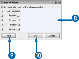

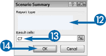
The Scenario Summary dialog box appears.
Alternatively, click a scenario and then click Show to display the scenario in your worksheet.
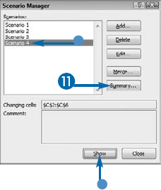


The type of report you requested appears in a new worksheet, displaying how each value affects the result.
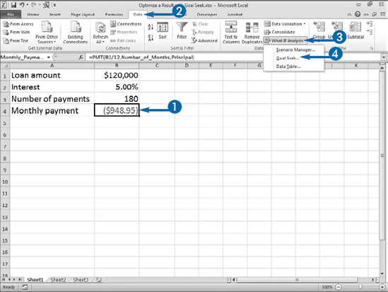
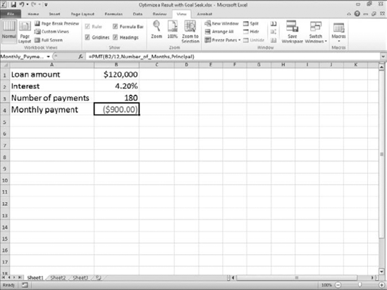
Goal Seek is a powerful tool you can use to find a way to reach your goals. With Goal Seek, you tell Excel which value in your formula you want to change; Excel then adjusts that value to give you the result you want. For example, if you need a loan for a new home and your goal is to make a monthly payment of a specific amount, you can use Goal Seek to show you how you can reach your goal by adjusting one of the loan terms. You can have Goal Seek find the interest rate required to reach your payment goal, given a loan amount and number of payments, find the loan amount required to reach your goal, given an interest rate and number of payments, or find the number of payments required to reach your goal, given an interest rate and loan amount.
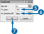
In the Goal Seek dialog box, the Set Cell field tells Excel which cell contains the formula with a value you want to manipulate to achieve your goal. The To Value field tells Excel what your goal is. The By Changing Cell field tells Excel the cell that contains the value you want to change. The cell address you enter in the By Changing Cell field must be included in the formula you reference in the Set Cell field. If you are not getting a result, you can try clicking the Office button, clicking Excel Options, and then clicking Formulas. Then in the Calculations Options area, increase the maximum iterations. This example uses the Payment (PMT) function.
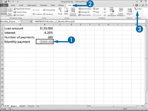
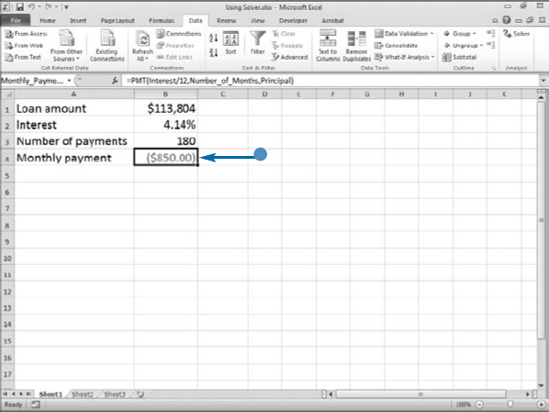
To vary multiple inputs to achieve a specific goal, use Solver. For example, if you want to find out how to adjust both the loan amount and interest rate so that you can reduce a monthly loan payment to from $900.00 to $850.00, you can use Solver.
When using Solver, you must establish a target cell. The target cell is the cell that contains the formula that calculates the goal you want to reach. In this example, it is the cell that contains the payment amount. You must also establish one or more adjustable cells. These are the cells that Solver can change to reach your goal. In this example, the adjustable cells would be the loan amount and the interest rate. The formula in the target cell must directly or indirectly reference the adjustable cells.
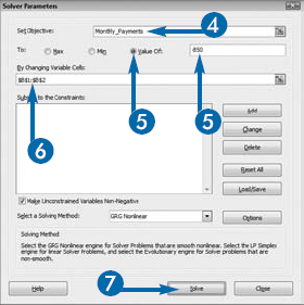
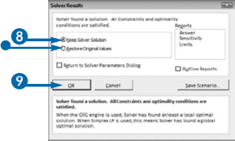
You enter Solver parameters in the Solver Parameters dialog box. In the To field, select Max if you want the target field to be the highest possible value; select Min if you want the target field to be the lowest possible value; and select Value if you want the target field to be a specific value, and then type the value in the field.
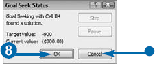
When Solver finds a solution, you can choose either Keep Solver Solution or Restore Original Values. If you choose Keep Solver Solution, Excel permanently changes the worksheet. You cannot undo the changes.
Solver is an add-in. By default, it is not loaded. See Chapter 7 to learn how to load add-ins. Once loaded, Solver appears on the Data tab.
When you need to find out how changing certain values in your formula affects the outcome, you can use a data table. For example, if you want to create a worksheet that shows how different interest rates affect the amount you must pay monthly on a loan, use a data table. With a data table, you can create your worksheet without having to enter the same formula multiple times.
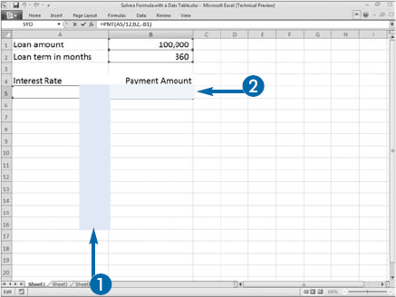
A data table contains at least two columns or two rows. If you use columns, the first column consists of the values you want to substitute into a formula. The first cell of the second column contains the formula you want to use. The formula must reference the first value in the first column. If you are varying interest rates so you can compare loan payments, and the first column (column A) contains the interest rate you want to substitute in the PMT function, the Rate argument must reference column A, as shown in the following formula:
=PMT(A5/PeriodsPerYear, LoanTerm, -LoanAmount)
If you use rows to create your data table, place your substitution values in the first row. Place your formula in the first cell of the second row and reference the first cell of the first row in your formula.
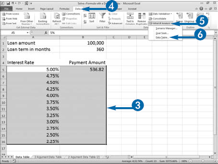
If your data is set up in columns, use the Column input cell field in the Data Table dialog box to tell Excel the location of the cell referenced in your formula. If your data is set up in rows, use the Row input cell field in the Data Table dialog box to tell Excel the location of the cell referenced in your formula.
Solve a Formula with a Data Table
You can also place values in a row.
If your values are in a row, type the formula in the first cell in the row under the values.
A menu appears.
Type the cell reference in this field if you are using rows.
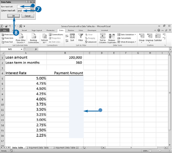
Excel displays the comparison results in the second column of the data table.
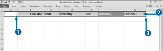
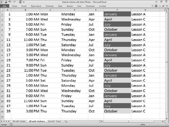
Auto Fill gives you a way to enter data quickly when the data series follows a well-known pattern. For example, you can use Auto Fill to enter the days of the week, the months of the year, or numeric increments of two. All you have to do is enter the initial values and then drag the fill handle. Excel automatically fills the cell with the series. For example, if you want to enter the months of the year, type January, drag the fill handle and as you drag; Excel enters February, March, April, May, and so on. The Fill handle is the small black square in the lower-right corner of the selection area. When you move your mouse pointer over the fill handle, your mouse pointer turns into a cross.
Your fill can consist of numbers, dates, times, months of the year, days of the week, text, or formulas. By default, when filling, Excel also copies the format. For example, if you type Jan in red and then click and drag the fill handle two cells, Excel fills Jan, Feb, Mar using red text. If you type January in a cell with a green background and white text, Excel fills January, February, March using a green background and white text.
After you fill the cells, the AutoFill button appears. Click the button to open a menu that enables you to change the fill. You can copy the initial value to each cell in the fill, fill with formatting only, fill without formatting, or fill with weekdays, months, or years, depending on the type of fill you created.
Extend a Series with Auto Fill
Fill with a Series
Excel fills the cells with a series.
The AutoFill Options button appears.
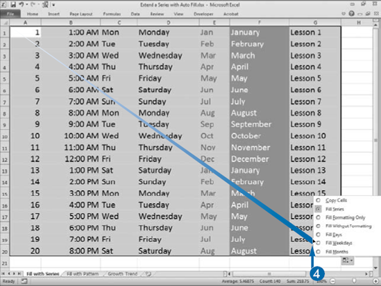
A menu appears.
Use the menu to change the manner in which Excel fills the cells.
Excel fills the cells with the pattern.
Extra
When you release the mouse button after creating a series, the Auto Fill Options button appears. Click the button to view a menu of options. If you want to fill with the days of the week, you can click Fill Days to fill with Sunday through Saturday or Fill Weekdays to fill with Monday through Friday. You can also click the Fill Formatting Only option to change the formatting of the cell without changing the contents. Click the Fill Without Formatting option to change the contents of the filled cells without changing the formatting.
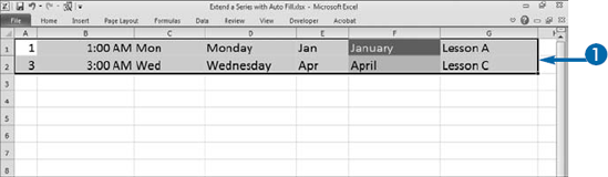
You can fill cells with a growth trend, such as 1, 3, 9, 27 or 2, 4, 8, 16. Type the first two values of the growth trend. Select the values you typed and all the cells you want to fill. Click the Home tab and then click the Fill button (
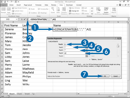
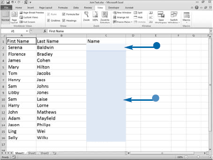
In Excel, you can join text, numbers, and cell references to form a single string of text. For example, if you list first names in one column, and last name in another column, but you need names formatted, last name, comma, first name as in "Smith, John" you can use the you can use the CANCATENATE function to join text so that it is formatted the way you want.
With the CANCATENATE function you can join up to 255 items to form a single string of text. If you need to include a literal value, enclose it in quotes. If you need to include blank spaces, place them between quotes. Separate each value you want to join with a comma.
If you want to do quick calculations without using a formula or function, use a calculator. In Excel, you can place a calculator on the Quick Access Toolbar or on the Ribbon. See Chapter 17 to learn how.
You can use the calculator as you would any electronic calculator. Click a number, choose an operator — such as the plus key (+) to do addition — and then click another number. Press the equal sign key (=) to get a result. Use MS to remember a value, MR to recall it, and MC to clear memory.
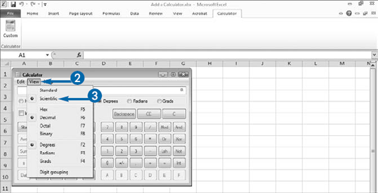
Statistical and mathematical functions are available in the calculator's scientific view when you click View and then Scientific. In this view, you can cube a number, find its square root, compute its log, and more.
Add a Calculator
Note: Before you can use the calculator, you must add it to the Ribbon or to the Quick Access Toolbar. You can find the Calculator button under the Commands not in the Ribbon option in the Choose Commands From field.
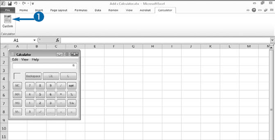
The calculator appears in Standard mode.
The calculator appears in Scientific mode.
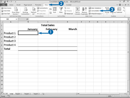
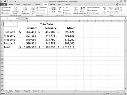
If you keep related data in separate worksheets — or for that matter, separate workbooks — you may eventually want to consolidate the worksheets. For example, if you keep sales information for several regions on separate worksheets, you may want to consolidate the worksheets to find the total sales for all regions. With Excel's Consolidate feature, you can do just that. Excel provides a variety of functions you can use to consolidate, including SUM, COUNT, AVERAGE, MAX, MIN, and PRODUCT.
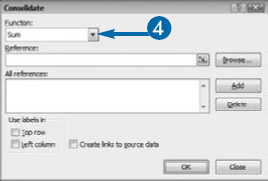
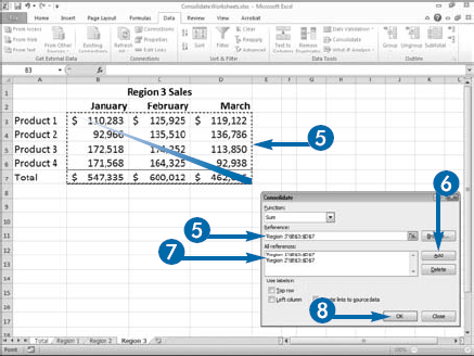
You start the consolidation process by selecting a location for your consolidated data. You can format the cells so the incoming data displays properly. Then select the function you want to use to consolidate your data. The SUM function takes the data from each location you specify and adds it together. You tell Excel the locations of the data you want to consolidate. You can type the range in the Reference field of the Consolidate dialog box or click and drag to select the area. If you type the range, remember to include the worksheet name in single quotes followed by an exclamation point and the range. For example, to refer to the range $B$3:$D$7 on a sheet named Region 1, type 'Region 1'!$B$3:$D$7. Excel takes the data and consolidates it.
If you want to include data from another workbook in your worksheet, open the other workbook. Then in the Consolidate dialog box, place your cursor in the Reference field. Use the View tab to switch windows and choose the other workbook. Once in the workbook, you can click and drag to select the data you want to consolidate.
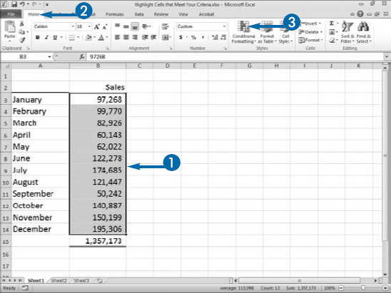
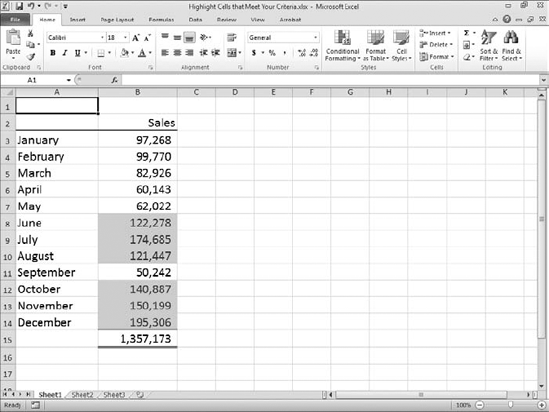
If you want to monitor your data by highlighting a condition, Excel's conditional formatting feature can aid you. For example, if your company offers a bonus when sales exceed $100,000, you can have Excel highlight sales figures whenever cell values in a range of cells are more than $100,000. You can also have Excel highlight a cell when the value is less than, equal to, or between specified values. You can use Excel's conditional formatting feature to monitor numbers, text, and dates. In addition, the conditional formatting feature can check for duplicate values, text that contains a specified series of characters, or a date occurring in a specified time period, such as yesterday, today, tomorrow, or last month.
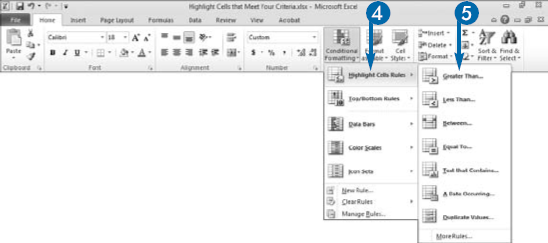
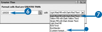
To highlight a condition, you tell Excel the criteria and the format you want to apply if the criteria are met. For example, for sales greater than $100,000, you can choose greater than and enter $100,000 as the value and then choose to display sales that meet that criterion with a light red fill with dark red text, with a yellow fill with dark yellow text, with a green fill with dark green text, with a light red fill, with red text, or with a red border. If none of those formats suit you, you can create a custom format. Your custom format can consist of number formatting, font formatting, border formatting, and/or fill formatting. Excel applies the format you choose to cells that meet the criteria and leaves cells that do not meet the criteria unchanged. You can apply conditional formatting to a cell range, an Excel table, or a PivotTable.
Apply It
You can highlight duplicate values. To make sure you do not delete values you want to keep, use this feature before you delete duplicates. Select the cells you want to check for duplicates. Click the Home tab. Click Conditional Formatting in the Styles group. A menu appears. Click Highlight Cells Rules. A menu appears. Click Duplicate Values. The Duplicate Values dialog box appears. Choose the format you want to apply to duplicate values. Click OK. Excel highlights all the duplicate values. Note that Excel evaluates each column individually. Also, you may want to click Undo to remove the formatting before you delete.
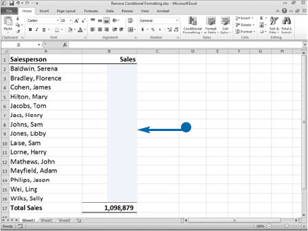
To delete the duplicates, select the cells from which you want to remove duplicates. Click the Data tab. Click Remove Duplicates in the Data Tools group. The Remove Duplicates dialog box appears. Click the check box to deselect the columns you do not want to check for duplicates (
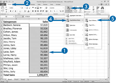
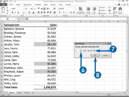
You can use conditional formatting to find the highest or lowest ranked values. For example, you can use conditional formatting to find the top three sales people or the bottom three sales people. When trying to find the rank, you have several options to choose from. If you choose Top 10, you can highlight the highest numbers in the selected range. You set the criteria: top 3, top 10, or whatever number you want. If you choose Bottom 10 items, you can choose the lowest number in the selected range, again you choose the criteria. If you want to find the top values or bottom values based in a percentage, choose Top 10 % or Bottom 10 % or enter the exact percentage you want.
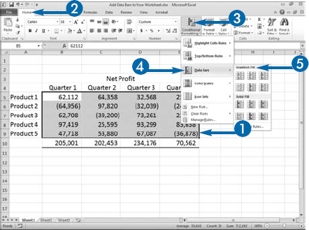
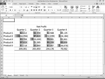
Data bars are a type of conditional formatting. You use data bars to indicate the relative size of a number — the longer the bar, the higher the number. Because each bar represents the relative size of the data, you can compare things such as sales performance with a glance.
Like all conditional formats, data bars can be applied to columns of data, rows of data, or a grid of data. When you add data bars to rows of data, make sure that the columns are the same size. Differences in the width of cells can distort the size of the bars. You can choose from several colors when you add data bars to your worksheet, and you can choose from solid color or gradient color.
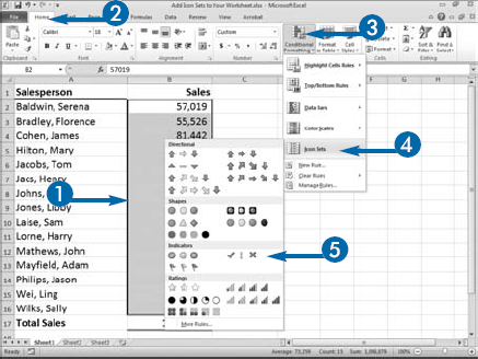
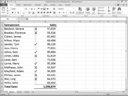
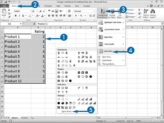
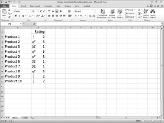
You can conditionally format your data by using icon sets. Icon sets make it easy to see trends in your data at a glance and they make it easy to see how data values relate to one another. Icon sets comes in sets of three, four, and five icons. You can use them to divide your data into three, four, or five categories. You choose the icon set you want to use. Excel automatically categorizes cells and places the correct icons in the cell. By default, Excel uses percentages to divide cells into categories.
Icons sets are a great way to group data. Each icon tells you a cell's value relative to all other values in the selected range.
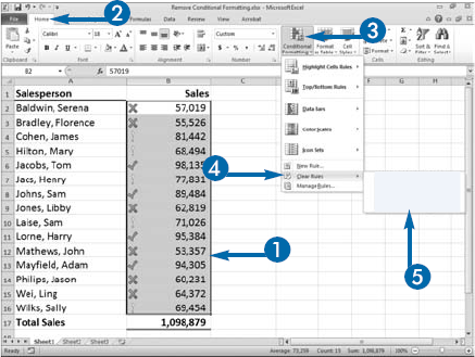
You can apply several types of conditional formats. Formats that highlight values that meet a criteria, data bars, color scales, and icon sets. When formats are no longer needed, you can remove them. When removing conditional formats you have four options: Remove Rules from Selected Cells, Clear Rules from Entire Sheet, Clear Rules from This Table, and Clear Rules from This PivotTable. Remove Rules from Selected Cells removes conditional formatting from the cells you have selected. Clear Rules from Entire Sheet removes all the conditional formatting on the worksheet. Clear Rules from This Table removes conditional formatting from the table you have selected. Clear Rules from This PivotTable removes conditional formatting from the PivotTable you have selected.
The Highlight Cells Rules and Top/Bottom Rules options under Conditional Formatting highlight cells that meet your criteria. You can, for example, use Highlight Cells Rules to find the top three sales people. A data bar is a colored bar you place in a cell. With data bars you can discern at a glance how large a value in one cell is relative to the values in other cells. The length of the bar represents the value of the cell relative to other cells — the longer the bar, the higher the value. Excel provides you with several bars from which to choose. Color scales and icon sets are similar to data bars, except color scales use gradations of color to represent the relative size of the value, and icon sets use icons to represent the relative size of the value.
Highlight cells rules, top/bottom rules, data bars, color scales, and icon sets all use rules to determine when to display what. You can use the rules defined by Excel or you can create your own. At the bottom of the Highlight Cells Rules, Top/Bottom Rules, Data Bars, Color Scales, or Icon Sets submenu, click More Rules to adjust and create rules. You can create rules that format cells based on their values, what they contain, how they rank, whether they are above or below average, and whether they are unique or duplicate values; or you can also use a formula to tell Excel which cells to format.
Change Conditional Formatting Rules
A menu appears.
A submenu appears.
The New Formatting Rule dialog box appears.
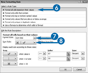
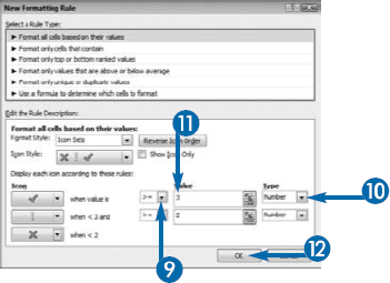
Note: You can choose Number, Percent, Formula, or Percentile.
Repeat Steps 9 through 11 for each icon, as needed.
Excel displays the results of your rule.
Extra
You can apply multiple conditional formatting rules to a range of cells. When you apply conditional formatting rules to cells, Excel executes them in order of precedence. By default, rules stack in the order you create them. Excel gives the most recently created rule the highest precedence. If two rules conflict, Excel applies the rule with the highest precedence. For example, if one rule formats text green and another rule formats text blue, Excel applies the rule with the highest precedence. You can click the Home tab, click Conditional Formatting, and then click Manage Rules to open the Conditional Formatting Rules Manager. The manager lists rules in order, putting the rule with the highest precedence on top. Use the Up and Down arrow keys (
If you manually apply a format to a cell and the format conflicts with a conditional format rule, the conditional format rule overrides the manual format. If you remove the conditional format, Excel reapplies the manual format.
By clicking the Copy button on the Home tab, pressing Ctrl+C, or clicking Copy on a context menu, you can easily copy the contents of a range of cells so you can paste the contents somewhere else in your worksheet. Cells can contain a lot of information. When you paste with Paste Special, you decide exactly what information you want to paste.
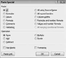
You can choose to paste everything or you can choose to paste just one element of the cell's contents, such as the formula, value, format, comment, validation, or column width. You can use the Paste Special dialog box to choose what you want to paste; however, you do not have to open the Paste Special dialog box to perform some paste special options, such as paste formulas, paste without borders, transpose, or paste-link. You can select these options and others directly from the Paste menu.
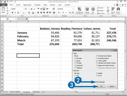
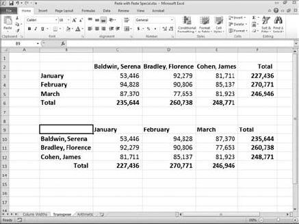
When you paste without borders, Excel pastes all your formatting but does not include any borders. When you transpose, Excel changes a row to a column or vice versa. You can use the paste link option in the Paste Special dialog box to keep your source and destination data synchronized. If you click the Paste Link button when pasting, Excel automatically updates the destination data when you make changes to the source data.
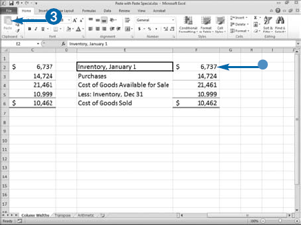
You can paste more than once. For example, when you paste by clicking Paste on the Home tab, Excel pastes the values, formulas, and formats but does not adjust the column widths. You can remedy this problem by pasting in two steps. In the first step, paste column widths. Excel adjusts the column widths. In the second step, paste your values, formulas, and formats.
Paste with Paste Special
Open the Paste Special Dialog Box
A menu appears.
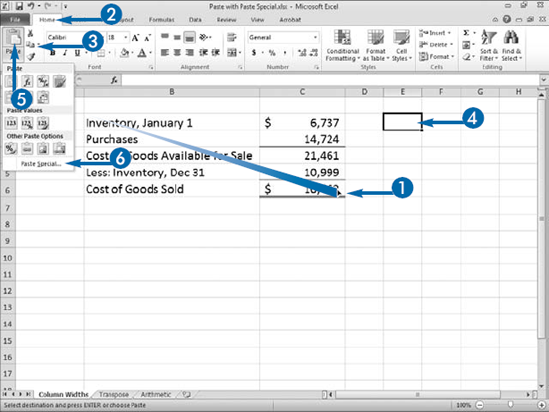
The Paste Special dialog box appears.
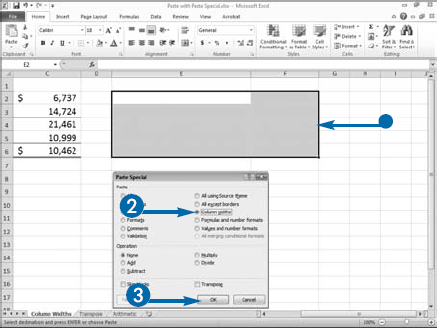
Excel copies the column widths from the source to the destination.
Excel pastes the contents of the cells.
You can press Esc to end the copy session.
You can use the Format Painter to copy formats from one cell to another. You can also use Paste Special. Simply copy a cell with the format you want, and then use Paste Special to paste the format into other cells. This feature is useful when you want to use the same format but different data in a range of cells. See Chapter 2 to learn more about the Format Painter.
You can use Paste Special to copy formulas or values from one location in your worksheet to another. When you want to use a cell's formula in adjacent cells in your worksheet, you can drag the fill handle to fill adjacent cells with the formula. However, when you want to use a formula in a nonadjacent cell, you must paste the formula with Paste Special. To learn more about using the fill handle, see the section "Extend a Series with AutoFill" in this chapter. When you want the results of a formula but not the formula, paste the value.
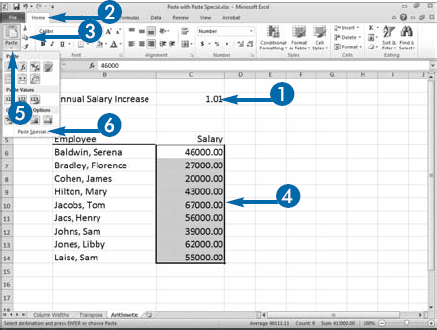
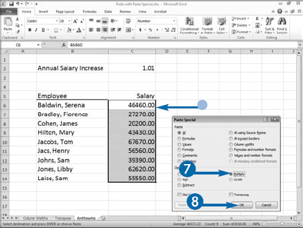
You can also use Paste Special to perform simple arithmetic operations on each cell in a range. For example, in a list of salaries, you may want to increase every salary by 1 percent. You can use Paste Special to make the change quickly. Just type 1.01 in a cell and then select Multiply in the Paste Special dialog box.
You can choose the Skip Blanks option in the Paste Special dialog box if your source data includes any blanks. If you choose this option, Excel will not overwrite a destination cell with a blank if the destination cell has data in it.