Excel's Function Wizard simplifies the use of functions. You can use the wizard with every one of Excel's functions, from the SUM function to complex statistical, mathematical, financial, or engineering functions.
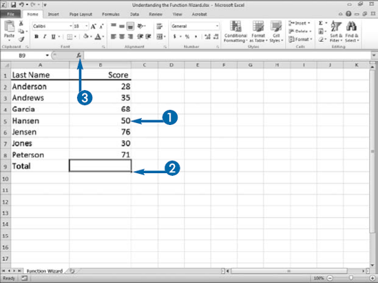
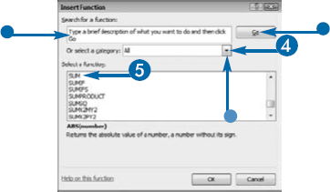
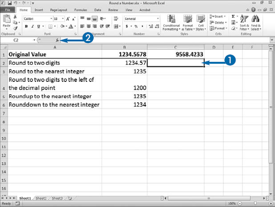
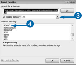
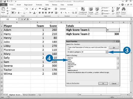
There are two ways to access the Function Wizard. You can select the cell where the result is to appear, click the Insert Function button (fx), and then use the Insert Function dialog box to find the function you want. The Insert Function dialog box provides you with two ways to find a function. You can type a description of the function in the Search for a Function field and then click Go. Excel will retrieve all the relevant functions and list them in the Select a Function field. Or, you can use the Or Select a Category field to select the category in which your function falls. Excel will list all the functions in that category in the Select a Function field. To open the Function Wizard, double click a function listed in Select a Function field.
Another way to access the Function Wizard is to select the cell where you want the results to appear. Type an equal (=) sign and the beginning of the function name. In the list of functions that appears, double-click the function you want and then click the Insert Function button. This method is quicker and is the best choice when you know the name of the function you want.
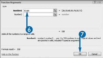
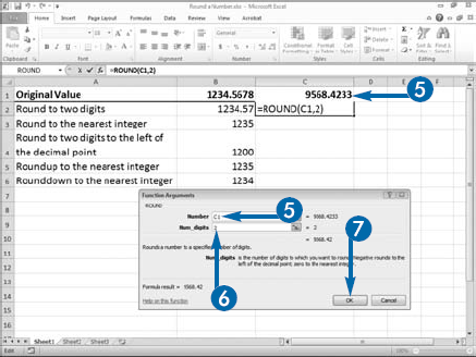
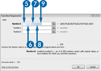
Both methods bring up the Function Arguments dialog box, where you can type the values you want to use in your calculation, type the range that contains the values, or click the cells containing the values you want.
Frequently, when you are creating a worksheet you will need to round numbers. Excel has several functions to aid you. The most commonly used is the ROUND function. This function rounds to the number of digits you specify. It takes two arguments: Number, the number you want to round, and Num_digits, the number of digits to which you want to round your number. If Num_digits is 1 or higher, Excel rounds to the number of decimal places you specify. If Num_digits is 0, Excel rounds to the nearest integer. If Num_digits is −1 or lower, Excel rounds to the number of digits you specify that are to the left of the decimal point. The function =ROUND(1234.5678,2) rounds to 1234.57, the function =ROUND(1234.5678,0) rounds to 1235, and the function =ROUND(1234.5678, −2) rounds to 1200.
When you use the ROUND function, if the digit you are rounding to is 5 or higher, Excel rounds up. If the digit is 4 or lower, Excel rounds down. If you only want Excel to round up, use the ROUNDUP function. If you only want Excel to round down, use the ROUNDDOWN function. Both ROUNDUP and ROUNDDOWN take the same two arguments as ROUND: Number and Num_digits.
Do not confuse rounding with number formatting. Rounding works by evaluating a number in an argument and rounding it to the number of digits you specify. When you format numbers, you simplify the appearance of numbers in the worksheet, making them easier to read. The underlying numbers do not change.
Round a Number


The Insert Function dialog box appears.


Alternatively, if the number is not in a cell, you can type the number into the Number field.

A negative number rounds to the left of the decimal point. A 0 rounds to the integer. A positive number rounds to the number of decimal places specified.

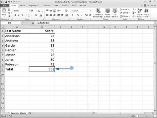
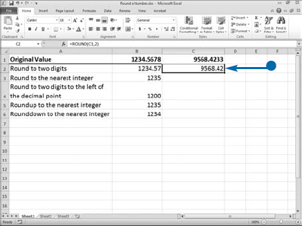
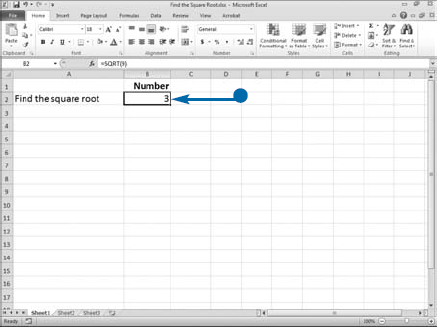
Excel rounds the number.
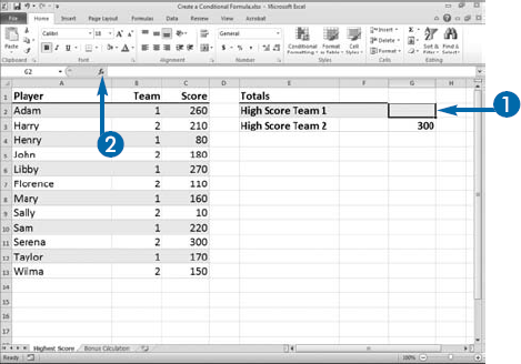
With a conditional formula, you can perform a calculation using values that meet a condition. For example, you can find the highest score for Team 1 from a list that consists of scores for Team 1 and Team 2.
A conditional formula often uses two functions. The first function, IF, defines the condition, or test, such as players on Team 1. To create the condition, you use a comparison operator, such as greater than (>), less than (<), greater than or equal to (>=), less than or equal to (<=), or equal to (=). If the condition evaluates to true, the second function is performed. The second function performs a calculation on numbers that meet the condition. Excel carries out the IF function first and then calculates the values that meet the condition defined in the IF function.
IF is an array function. It compares every number in a series to a condition and keeps track of the numbers that meet the condition. To create an array function, you press Ctrl+Shift+Enter instead of pressing the Enter key or clicking OK to complete your function. You must surround arrays with curly braces ({ }). Excel enters the curly braces automatically when you press Ctrl+Shift+Enter but not when you press Enter or click OK.
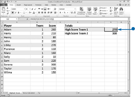
You can interpret the formula {=MAX(IF(B2:B13=1,C2:C13))} as follows: If the value in a cell between B2 and B13 is equal to 1, find the highest corresponding value in a cell between C2 and C13.
IF has an optional third argument. Use the third argument when you want to specify what happens when the condition is not met.
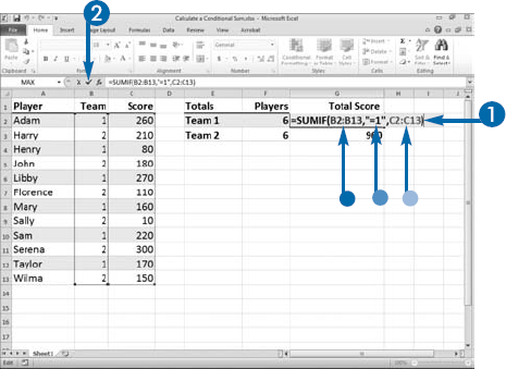
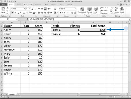
The SUMIF function combines the SUM and IF functions. SUMIF enables you to avoid complicated nesting and use the Function Wizard without making one function an argument of another.
SUMIF takes three arguments: Range, the range where you want to test a condition; Criteria, the condition you want to test; and Sum_range, the corresponding range you want to sum if the condition is met. For example, you can create a function that evaluates a list to determine if people are on Team 1, and if so, sum their scores. The third argument, the range to which the condition applies, is optional. If you exclude it, Excel sums the range you specify in the Range argument.
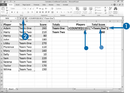
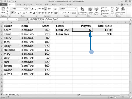
The COUNTIF function works like SUMIF. It combines two functions (COUNT and IF) and takes two arguments: Range, a series of values; and Criteria, the condition by which Excel tests the values. Whereas SUMIF sums the values, COUNTIF counts the number of items that passed the test. For example, you can create a function that evaluates a list to determine the team a person is on, and then counts all the people on Team One.
As with SUMIF, you can apply conditions to values and text. You can interpret the formula =COUNTIF(B2:B13,"=Team One") as count all the values in the cells between B2 and B13 that are equal to Team One.
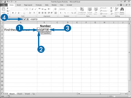
You can use the SQRT function to find the square root of a number. You can find the square root by entering the number you want the square root of into your worksheet or, if you do not want the number to appear in your worksheet, you can enter the number directly into the formula.
Excel can only calculate the square roots of positive numbers. If a negative number is the argument, as in SQRT(−9) Excel returns the error #NUM. If you want to calculate the positive square root of a negative number, find the absolute value of the number first by using the ABS function. The ABS function returns a number without its sign. The following formula returns 3, =SQRT(ABS(−9)).
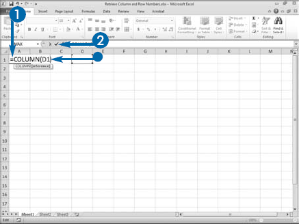
When you use functions such as VLOOKUP or INDEX you enter a column number, a row number, or both. See the sections, "Using VLOOKUP" and "Using INDEX," to learn more. If you enter an actual number, when you copy the function to another cell, the column or row number does not change. If you want the number to change in the same way relative cell addresses change, use the COLUMN function or the ROW function.
Both the COLUMN and ROW functions take one optional argument, Reference, the cell or cell range for which you want to retrieve the row or column number. If you enter one of these functions without a cell reference, =COLUMN() or =ROW(), Excel returns the column or row number of the current cell.
Retrieve Column or Row Numbers
The cell or cell range for which you want to obtain the column number.
Alternatively, enter the
ROWfunction.
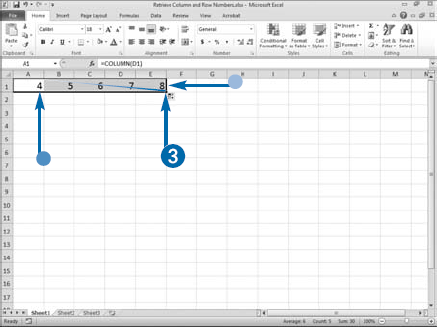
Excel displays the column number.
Note: See Chapter 12 to learn more about AutoFill.
Excel copies in a fashion similar to copying a relative cell address.
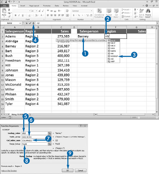
The VLOOKUP function searches the first column in your list, and when it finds the value that you are looking for, it returns another value in the same row. For example, you have a list, and in the first column there are names; in the second column there are regions; and in the third column there are sales numbers. If you have a name and you want to find the region, VLOOKUP can search for the name and return the region.
The first column of your list must contain the values you want to use to retrieve another value and you must sort the first column in ascending order. VLOOKUP has three required arguments: Lookup_value, the value or the cell address containing the value you want to use to retrieve another value; Table_array, the list's cell range; and Col_index_num, the column that contains the value you want to retrieve. The first column in the Table_array is column 1, the second column is column 2, and so on. If you use the COLUMN function to obtain the column number, when you copy your formula the cell reference will change. See section "Retrieve Column or Row Numbers" to learn more.
The VLOOKUP function has an optional fourth argument called Range_lookup. If you enter TRUE or leave the argument blank, the function looks for the closest match to the value you seek. If you enter FALSE, the function returns exact matches only.
If you are searching text data, make sure the column you are searching does not contain any nonprinting characters, leading spaces, or trailing spaces, and that curly or straight quotation marks are used consistently. If you are searching for numbers or dates, make sure they are not formatted as text. These situations can cause VLOOKUP to bring back an unexpected result.
Using VLOOKUP
As you begin to type, the Function AutoComplete list appears.
The Function Arguments dialog box appears.


The cell containing the formula displays the value corresponding to the lookup value.

Note: See Chapter 3 to learn how to copy and paste.
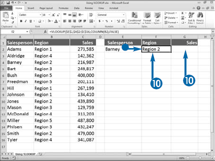

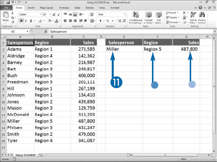
The cell containing the formula displays the value corresponding to the lookup value.
The cell you copied and pasted retrieves the next column.
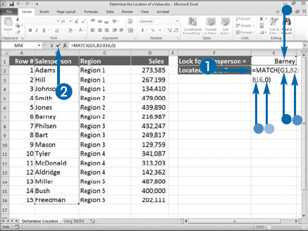
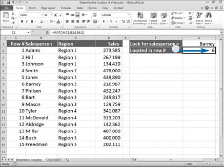
To determine the relative location of a value within a row or column, you can use the MATCH function. For example, if you have a list and you want to find which row in the list the salesperson named Barney is located, you can use the MATCH function.
The MATCH function needs three pieces of information: Lookup_value, Lookup_array, and Match_type. The Lookup_value is the value you want to find. The Lookup_array is the range you want to search. The Match_type is a number that tells Excel how to match values from the Lookup_value argument to the Lookup_array argument.
The Match_type is optional. If you omit it, or you enter a value of 1, Excel finds the largest value that is less than or equal to the Lookup_value. If you enter 0, Excel finds an exact match. If you enter −1, Excel returns the smallest value that is greater than or equal to the Lookup_value. If you omit the Match_type or enter a Match_type of 1, you must sort the Lookup_array in ascending order. If you enter a Match_type of 0, the Lookup_array can be in any order. If you enter a Match_type of −1, you must sort the Lookup_array in descending order. See Chapter 8 for more on sorting your data.
The MATCH function returns a number that identifies the relative location of the value within the specified range of cells. For example, if Excel returns the value 2 and the specified range of cells is B2 through B16, cell B3 contains the value, or the closest match. Excel interprets B2 to be the value 1, B3 to be value 2, B4 to be value 3, on so on.
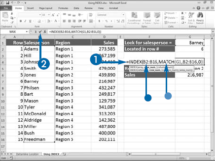
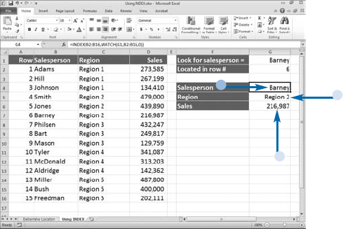
The MATCH function retrieves the relative position of a value. See the section, "Determine the Location of a Value" for a detailed explanation of the MATCH function. If you want to retrieve the actual value, use the INDEX function in conjunction with the MATCH function. The INDEX function has two forms. This example uses the Array form. The Array form takes three arguments: Array, the range from which you want to retrieve a value; Row_num, the position of the row you want to retrieve; and Col_num, the position of the column you want to retrieve. If the Array argument only contains one column, you do not need to specify the Col_num. If the Array argument only contains one row, you do not need to specify the Row_num.
In the following formula, =INDEX(B2:B16,MATCH(G1,B2:B16,0)), B2:B16 is the column that contains the value you want. The MATCH function retrieves the row you want. The formula could also be written =INDEX(B2:B16, 6). Cell B2 is row 1, B3 is row 2, and so on. The formula returns the value in cell B7, because it is on row 6.
When using the INDEX function, if you include both the Row_num and the Col_num arguments, Excel returns the value of the cell that is at the intersection of the row and column. For example, if you enter the formula =INDEX(B2:D16,6,3), Excel looks at the range B2 to D16 and returns the sixth row and third column.
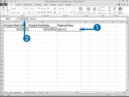
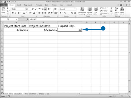
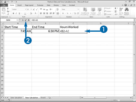
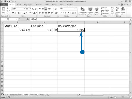
You can perform date and time calculations. You can find, for example, the number of days that have elapsed between the start of a project and the end of a project or the number of hours worked from the start of the workday to the end of the workday. Excel bases every date and time on a serial value that it can use to add and subtract.
Excel calculates a date's serial value as the number of days after January 1, 1900, and represents each date with a whole number. Excel calculates a time's serial value in units of 1/60th of a second. Each time can be represented as a serial value between 0 and 1. A date and time consists of the date to the left of the decimal and a time to the right. Take the example April 1, 2012 6:00 p.m. The date and time serial value is 41000.75. See Chapter 2 to learn more about dates and times.
Subtracting one date or time from another involves subtracting one serial value from another. For example, the serial value for April 1, 2012 is 41000. The serial value for May 21, 2012 is 41050. To obtain the number of days between April 1, 2012 and May 21, 2012 Excel performs the following calculation: = 41050 – 41000, which equals 50. Showing a date or time in the General format displays its serial value. When performing a date or time calculation, you do not need to display the serial value. Instead use date and time formats to display recognizable dates or times.
If you are calculating the number of hours that have elapsed, use the Format Cells dialog box and set the results of the calculation to the hour and minutes (13:30) time format.