A text box is a graphic that displays text. You draw the text box and then you type the text. You can add any amount of text to a text box; your text will automatically wrap when it reaches the width of the box. If you want your text box to be a perfect square, press and hold the Shift key as you click and drag to create the box. If you want it to align with the cell grid, press and hold the Alt key as you click and drag.
You can use a text box to create logos, add text to graphics, or annotate your worksheet. Additionally, you can apply a style, which is a set of formats, to a text box.

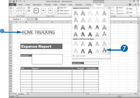
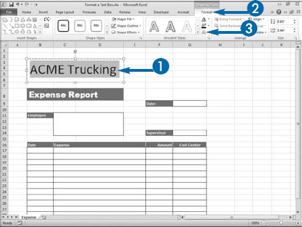
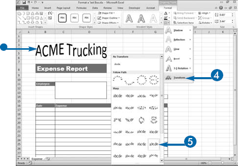
You can add text effects to a text box. You simply select the text and then apply the effect. You can create text with shadows, reflections, glows, bevels, 3-D rotations, and transforms. Shadows give the illusion that a light is being cast on the text. Reflections create a transparent mirror image. Glows create a transparent border around the text. Bevels give the text a 3-D look. 3-D rotations rotate the text so it appears three-dimensional. Transforms warp or place the text on a path. For each option, you can choose from several subgroups and you can apply multiple effects. You can combine text effects with styles and other formatting options.
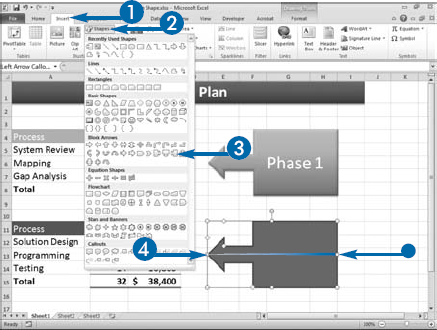
Shapes have a variety of purposes. For example, arrows point out relationships between data, and flowchart elements convey the structure of data. Excel provides a variety of shapes, including lines, rectangles, arrows, flowchart elements, stars, banners, and callouts — all of which you can use in your worksheet.
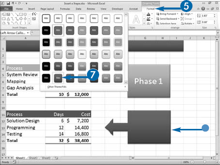
To create a shape you simply select a shape from the Shapes gallery and then click and drag to add the shape to your worksheet. Press and hold the Shift key while you click and drag if you want the shape to maintain its original proportions. Press and hold the Alt key as you click and drag if you want the shape to align with the table grid. A style is a predefined set of formats. You can apply a style to a shape.
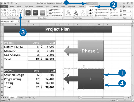
You can add text to a shape. You simply click the text button, click the shape, and then type the text. You can add any amount of text. Your text automatically wraps when it reaches the width of the box. When adding text, you can move to a new line at any time by pressing the Enter key.
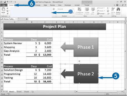
By default, Excel centers text and uses a default font, font color, and size. You can use most of the options on the Home tab in the Font and Alignment groups to format the text. For example, you can change the alignment, change the font, change the font size, and change the font color, apply bold, italics, underlines, and more. To learn more about formatting text, see Chapter 2.
Add Text to a Shape

The Drawing tools appear.


You can now add text to the shape.

Excel adds your text.

You can use most of these options to format your text.
Note: See Chapter 2 to learn more about formatting.
You click a graphic object to select it. When you select a graphic object, handles appear on its top, bottom, sides, and corners. Square handles appear on the top, bottom and sides. Round handles appear on the corners. You can use these handle to resize the graphic. Drag the top or bottom handles to resize the graphic object vertically. Drag the side handles to resize the graphic object horizontally. Drag a corner handle to change the overall size of the graphic.
To select more than one graphic object, press and hold the Ctrl key as you select each object. If you have more than one object selected, when you resize one object, Excel resizes all the other selected objects.
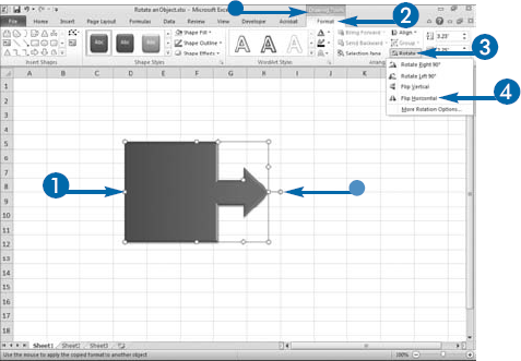
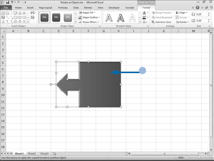
You can rotate any graphic object. For example, if you create a shape that points right and you want it to point left, you can rotate the shape so that it points left. When you select a graphic object, a rotation handle appears. To rotate the object, drag the rotation handle. If you want to constrain the rotation to intervals of 15 degrees, press and hold the Shift key as you drag.
You can use the Ribbon to rotate shapes 90 degrees left or 90 degrees right or to flip them vertically or horizontally. For example, if you have an arrow that is pointing to the right, you can select Flip Horizontal from the Rotate menu on the Format tab to flip it so it points left.
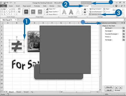
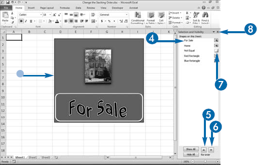
When you place a shape, text box, photograph, clip art, or any other type of graphic in your Excel worksheet, Excel stacks it. When graphics overlap, graphics that are higher in the stack appear to be on top of graphics that are lower in the stack. This can cause problems. For example, the text you want to place on a picture could actually appear behind the picture. Fortunately, you can change the stacking order. You can use the Selection and Visibility pane to choose the exact stack order to display your graphics.
Excel names each graphic as you create or add it to your worksheet. When you open the Selection and Visibility pane, these names display. You can change the Excel-generated names to names that are more meaningful.
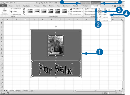
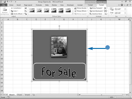
You can create a series of graphics that illustrate a single point. For example, you can create a set of graphics that show a house for sale. You may want to work with these graphics as a group. You can group graphics so that when you select one graphic, every graphic in the group is selected. You can move and resize grouped objects as if they were one object. You cannot edit, format, move, or size objects in a group individually until they are ungrouped. For example, if you apply an All Text in the Shape WordArt style to one object in the group, Excel applies it to all the objects in the group.
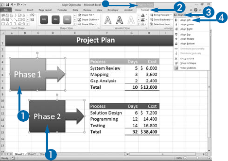
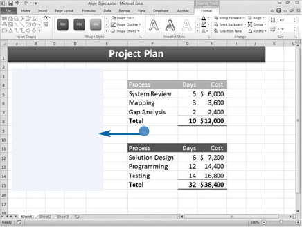
When you place graphic objects in a worksheet, you may want them to line up perfectly with one another. For example, you may want shapes you draw to be perfectly aligned. You can use Excel's alignment options to align objects left, center, right, top, middle, or bottom. When you align objects left, the left edges of all the objects are flush. When you align objects center, the vertical center of all the objects is uniform. When you align objects right, the right edges of all the objects are flush. When you align objects top, the top edges of all the objects are flush. When you align objects middle, the horizontal center of all the objects is uniform. And when you align objects bottom, the bottom edges of all the objects are flush.
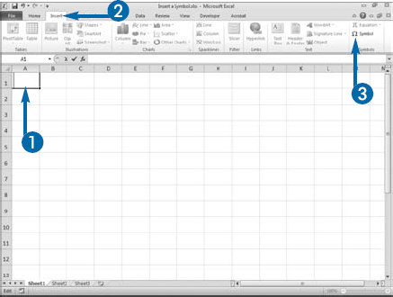
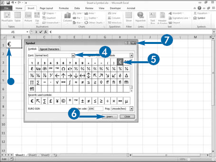
In Excel, you are not restricted to the standard numbers, letters, and punctuation marks on your keyboard. You can also select from hundreds of symbols, such as foreign letters, and currency characters, such as the Euro (€). Each font has a different set of symbols.
Symbols serve many uses in Excel. Many financial applications call for currency symbols. Symbols are useful in column and row heads as part of the text describing column or row content. For example, Net Sales in €.
Using a symbol in the same cell with a value such as a number, date, or time usually prevents the value from being used in a formula. If you need to use a special character in a cell that is referenced by a formula, use a number format.
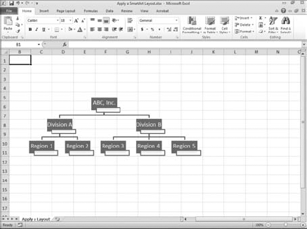
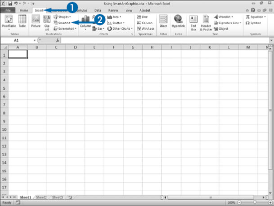
SmartArt graphics are predesigned layouts that you can use to illustrate your ideas. Presenting ideas as a graphic makes them easier to understand. For example, you can use a SmartArt graphic to create an organization chart. Excel provides the layout. All you have to do is enter the proper information.
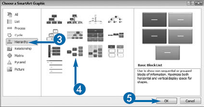
There are seven categories of SmartArt graphics: List, Process, Cycle, Hierarchy, Relationship, Matrix, and Pyramid. Each category has several layouts. Before you choose a graphic, consider carefully which category will best illustrate your ideas. Use the List category to show steps in a task, the sequence of events, or groups of related ideas; the Workflow category to show the progression of tasks or the sequence of events over time; the Cycle category to show the cycle of events or the stages of a project; the Hierarchy category to show hierarchical relationships; the Relationship category to show how ideas compare and contrast; the Matrix category to show how parts relate to the whole; and the Pyramid category to show the proportional relationship of parts to the whole.
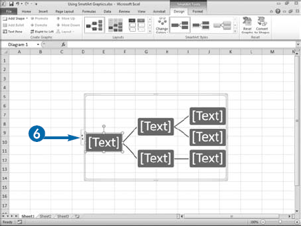
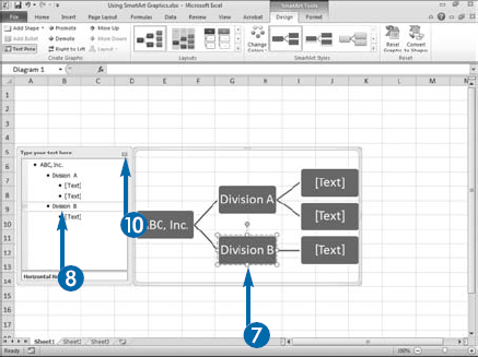
After you select a graphic, Excel places it in your worksheet. You can then type your information into the text box on the shapes or you can open the Text pane and type your information there. Excel adjusts the size of the font to fit the box. Your text will automatically wrap when it reaches the end of the box. If at any time you want to start a new line of text, press the Enter key.
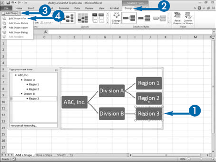
Each SmartArt graphic has a default number of shapes included. This number depends on the layout. You can use the Add Shape menu to add additional shapes to most layouts. For example, if you are creating an organization chart for your company and you have two regions at the third level, but the SmartArt layout you have chosen only has one shape at that level, you can add an additional shape.
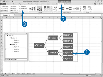
The Add Shape menu has four options: Add Shape After, Add Shape Before, Add Shape Above, and Add Shape Below. Add Shape After creates a new shape on the same level after the selected shape. Add Shape Before creates a new shape on the same level before the selected shape. Add Shape Above creates a new shape on the level above the selected shape. Add Shape Below creates a new shape on the level below the selected shape. You can use the Promote and Demote options in the Create Graphic group to move shapes up and down the levels. Promote moves a shape up a level. Demote moves a shape down a level. You can use Reorder Up and Reorder Down to move shapes up and down a stack. Reorder Up moves a shape up. Reorder Down moves a shape down.
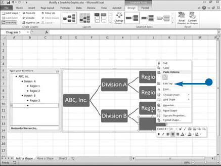
As you add shapes, Excel adjusts the size of the other shapes in the graphic, thereby keeping the size of all the shapes in proportion. When you add a new shape to a SmartArt graphic, you cannot immediately add text to it unless you use the Text pane, or right-click and then select Edit Text from the context menu.
Modify a SmartArt Graphic
Add a Shape
The SmartArt tools appear.
The Add Shape menu appears.
Excel adds a shape.
You can right-click and then select Edit Text from"the context menu to add text.
Move a Shape
SmartArt tools appear.
Alternatively, click Move Up to move up the stack; Promote, to move up a level; and Demote to move down a level.
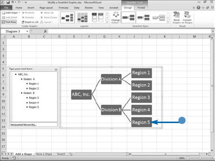
Excel moves the shape.
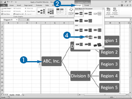
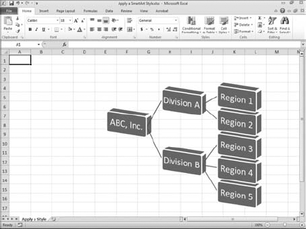
A style is a collection of formats. The formatting can consist of a fill, an outline, colors, fonts, and shape effects such as bevels, shadows, 3-D rotations, and much more. You could apply each of these formats individually to the objects in a SmartArt graphic, but by using a style, you can complete the process in just a few clicks.
One of the reasons you may want to change the style applied to a SmartArt graphic is to give your documents a consistent look and feel. You can, for example, apply the same style to all your graphics. Changing the style can dramatically change the look of a SmartArt graphic but it does not affect your SmartArt graphic content.
Excel divides SmartArt graphics into categories. Within each category there are several layouts from which you can choose. If after choosing a layout, you want to change to another layout, you can. Excel automatically transfers the data from your current layout to the new layout. For example, if you have created a horizontal organization chart but your manager prefers a vertical organization chart, you can make the change simply by changing the layout.
By default, the Layouts gallery displays layouts in the same category as your current layout. However, you can select a layout from another category. For example, if your current layout is from the Hierarchy category, you switch to the List category and then select a layout from there.