If you want to use the same data in multiple locations, you can copy and paste the data instead of retyping it. For example, you can copy a list of data in one worksheet to another worksheet, or you can copy a formula to multiple other cells. When you copy and perform a standard paste to a cell or range of cells, Excel duplicates everything in the original cell — including the cell values, formulas, formatting, comments, and data validation — and leaves the original cell unchanged.
If you want to move information from one location to another, you can cut the information, and then paste it. Cutting and pasting removes data from its current location and places it in a new location. For example, you can move a list of data in one worksheet to another worksheet, or you can move a formula to another cell.
After you cut or copy a range of cells, you can paste the cell contents to any location within your current workbook, another Excel workbook, or any other Microsoft Windows program. When you paste to an Excel workbook, Excel replaces the content of the cells you paste into with the cut or copied values. For that reason, be careful when you paste, because you can overwrite other data.
You can copy and paste or cut and paste multiple cells only if the cells are adjacent. When you apply the Cut or Copy command to a range of cells, Excel surrounds the cells with a dotted line. The selected cells remain marked until you paste the cells or press the Esc key to deselect them.
If you do not want to paste all of the cell's contents, use Paste Special, explained in Chapter 12, or use a live preview, explained in this chapter.
Copy, Cut, and Paste Cells
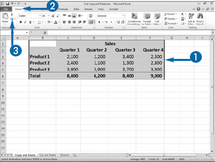
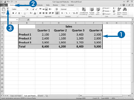
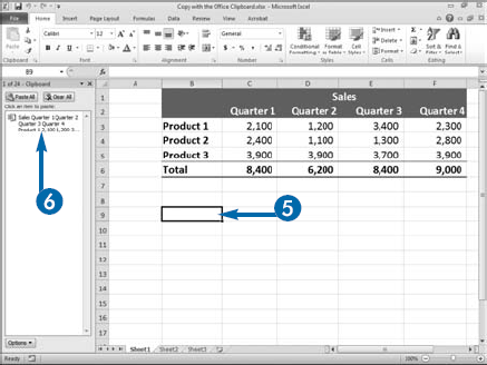
Copy And Paste


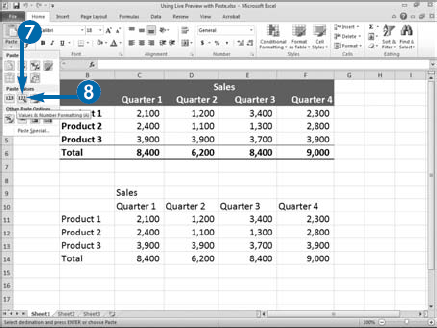
A dotted line appears around the cells you selected.


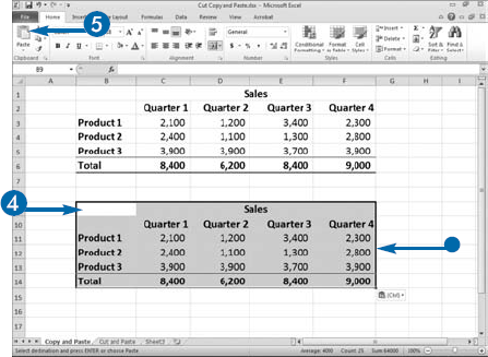
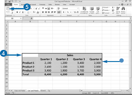
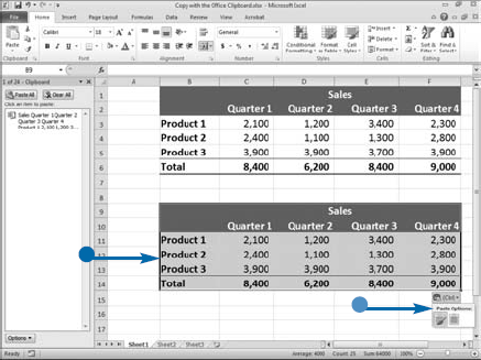
Excel places a copy of the copied cells in the new location.
A dotted line appears around the selected cells.
Excel places the data in the new location.
Apply It
To use your mouse to move a range of cells, select the cells you want to move and then point to the border of your selection. When your mouse pointer turns into a four-sided arrow (
You can select cells and then press Ctrl+C to copy or Ctrl+X to cut. You can then press Ctrl+V to paste.
When you cut or copy a range of cells that have hidden rows or columns and then paste them, Excel includes the hidden rows and/or columns. If you want to copy only visible cells, select the cells you want to copy. Click the Home tab. Click Find & Select in the Editing group. A menu appears. Click Go To Special. The Go To Special dialog box appears. Click Visible Cells Only. Click OK. Press Ctrl+C. Move to the paste area. Press Ctrl+V.
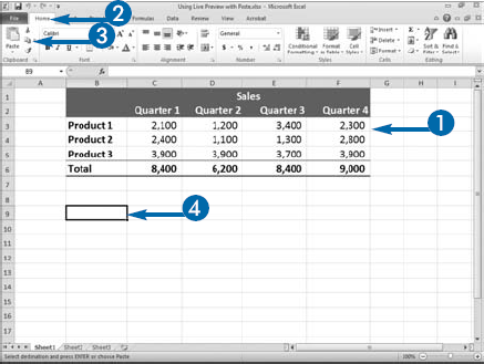
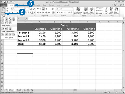
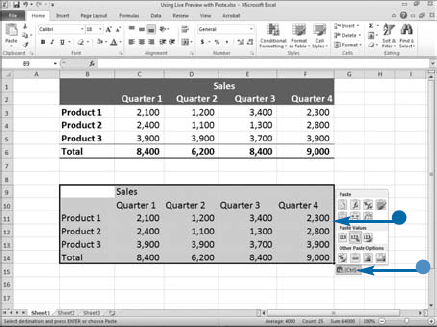
Starting with Office 2010, you can see a live preview of your paste by hovering over the choices in the Paste gallery. The Paste gallery provides you with a variety of paste options, such as Paste, Formulas, Values, and Formatting. If you choose Paste, Excel pastes everything. If you choose Formulas, Excel only pastes the formulas. If you choose Values, Excel does not paste the formulas, but instead pastes the results of the formulas. If you choose Formatting, Excel only pastes the formats.
You can view the Paste gallery by clicking the down arrow under the Paste button or by right-clicking and viewing the gallery on the context menu. The options that are available to you depend on what you have cut or copied and where you are pasting. For example, the choices you see when you are pasting from one area of an Excel worksheet to another area of an Excel worksheet are different from the choices you see when you are pasting from an Excel worksheet to a Word document.
As you hover over each option, Excel displays a tooltip and an accelerator key. The tooltip explains the option. You can click the option or press the accelerator key to apply the option. After you paste, an Options button appears. To change the type of paste, you can click the Options button and then select a different paste method. If you paste by pressing Ctrl+V, press the Ctrl key after pressing Ctrl+V to view the gallery of paste options and then select the option you want.
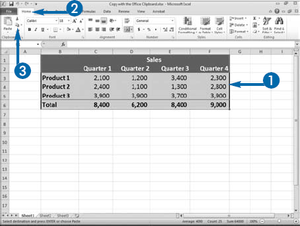
With Office, you can place data into a storage area called the Clipboard and then paste that data into Excel or another Office application. Cut and copied data stays on the Clipboard until you close all Office applications. The Office Clipboard can store up to 24 cut or copied items. When you add the 25th item, Office deletes the first item. You can store text and graphics on the Clipboard. As you add items to the Clipboard, they appear at the top of the Clipboard task pane. All the items on the Clipboard are available for you to paste to a new location in Excel or into another Office document.
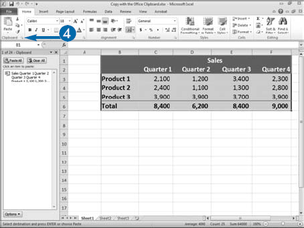
The Clipboard is not visible until you access it. In Excel, you access the Clipboard by clicking the launcher in the Clipboard group on the Home tab. Each item on the Clipboard appears with an icon that tells you the Office application the information originated from and shows a portion of the text or a thumbnail if the item is a graphic. You can use the Clipboard to store a range of cells. The Office Clipboard pastes the entire range, including all the values, but any formulas in the cells are not included when you paste.
You can paste everything on your Clipboard into your worksheet by clicking the Paste All button. You can clear the Clipboard by clicking the Clear All button.
After you paste an item from the Clipboard, Excel displays the Paste Options menu. You can use the menu to choose whether you want to use the source formatting or match the destination formatting.
As you develop your worksheets, you will sometimes want to make changes to the layout. For example, as you modify your worksheet, you may find that you need to insert or delete cells or even insert or delete entire columns or rows of cells. In Excel, you can shift a cell or group of cells up, down, left, or right. You can also add or delete columns and rows.
When you insert cells, columns, or rows, Excel automatically adjusts any formulas that reference the cells, whether they are relative or absolute. For example, if your formula reads =SUM(C2:C4) and you insert three rows anywhere between C2 and C4, your formula will automatically change to =SUM(C2:C7) to accommodate the three new rows. See Chapter 4 to learn more about relative and absolute cell references. When you delete cells, columns, and rows, Excel also automatically adjusts any formulas that reference the cells; however, if you delete a cell that you directly reference in a formula, Excel cannot adjust the formula and displays a #REF error instead.
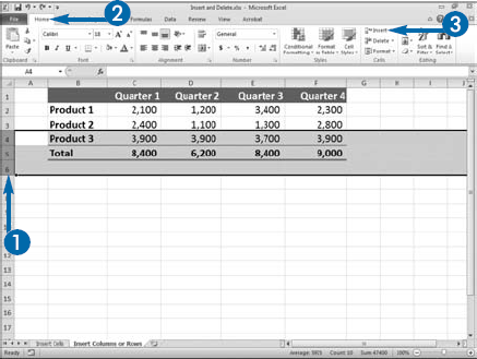
If you want to insert columns, select columns to the right of where you want the new columns and then click Insert. For example, if you want to insert three columns, select three columns and then click Insert. If you want to insert rows, select the number of rows below where you want the new rows and then click Insert. For example, if you want to insert three rows, select three rows and then click Insert. If you want to insert nonadjacent columns or rows, hold down the Ctrl key as you select where you want to place the columns or rows.
Insert or Delete
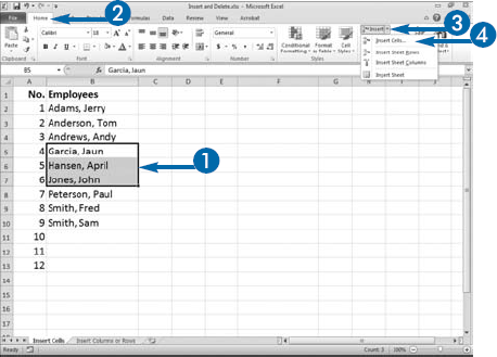
Insert Cells
A menu appears.
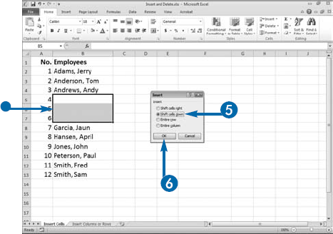
The Insert dialog box appears.

Excel shifts the cells.
Note: If you want to delete cells, select the cells, click Home, click the

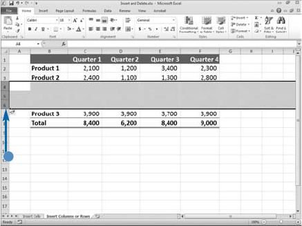
This example uses rows.
Excel inserts the columns or rows.
Excel adjusts the formulas.
Note: If you want to delete columns or rows, click and drag to select the column or row labels, click the Home tab, and then click Delete.
Extra
You can delete the contents of cells by selecting the cells and then pressing the Delete key. You can also use Excel's Clear options to remove everything or to delete formats, contents, or comments from a cell. To remove everything from a range of cells, select the cells, click the Home tab, click Clear (
To insert a new worksheet, press Shift+F11 or click the Insert Worksheet button (
As worksheets get larger, finding the information you want can be difficult. You can use Excel's Find feature to locate information. If you want to replace the found information with new information, use Excel's Find and Replace feature. Use the Find tab in the Find and Replace dialog box to find information. Use the Replace tab in the Find and Replace dialog box to find and replace information.
You can use substitutions in the Find and Replace dialog box. You can use the asterisk (*) as a substitute for any sequence of characters. You can use the question mark (?) as a substitute for any single character. For example, typing *ber finds September, October, November, and December. Typing J?ne finds Jane and June.
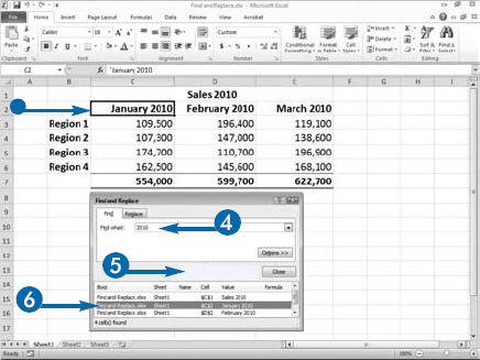
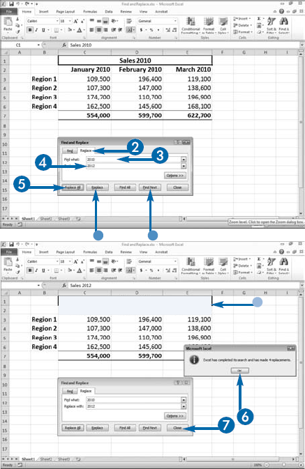
When you click the Find All button, by default Excel finds every instance of the value you are looking for in the active worksheet and lists the workbook, worksheet, cell name, cell address, value, and formula for each found value at the bottom of the Find and Replace dialog box. When you click Find Next, Excel moves to the first instance of the value. Excel moves to the next instance with every additional click of the Find Next button.
If you want to replace the values you find with a new value, click Replace All on the Replace tab to replace every instance of the value. Click Replace to replace the selected instance of the value and then move to the next instance. Click Find Next if you want to move to the next instance without replacing the selected instance.
In the Find and Replace dialog box, you can use the Options button to set additional options.
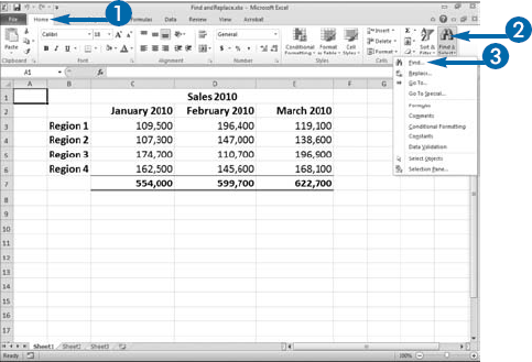
Find and Replace Information
Find Information
A menu appears.
The Find and Replace dialog box appears.
Excel moves to the instance you clicked.
Extra
You can click the Options button on the Find and Replace tabs in the Find and Replace dialog box to set several options. In the Within field, select Sheet if you want to search only the active worksheet or select Workbook if you want to search the entire workbook.
In the Search field, select By Rows if you want to search left to right across the rows. Select Column if you want to search top to bottom down the columns.
Select the check box in the Match Case field (
Select the check box in the Match Entire Cell Contents field (
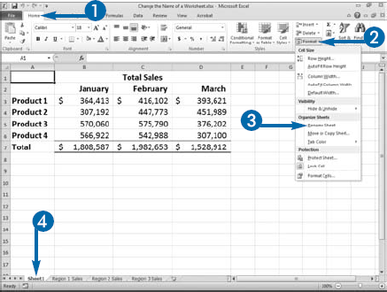
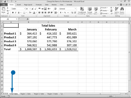
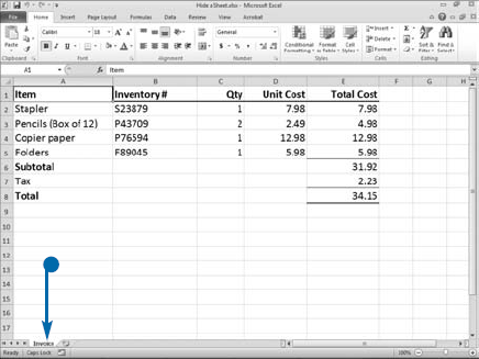
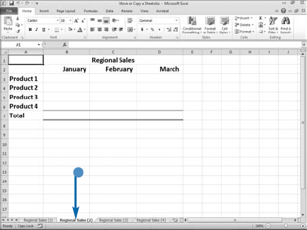
If you have a number of worksheets in your workbook, naming your sheets enables users to determine easily which sheet they want to access. For example, if you keep sales figures for three regions and you keep each region on a separate worksheet, you can name those worksheets Region 1 Sales, Region 2 Sales, and Region 3 Sales. If you keep total sales on yet another worksheet, you can name that worksheet Total Sales.
By default, Excel names all worksheets Sheet#, replacing # with a number that represents the order in which the sheet was added. For example, a typical workbook contains three sheets: Sheet1, Sheet2, and Sheet3. If you add a worksheet, Excel names it Sheet4. Excel uses the name Chart# for chart sheets.
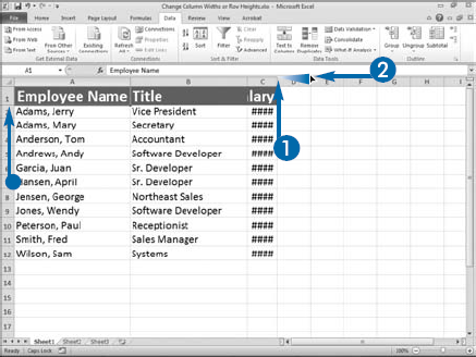
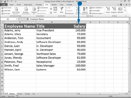
There are times when you may need to adjust a column width or row height. For example, text that is too long spills over into the next cell, numbers that are too long display as pound signs (####), and Excel cuts off fonts that are too large for the cell. To view the data, you can drag the right border of the column label to change the width of the cells or you can drag the bottom border of the row label to change the height of the cells.
Excel can automatically determine the proper height or width of a column or row. The AutoFit Row Height option automatically adjusts the height of rows. The AutoFit Column Width option automatically adjusts the width of columns.
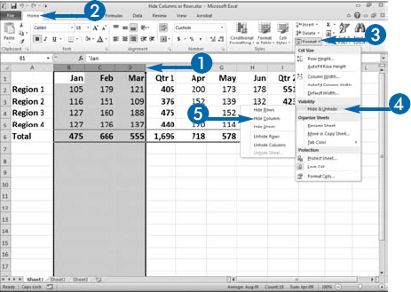
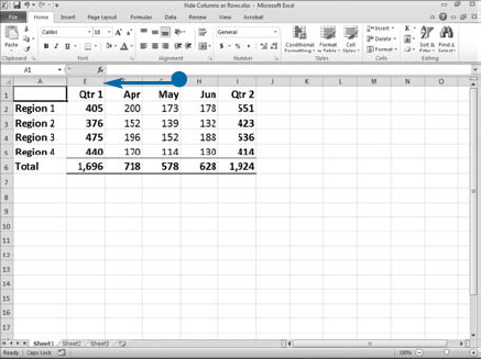
In Excel, you can hide columns or rows. You usually hide portions of a worksheet so that you can focus on the visible data. For example, a worksheet may contain monthly data and quarterly summaries. You can hide the monthly data so that you can focus on the quarterly summaries.
When you hide a column or row, you can still access the values contained in the cells when you reference them in formulas and functions. Excel indicates the existence of hidden columns and rows by skipping over the hidden columns and rows in the column and row labels. For example if you hide columns B, C, and D, you will only see column labels for A, E, F and so on.
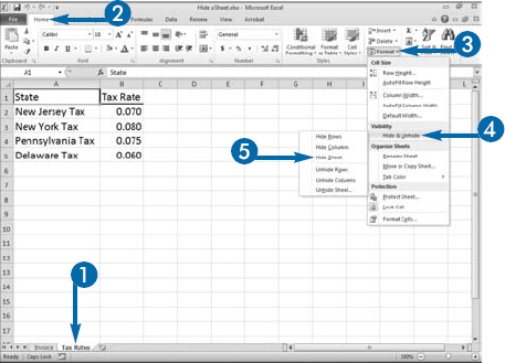
You can hide Excel worksheets. You may want to hide a worksheet to prevent users from viewing it. The worksheet might contain raw data that you use in calculations or to validate data entry. For example, in Chapter 4 you learn how to define constants. You may want to keep your constants in a hidden worksheet. In Chapter 13, you learn how to validate with a list. You may want to keep your validation lists in a hidden worksheet.
Hiding a worksheet does not always keep users from accessing it. Users can unhide sheets in Excel by using the Unhide option. If you want to prevent users from making changes to a hidden sheet, you must protect it. See Chapter 13 to learn how to protect a worksheet.
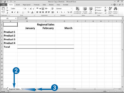
You can copy a worksheet. You can place a copy of a worksheet in the same workbook or you can place a copy of a worksheet in another workbook. For example, if you collect sales data for three regions on three separate worksheets and you format each worksheet the same, you can format one worksheet and then make copies of the worksheet so that you can use the copies when working on the other two regions.
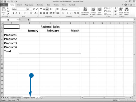
You can copy the worksheets to the same workbook or you can copy them to two separate additional workbooks — one for each region. When you copy a worksheet to the same workbook or if the workbook you are copying to already has a worksheet with the same name, Excel gives the worksheet the same name as the original worksheet and appends it with the copy number in parentheses.
You can rename the worksheet if you want. Before you can copy a worksheet to an existing workbook, the workbook must be open.
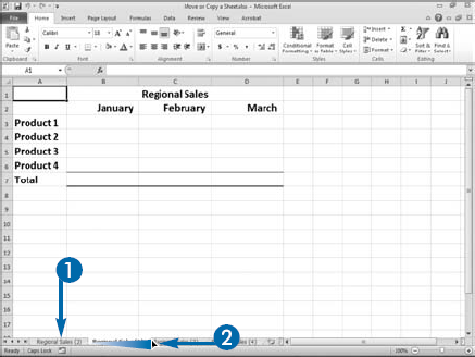
You can move a worksheet. For example, within a workbook, you can rearrange worksheets so that they appear alphabetically or in any other order you choose. You can also move a worksheet to another workbook. For example, if you keep sales data for three regions in a single workbook on three separate worksheets, you can move each worksheet to its own workbook. Be careful when you move a worksheet. If you have a formula that references the worksheet or if you have a chart that is based on the worksheet, moving the worksheet can cause errors.
Apply It
To copy a worksheet to an existing workbook, open the workbook. Right-click the worksheet's tab. A menu appears. Click Move or Copy Sheet. The Move or Copy dialog box appears. Click the down arrow (
To move a worksheet to an existing workbook, open the workbook. Right-click the worksheet's tab. A menu appears. Click Move or Copy Sheet. The Move or Copy dialog box appears. Click the down arrow in the To Book field and then select the workbook to which you want to move the worksheet. The sheets in the selected workbook appear in the Before Sheet box. Click the sheet you want to place the copied sheet before or click Move to End to make the sheet the last sheet in the workbook. Click OK. Excel moves the worksheet.
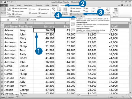
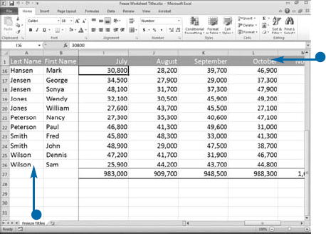
When you create a worksheet, you can create labels that identify the data in the columns and rows. For example, if you are collecting sales figures by sales person by month, you can place the month at the top of each column and the sales person's first and last name in the first two columns of each row. If you have more columns or rows than will fit on a screen, as you scroll down or across the window, the column and row labels you created disappear from view. You can freeze the column and row labels so that they remain in view as you scroll. You can freeze both the column and row labels. Or, you can freeze just column labels or just row labels.
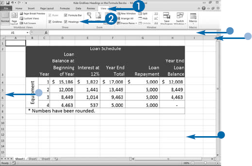
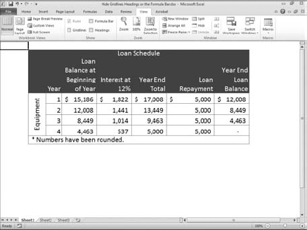
Gridlines are the faint lines that appear by default and separate the rows and columns in an Excel worksheet. Borders are a type of formatting that you can apply to cells to separate the rows and columns in a worksheet. To make borders stand out, you can hide gridlines.
Headings are the row and column labels that appear along the side and across the top of an Excel worksheet. If they are not relevant to the task you are preforming or if you want to make more room on your screen, you can remove them from view.
The formula bar appears below the Ribbon and displays the value or formula in the active cell. If you want to suppress the display of formulas, you can hide the formula bar.