19

Using Ranges

The Range object is probably the object you will utilize the most in your VBA code. A Range object can be a single cell, a rectangular block of cells, or the union of many rectangular blocks (a non-contiguous range). A Range object is contained within a Worksheet object.

The Excel object model does not support three-dimensional Range objects that span multiple worksheets – every cell in a single Range object must be on the same worksheet. If you want to process 3D ranges, you must process a Range object in each worksheet separately.

In this chapter, we will examine the most useful properties and methods of the Range object.

Activate and Select

The Activate and Select methods cause some confusion, and it is sometimes claimed that there is no difference between them. To understand the difference between them, we need to first understand the difference between the ActiveCell and Selection properties of the Application object. The screen in Figure 19-1 illustrates this.

Selection refers to B3:E10. ActiveCell refers to C5, the cell where data will be inserted if the user types something. ActiveCell only ever refers to a single cell, while Selection can refer to a single cell or a range of cells. The active cell is usually the top left-hand cell in the selection, but can be any cell in the selection, as shown in Figure 19-1. You can manually change the position of the active cell in a selection by pressing Tab, Enter, Shift+Tab, or Shift+Enter.

You can achieve the combination of selection and active cell shown previously by using the following code:

Public Sub SelectAndActivate()
  Range(“B3:E10”).Select
  Range(“C5”).Activate
End Sub

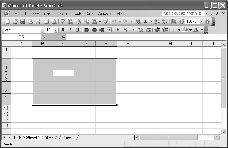
Figure 19-1

If you try to activate a cell that is outside the selection, you will change the selection, and the selection will become the activated cell.

Confusion also arises because you are permitted to specify more than one cell when you use the Activate method. Excel's behavior is determined by the location of the top-left cell in the range you activate. If the top-left cell is within the current selection, the selection does not change and the top-left cell becomes active. The following example will create the previous screen:

Public Sub SelectAndActivate2()
  Range(“B3:E10”).Select
  Range(“C5:Z100”).Activate
End Sub

If the top-left cell of the range you activate is not in the current selection, the range that you activate replaces the current selection as shown by the following:

Public Sub SelectAdActivate3()
  Range(“B3:E10”).Select
  Range(“A2:C52).Activate
End Sub

In this case, the Select is overruled by the Activate and A2:C5 becomes the selection.

Range Property

You can use the Range property of the Application object to refer to a Range object on the active worksheet. The following example refers to a Range object that is the B2 cell on the currently active worksheet:

Application.Range(“B2”)

Note that you can't test code examples like the previous one as they are presented. However, as long as you are referring to a range on the active worksheet, these examples can be tested by the immediate window of the VBE, as follows:

Application.Range(“B22).Select

It is important to note that the previous reference to a Range object will cause an error if there is no worksheet currently active. For example, it will cause an error if you have a chart sheet active.

As the Range property of the Application object is a member of <globals>, you can omit the reference to the Application object, as follows:

Range(“B2”)

You can refer to more complex Range objects than a single cell. The following example refers to a single block of cells on the active worksheet:

Range(“A1:D10”)

And this code refers to a non-contiguous range of cells:

Range(“A1:A10, C1:C10,E1:E10”)

The Range property also accepts two arguments that refer to diagonally opposite corners of a range. This gives you an alternative way to refer to the A1:D10 range:

Range(“A1”,“D10”)

Range also accepts names that have been applied to ranges. If you have defined a range of cells with the name SalesData, you can use the name as an argument:

Range(“SalesData”)

The arguments can be objects as well as strings, which provides much more flexibility. For example, you might want to refer to every cell in column A from cell A1 down to a cell that has been assigned the name LastCell:

Range(“A1”, Range(“LastCell”))

Shortcut Range References

You can also refer to a range by enclosing an A1 style range reference or a name in square brackets, which is a shortcut form of the Evaluate method of the Application object. It is equivalent to using a single string argument with the Range property, but is shorter:

[B2]
[A1:D10]
[A1:A10, C1:C10, E1:E10]
[SalesData]

This shortcut is convenient when you want to refer to an absolute range. However, it is not as flexible as the Range property as it cannot handle variable input as strings or object references.

Ranges on Inactive Worksheets

If you want to work efficiently with more than one worksheet at the same time, it is important to be able to refer to ranges on worksheets without having to activate those worksheets. Switching between worksheets is slow, and code that does this is more complex than it need be. Switching between worksheets in code is unnecessary and makes your solutions harder to read and debug.

All our examples so far apply to the active worksheet, because they have not been qualified by any specific worksheet reference. If you want to refer to a range on a worksheet that is not active, simply use the Range property of the required Worksheet object:

Worksheets(“Sheet1”).Range(“C10”)

If the workbook containing the worksheet and range is not active, you need to further qualify the reference to the Range object as follows:

Workbooks(“Sales.xls”).Worksheets(“Sheet1”).Range(“C10”)

However, you need to be careful if you want to use the Range property as an argument to another Range property. Say, you want to sum A1:A10 on Sheet1, while Sheet2 is the active sheet. You might be tempted to use the following code, which results in a runtime error:

MsgBox WorksheetFunction.Sum(Sheets(“Sheet1”).Range(Range(“A1”), _ Range(“A10”)))

The problem is that Range(“A1”) and Range(“A10”) refer to the active sheet, Sheet2. You need to use fully qualified properties:

MsgBox WorksheetFunction.Sum(Sheets(“Sheet1”).Range( _
                             Sheets(“Sheet1”).Range(“A1”), _
                 Sheets(“Sheet1”).Range(“A10”)))

When you need to refer to multiple instances of the same value you can abbreviate your code with a With..End With construct as follows:

With Sheets(“Sheet1”)
   MsgBox WorksheetFunction.Sum(.Range(.Range(“A1”), .Range(“A10”)))
End With

Range Property of a Range Object

The Range property is normally used as a property of the Worksheet object. You can also use the Range property of the Range object. In this case, it acts as a reference relative to the Range object itself. The following is a reference to the D4 cell:

Range(“C3”).Range(“B2”)

If you consider a virtual worksheet that has C3 as the top-left cell, and B2 is one column across and one row down on the virtual worksheet, you arrive at D4 on the real worksheet.

You will see this “Range in a Range” technique used in code generated by the macro recorder when relative recording is used (discussed in Chapter 1). For example, the following code was recorded when the active cell and the four cells to its right were selected while recording relatively:

ActiveCell.Range(“A1:E1”).Select

As the preceding code can be confusing, it is best to avoid relative cell referencing. The Cells property is a much better way to reference cells relatively.

Cells Property

You can use the Cells property of the Application, Worksheet, or Range objects to refer to the Range object containing all the cells in a Worksheet object or Range object. The following two lines of code each refer to a Range object that contains all the cells in the active worksheet:

ActiveSheet.Cells
Application.Cells

As the Cells property of the Application object is a member of <globals>, you can also refer to the Range object containing all the cells on the active worksheet as follows:

Cells

You can use the Cells property of a Range object as follows:

Range(“A1:D10”).Cells

However, the Cells property in the preceding statement simply refers to the original Range object it qualifies.

You can refer to a specific cell relative to the Range object by using the Item property of the Range object and specifying the relative row and column positions. The row parameter is always numeric. The column parameter can be numeric or you can use the column letters entered as a string. The following are both references to the Range object containing the B2 cell in the active worksheet:

Cells.Item(2,2)
Cells.Item(2,“B”)

As the Item property is the default property of the Range object, you can omit it as follows:

Cells(2,2)
Cells(2,“B”)

The numeric parameters are particularly useful when you want to loop through a series of rows or columns using an incrementing index number. The following example loops through rows 1 to 10 and columns A to E in the active worksheet, placing values in each cell:

Public Sub FillCells()
  Dim i As Integer, j As Integer

  For i = 1 To 10
    For j = 1 To 5
     Cells(i, j).Value = i * j
    Next j
  Next i
End Sub

Figure 19-2 shows the results of this code.

Cells used in Range

You can use the Cells property to specify the parameters within the Range property to define a Range object. The following code refers to A1:E10 in the active worksheet:

Range(Cells(1,1), Cells(10,5))

This type of referencing is particularly powerful because you can specify the parameters using numeric variables as shown in the previous looping example.

Ranges of Inactive Worksheets

As with the Range property, you can apply the Cells property to a worksheet that is not currently active:

Worksheets(“Sheet1”).Cells(2,3)

Figure 19-2

If you want to refer to a block of cells on an inactive worksheet using the Cells property, the same precautions apply as with the Range property. You must make sure you qualify the Cells property fully. If Sheet2 is active, and you want to refer to the range A1:E10 on Sheet1, the following code will fail because Cells(1,1) and Cells(10,5) are properties of the active worksheet:

Sheets(“Sheet1”).Range(Cells(1,1), Cells(10,5)).Font.Bold = True

A With…End With construct is an efficient way to incorporate the correct sheet reference:

With Sheets(“Sheet1”)
   .Range(.Cells(1, 1), .Cells(10, 5)).Font.Bold = True
End With

More on the Cells Property of the Range Object

The Cells property of a Range object provides a nice way to refer to cells relative to a starting cell, or within a block of cells. The following refers to cell F11:

Range(“D10:G20”).Cells(2,3)

If you want to examine a range with the name SalesData and color any figure under 100 red, you can use the following code:

Public Sub ColorCells()
  Dim Sales As Range
  Dim I As Long
  Dim J As Long

  Set Sales = Range(“SalesData”)
  For I = 1 To Sales.Rows.Count
    For J = 1 To Sales.Columns.Count
      If Sales.Cells(I, J).Value < 100 Then
        Sales.Cells(I, J).Font.ColorIndex = 3
      Else
        Sales.Cells(I, J).Font.ColorIndex = 1
      End If
    Next J
  Next I
End Sub

Figure 19-3 shows the result:

Figure 19-3

It is not, in fact, necessary to confine the referenced cells to the contents of the Range object. You can reference cells outside the original range. This means that you really only need to use the top-left cell of the Range object as a starting point. This code refers to F11, as in the earlier example:

Range(“D10”).Cells(2,3)

You can also use a shortcut version of this form of reference. The following is also a reference to cell F11:

Range(“D10”)(2,3)

Technically, this works because it is an allowable shortcut for the Item property of the Range object, rather than the Cells property, as described previously:

Range(“D10”).Item(2,3)

It is even possible to use zero or negative subscripts, as long as you don't attempt to reference outside the worksheet boundaries. This can lead to some odd results. The following code refers to cell C9:

Range(“D10”)(0,0)

The following refers to B8:

Range(“D10”)(−1,−1)

The previous Font.Colorlndex example using Sales can be written as follows, using this technique:

Public Sub ColorCells()
  Dim Sales As Range
  Dim i As Long
  Dim j As Long

  Set Sales = Range(“SalesData”)
  For i = 1 To Sales.Rows.Count
    For j = 1 To Sales.Columns.Count
      If Sales(i, j).Value < 100 Then
        Sales(i, j).Font.ColorIndex = 4
      Else
        Sales(i, j).Font.ColorIndex = 1
      End If
    Next j
  Next i
End Sub

There is actually a small increase in speed, if you adopt this shortcut. Running the second example, the increase is about 5% on my PC when compared to the first example.

Single-Parameter Range Reference

The shortcut range reference accepts a single parameter as well as two. If you are using this technique with a range with more than one row, and the index exceeds the number of columns in the range, the reference wraps within the columns of the range, down to the appropriate row.

The following refers to cell E10:

Range(“D10:E11”)(2)

The following refers to cell D11:

Range(“D10:E11”)(3)

The index can exceed the number of cells in the Range object and the reference will continue to wrap within the Range object's columns. The following refers to cell D12:

Range(1D10:E11”)(5)

Qualifying a Range object with a single parameter is useful when you want to step through all the cells in a range without having to separately track rows and columns. The ColorCells example can be further rewritten as follows, using this technique:

Public Sub ColorCells()
  Dim Sales As Range
  Dim i As Long

  Set Sales = Range(“SalesData”)
    For i = 1 To Sales.Cells.Count
      If Sales(i).Value < 100 Then
        Sales(i).Font.ColorIndex = 5
      Else
        Sales(i).Font.ColorIndex = 1
      End If
  Next i
End Sub

In the fourth and final variation on the ColorCells theme, you can step through all the cells in a range using a For Each…Next loop, if you do not need the index value of the For…Next loop for other purposes:

Public Sub ColorCells()
  Dim aRange As Range

  For Each aRange In Range(“SalesData”)
    If aRange.Value < 100 Then
      aRange.Font.ColorIndex = 6
    Else
      aRange.Font.ColorIndex = 1
    End If
  Next aRange
End Sub

Offset Property

The Offset property of the Range object returns a similar object to the Cells property, but is different in two ways. The first difference is that the Offset parameters are zero based, rather than one based, as the term “offset” implies. These examples both refer to the A10 cell:

Range(“A10”).Cells(1,1)
Range(“A10”).Offset(0,0)

The second difference is that the Range object generated by Cells consists of one cell. The Range object referred to by the Offset property of a range has the same number of rows and columns as the original range. The following refers to B2:C3:

Range(“A1:B2”5).Offset(1,1)

Offset is useful when you want to refer to ranges of equal sizes with a changing base point. For example, you might have sales figures for January to December in B1:B12 and want to generate a three-month moving average from March to December in C3:C12. The code to achieve this is:

Public Sub MoveAverage()
  Dim aRange As Range
  Dim i As Long

  Set aRange = Range(“B1:B3”)
  For i = 3 To 12
    Cells(i, “C”).Value = WorksheetFunction.Round _
      (WorksheetFunction.Sum(aRange) / 3, 0)
    Set aRange = aRange.Offset(1, 0)
  Next i
End Sub

Figure 19-4 shows the result of running the code:

Figure 19-4

Resize Property

You can use the Resize property of the Range object to refer to a range with the same top left-hand corner as the original range, but with a different number of rows and columns. The following refers to D10:E10:

Range(“D10:F20”).Resize(1,2)

Resize is useful when you want to extend or reduce a range by a row or column. For example, if you have a data list, which has been given the name Database, and you have just added another row at the bottom, you need to redefine the name to include the extra row. The following code extends the name by the extra row:

With Range(“Database”)
  .Resize(.Rows.Count + 1).Name = “Database”
End With

When you omit the second parameter, the number of columns remains unchanged. Similarly, you can omit the first parameter to leave the number of rows unchanged. The following refers to A1:C10:

Range(“A1:B10”).Resize(, 3)

You can use the following code to search for a value in a list and, having found it, copy it and the two columns to the right to a new location. The code to do this is:

Public Sub FindIt()
  Dim aRange As Range

  Set aRange = Range(“A1:A12”).Find(What:=“Jun”, _
    LookAt:=xlWhole, LookIn:=xlValues)

  If aRange Is Nothing Then
    MsgBox “Data not found”
    Exit Sub
  Else
    aRange.Resize(1, 3).Copy Destination:=Range(“G1”)
  End If
End Sub

Figure 19-5 shows the result.

The Find method does not act like the Edit Find command. It returns a reference to the found cell as a Range object but it does not select the found cell. If Find does not locate a match, it returns a null object that you can test for with the Is Nothing expression. If you attempt to copy the null object, a runtime error occurs.

SpecialCells Method

When you press the F5 key in a worksheet, the Go To dialog box appears. You can then press the Special… button to show the dialog box in Figure 19-6.

Figure 19-5

Figure 19-6

This dialog box allows you to do a number of useful things, such as find the last cell in the worksheet or all the cells with numbers rather than calculations. As you might expect, all these operations can be carried out in VBA code. Some have their own methods, but most of them can be performed using the SpecialCells method of the Range object.

Last Cell

The following code determines the last row and column in the worksheet:

Public Sub SelectLastCell()
  Dim aRange As Range
  Dim lastRow As Integer
  Dim lastColumn As Integer

  Set aRange = Range(“A1”).SpecialCells(xlCellTypeLastCell)
  lastRow = aRange.Row
  lastColumn = aRange.Column

  MsgBox lastColumn
End Sub

The last cell is considered to be the intersection of the highest numbered row in the worksheet that contains information and the highest numbered column in the worksheet that contains information. Excel also includes cells that have contained information during the current session, even if you have deleted that information. The last cell is not reset until you save the worksheet.

Excel considers formatted cells and unlocked cells to contain information. As a result, you will often find the last cell well beyond the region containing data, especially if the workbook has been imported from another spreadsheet application, such as Lotus 1-2-3. If you want to consider only cells that contain data in the form of numbers, text, and formulas, you can use the following code:

Public Sub GetRealLastCell()
  Dim realLastRow As Long
  Dim realLastColumn As Long
  Range(“A1”).Select

  On Error Resume Next
  realLastRow = Cells.Find(“*”, Range(“A1”), _
    xlFormulas, , xlByRows, xlPrevious).Row
  realLastColumn = Cells.Find(“*”, Range(“A1”), _
    xlFormulas, , xlByColumns, xlPrevious).Column
  Cells(realLastRow, realLastColumn).Select
End Sub

In this example, the Find method searches backwards from the A1 cell (which means that Excel wraps around the worksheet and starts searching from the last cell towards the A1 cell) to find the last row and column containing any characters. The On Error Resume Next statement is used to prevent a runtime error when the spreadsheet is empty.

If you want to get rid of the extra rows containing formats, you should select the entire rows, by selecting their row numbers, and then use Edit Delete to remove them. You can also select the unnecessary columns by their column letters, and delete them. At this point, the last cell will not be reset. You can save the worksheet to reset the last cell, or execute ActiveSheet.UsedRange in your code to perform a reset. The following code will remove extraneous rows and columns and reset the last cell:

Public Sub DeleteUnusedFormats()
  Dim lastRow As Long
  Dim lastColumn As Long
  Dim realLastRow As Long
  Dim realLastColumn As Long

  With Range(“A1”).SpecialCells(xlCellTypeLastCell)
    lastRow = .Row
    lastColumn = .Column
  End With

  realLastRow = Cells.Find(“*”, Range(“A1”), _
    xlFormulas, , xlByRows, xlPrevious).Row

  realLastColumn = Cells.Find(“*”, Range(“A1”), _
    xlFormulas, , xlByColumns, xlPrevious).Column

  If realLastRow < lastRow Then
    Range(Cells(realLastRow +1, 1), _
      Cells(lastRow, 1)).EntireRow.Delete
  End If
  If realLastColumn < lastColumn Then
    Range(Cells(1, realLastColumn + 1), _
      Cells(1, lastColumn)).EntireColumn.Delete
  End If

  ActiveSheet.UsedRange
End Sub

The EntireRow property of a Range object refers to a Range object that spans the entire spreadsheet, that is, columns 1 to 256 (or A to IV on the rows contained in the original range. The EntireColumn property of a Range object refers to a Range object that spans the entire spreadsheet (rows 1 to 65536) in the columns contained in the original object).

Deleting Numbers

Sometimes it is useful to delete all the input data in a worksheet or template so that it is more obvious where new values are required. The following code deletes all the numbers in a worksheet, leaving the formulas intact:

On Error Resume Next
Cells.SpecialCells(xlCellTypeConstants, xlNumbers).ClearContents

Excel considers dates as numbers and they will be cleared by the previous code. If you have used dates as headings and want to avoid this, you can use the following code:

Public Sub ClearNonDateCells()
  Dim aRange As Range
  For Each aRange In Cells.SpecialCells(xlCellTypeConstants, xlNumbers)
    If Not IsDate(aRange.Value) Then aRange.ClearContents
  Next aRange
End Sub

CurrentRegion Property

If you have tables of data that are separated from the surrounding data by at least one empty row and one empty column, you can select an individual table using the CurrentRegion property of any cell in the table. It is equivalent to the manual Ctrl+Shift+* keyboard shortcut. In the worksheet in Figure 19-7, you could select the Bananas table by clicking the A9 cell and pressing Ctrl+Shift+*:

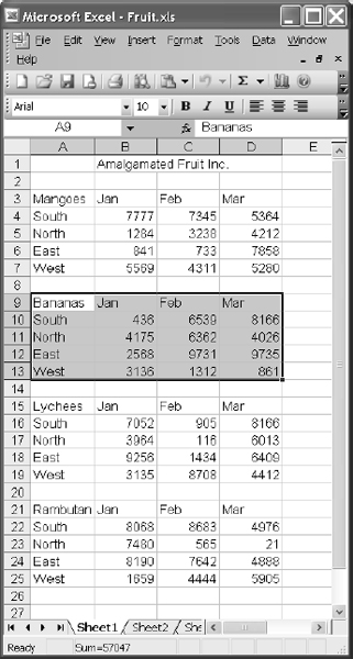
Figure 19-7

The same result can be achieved with the following code, given that cell A9 has been named Bananas:

Range(“Bananas”).CurrentRegion.Select

This property is very useful for tables that change size over time. You can select all the months up to the current month as the table grows during the year, without having to change the code each month. Naturally, in your code, there is rarely any need to select anything. If you want to perform a consolidation of the fruit figures into a single table in a sheet called Consolidation, and you have named the top-left corner of each table with the product name, you can use the following code:

Public Sub Consolidate()
  Dim Products As Variant
  Dim Source As Range
  Dim Destination As Range
  Dim i As Long

  Application.ScreenUpdating = False
  Products = Array(“Mangoes”, “Bananas”, “Lychees”, “Rambutan”)
  Set Destination = Worksheets(“Consolidation”).Range(“B4”)
  For i = LBound(Products) To UBound(Products)
    With Range(Products(i)).CurrentRegion
      Set Source = .Offset(1, 1).Resize(.Rows.Count - 1, .Columns.Count - 1)
    End With
    Source.Copy
    If i = LBound(Products) Then
      Destination.PasteSpecial xlPasteValues, xlPasteSpecialOperationNone
    Else
      Destination.PasteSpecial xlPasteValues, xlPasteSpecialOperationAdd
    End If
  Next i
  Application.CutCopyMode = False 'Clear the clipboard
End Sub

Figure 19-8 shows the output:

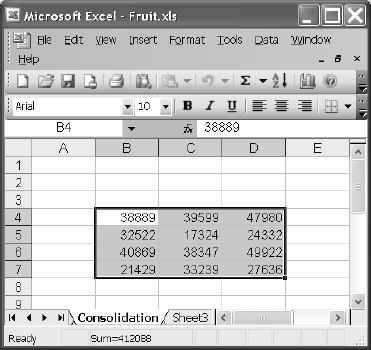
Figure 19-8

Screen updating is suppressed to cut out screen flicker and speed up the macro. The Array function is a convenient way to define relatively short lists of items to be processed. The LBound and UBound functions are used to avoid worrying about which Option Base has been set in the declarations section of the module. The code can be reused in other modules without a problem.

The first product is copied and its values are pasted over any existing values in the destination cells. The other products are copied and their values added to the destination cells. The clipboard is cleared at the end to prevent users accidentally carrying out another paste by pressing the Enter key.

End Property

The End property emulates the operation of Ctrl+Arrow key. If you have selected a cell at the top of a column of data, Ctrl+Down Arrow takes you to the next item of data in the column that is before an empty cell. If there are no empty cells in the column, you go to the last data item in the column. If the cell after the selected cell is empty, you jump to the next cell with data, if there is one, or the bottom of the worksheet.

The following code refers to the last data cell at the bottom of column A if there are no empty cells between it and A1:

Range(“A1”).End(xlDown)

To go in other directions, you use the constants xlUp, xlToLeft, and xlToRight.

If there are gaps in the data, and you want to refer to the last cell in column A, you can start from the bottom of the worksheet and go up, as long as data does not extend as far as A65536:

Range(“A6553 6”).End(xlUp)

In the section on rows, later in this chapter, you will see a way to avoid the A65536 reference and generalize the code above for different versions of Excel.

Referring to Ranges with End

You can refer to a range of cells from the active cell to the end of the same column with:

Range(ActiveCell, ActiveCell.End(xlDown)).Select

Say, you have a table of data, starting at cell B3, which is separated from the surrounding data by an empty row and an empty column. You can refer to the table, as long as it has continuous headings across the top and continuous data in the last column, using this line of code:

Range(“B3”, Range(“B3”).End(xlToRight).End(xlDown)).Select

The effect, in this case, is the same as using the CurrentRegion property, but End has many more uses as you will see in the following examples.

As usual, there is no need to select anything if you want to operate on a Range object in VBA. The following code copies the continuous headings across the top of Sheet1 to the top of Sheet2:

With Worksheets(“Sheet1”).Range(“A1”)
  .Range(.Cells(1), .End(xlToRight)).Copy Destination:= _
  Worksheets(“Sheet2”).Range(“A1”)
End With

This code can be executed, no matter what sheet is active, as long as the workbook is active.

Summing a Range

Suppose you want to place a SUM function in the active cell to add the values of the cells below it, down to the next empty cell. You can do that with the following code:

With ActiveCell
  Set aRange = Range(.Offset(1), .Offset(1).End(xlDown))
  .Formula = “=SUM(“ & aRange.Address & ”)”
End With

The Address property of the Range object returns an absolute address by default. If you want to be able to copy the formula to other cells and sum the data below them, you can change the address to a relative one and perform the copy as follows:

Public Sub SumRangeTest()
  Dim aRange As Range

  With ActiveCell
    Set aRange = Range(.Offset(1), .Offset(1).End(xlDown))
    .Formula = “=SUM(“ & aRange.Address(RowAbsolute:=False, _
      ColumnAbsolute:=False) & ”)”
    .Copy Destination:=Range(.Cells(1), .Offset(1).End(xlToRight).Offset(-1))
  End With
End Sub

The end of the destination range is determined by dropping down a row from the SUM, finding the last data column to the right, and popping back up a row.

Figure 19-9 shows the results:

Figure 19-9

Columns and Rows Properties

Columns and Rows are properties of the Application, Worksheet, and Range objects. They return a reference to all the columns or rows in a worksheet or range. In each case, the reference returned is a Range object, but this Range object has some odd characteristics that might make you think there are such things as a “Column object” and a “Row object”, which do not exist in Excel. They are useful when you want to count the number of rows or columns, or process all the rows or columns of a range.

Excel 97 increased the number of worksheet rows from the 16,384 in previous versions to 65,536. If you want to write code to detect the number of rows in the active sheet, you can use the Count property of Rows:

Rows.Count

This is useful if you need a macro that will work with all versions of Excel VBA, and detect the last row of data in a column, working from the bottom of the worksheet:

Cells(Rows.Count, “A”).End(xlUp).Select

If you have a multicolumn table of data in a range named SalesData, and you want to step through each row of the table making every cell in each row bold where the first cell is greater than 1000, you can use:

Public Sub BoldCells()
  Dim Row As Object
  For Each Row In Range(“SalesData”).Rows
    If Row.Cells(1).Value > 1000 Then
      Row.Font.Bold = True
    Else
      Row.Font.Bold = False
    End If
  Next Row

End Sub

This gives us the results shown in Figure 19-10:

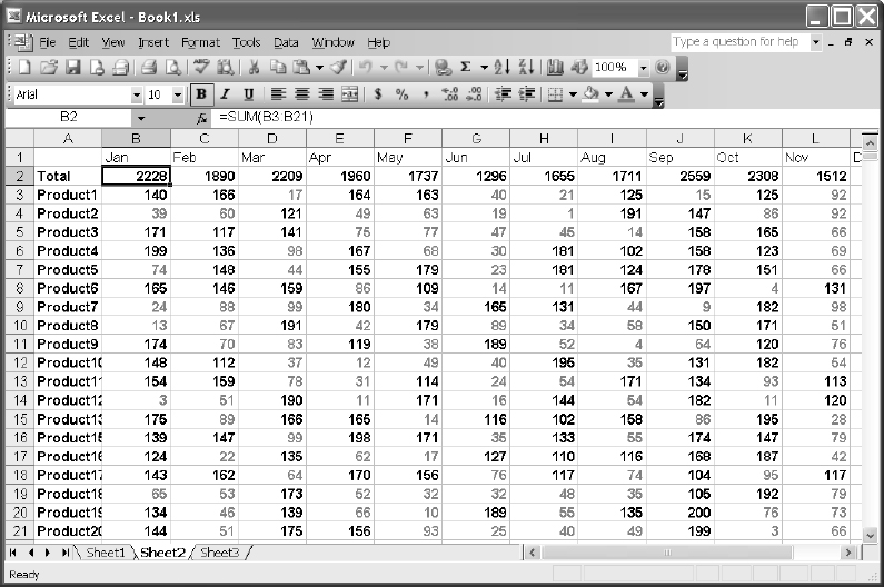
Figure 19-10

Curiously, you cannot replace Row.Cells(1) with Row(1), as you can with a normal Range object as it causes a runtime error. It seems that there is something special about the Range object referred to by the Rows and Columns properties. You may find it helps to think of them as Row and Column objects, even though such objects do not officially exist.

Areas

You need to be careful when using the Columns or Rows properties of non-contiguous ranges, such as those returned from the SpecialCells method when locating the numeric cells or blank cells in a worksheet, for example. Recall that a non-contiguous range consists of a number of separate rectangular blocks. If the cells are not all in one block, and you use the Rows.Count properties, you only count the rows from the first block. The following code generates an answer of 5, because only the first range, A1:B5, is evaluated:

Range(“A1:B5, C6:D10, E11:F15”).Rows.Count

The blocks in a non-contiguous range are Range objects contained within the Areas collection and can be processed separately. The following displays the address of each of the three blocks in the Range object, one at a time:

For Each aRange In Range(“A1:B5, C6:D10, E11:F15”).Areas
  MsgBox aRange.Address
Next Rng

The worksheet shown next contains sales estimates that have been entered as numbers. The cost figures are calculated by formulas. The following code copies all the numeric constants in the active sheet to blocks in Sheet3, leaving an empty row between each block:

Public Sub CopyAreas()
  Dim aRange As Range
  Dim Destination As Range

  Set Destination = Worksheets(“Sheet3”).Range(“A1”)
  For Each aRange In Cells.SpecialCells( _
    xlCellTypeConstants, xlNumbers).Areas

    aRange.Copy Destination:=Destination
    Set Destination = Destination.Offset(aRange.Rows.Count + 1)

  Next aRange
End Sub

This gives us the results in Figure 19-11 and Figure 19-12:

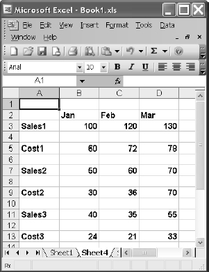
Figure 19-11

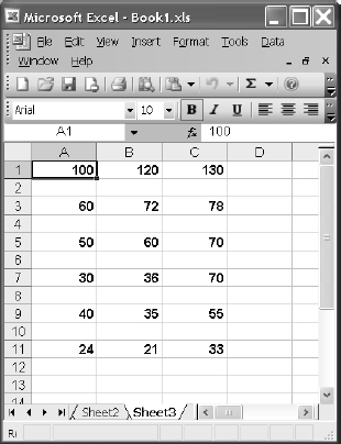
Figure 19-12

Union and Intersect Methods

Union and Intersect are methods of the Application object, but they can be used without preceding them with a reference to Application as they are members of <globals>. They can be very useful tools, as we shall see.

You use Union when you want to generate a range from two or more blocks of cells. You use Intersect when you want to find the cells that are common to two or more ranges, or in other words, where the ranges overlap. The following event procedure, entered in the module behind a worksheet, illustrates how you can apply the two methods to prevent a user selecting cells in two ranges B10:F20 and H10:L20. One use for this routine is to prevent a user from changing data in these two blocks:

Private Sub Worksheet_SelectionChange(ByVal Target As Range)
  Dim Forbidden As Range

  Set Forbidden = Union(Range(“B10:F20”), Range(“H10:L20”))
  If Intersect(Target, Forbidden) Is Nothing Then Exit Sub
  Range(“A1”).Select
  MsgBox “You can't select cells in ” & Forbidden.Address, vbCritical
End Sub

If you are not familiar with event procedures, refer to the Events section in Chapter 2. For more information on event procedures see Chapter 10.

The Worksheet_SelectionChange event procedure is triggered every time the user selects a new range in the worksheet associated with the module containing the event procedure. The preceding code uses the Union method to define a forbidden range consisting of the two non-contiguous ranges. It then uses the Intersect method, in the If test, to see if the Target range, which is the new user selection, is within the forbidden range. Intersect returns Nothing if there is no overlap and the Sub exits. If there is an overlap, the code in the two lines following the If test are executed—cell A1 is selected and a warning message is issued to the user.

Empty Cells

You have seen that if you want to step through a column or row of cells until you get to an empty cell, you can use the End property to detect the end of the block. Another way is to examine each cell, one at a time, in a loop structure and stop when you find an empty cell. You can test for an empty cell with the VBA IsEmpty function.

In the spreadsheet shown in Figure 19-13, you want to insert blank rows between each week to produce a report that is more readable.

Figure 19-13

The following macro compares dates, using the VBA Weekday function to get the day of the week as a number. By default, Sunday is day 1 and Saturday is day 7. If the macro finds today's day number is less than yesterday“s, it assumes a new week has started and inserts a blank row:

Public Sub ShowWeeks()
  Dim Today As Integer
  Dim Yesterday As Integer
  Range(“A2”).Select
  Yesterday = Weekday(ActiveCell.Value)
  Do Until IsEmpty(ActiveCell.Value)
    ActiveCell.Offset(1, 0).Select
    Today = Weekday(ActiveCell.Value)
    If Today < Yesterday Then
      ActiveCell.EntireRow.Insert

      ActiveCell.Offset(1, 0).Select
    End If
    Yesterday = Today
  Loop
End Sub

The result is shown in Figure 19-14.

Figure 19-14

Note that many users detect an empty cell by testing for a zero length string:

Do Until ActiveCell.Value = “”

This test works in most cases, and would have worked in the previous example, had we used it. However, problems can occur if you are testing cells that contain formulas that can produce zero length strings, such as the following:

=IF(B2=“Golieb”,“Trainee”,“”)

The zero length string test does not distinguish between an empty cell and a zero length string resulting from a formula. It is better practice to use the VBA IsEmpty function when testing for an empty cell.

Transferring Values between Arrays and Ranges

If you want to process all the data values in a range, it is much more efficient to assign the values to a VBA array and process the array rather than process the Range object itself. You can then assign the array back to the range.

You can assign the values in a range to an array very easily, as follows:

SalesData = Range(“A2:F10000”).Value

The transfer is very fast compared with stepping through the cells, one at a time. Note that this is quite different from creating an object variable referring to the range using

Set SalesData = Range(“A2:F10 000”)

When you assign range values to a variable such as SalesData, the variable must have a Variant data type. VBA copies all the values in the range to the variable, creating an array with two dimensions. The first dimension represents the rows and the second dimension represents the columns, so you can access the values by their row and column numbers in the array. To assign the value in the first row and second column of the array to Customer, use

Customer = SalesData(1, 2)

When the values in a range are assigned to a Variant, the indexes of the array that is created are always one-based, not zero-based, regardless of the Option Base setting in the declarations section of the module. Also, the array always has two dimensions, even if the range has only one row or one column. This preserves the inherent column and row structure of the worksheet in the array and is an advantage when you write the array back to the worksheet.

For example, if you assign the values in A1:A10 to SalesData, the first element is SalesData(1,1) and the last element is SalesData(10,1). If you assign the values in A1:E1 to SalesData, the first element is SalesData(1,1) and the last element is SalesData(1,5).

You might want a macro that sums all the Revenues for Golieb in our last example. The following macro uses the traditional method to directly test and sum the range of data:

Public Sub GoliebToAll()
  Dim Total As Double
  Dim i As Long
  With Range(“A2:G20”)
    For i = 1 To .Rows.Count
      If .Cells(i, 2) = “Golieb” Then Total = Total + .Cells(i, 7)
    Next i
  End With
  MsgBox “Golieb Total = ” & Format(Total, “$#,##0”)
End Sub

The following macro does the same job by first assigning the Range values to a Variant and processing the resulting array. The speed increase is very significant. It can be fifty times faster, which can be a great advantage if you are handling large ranges:

Public Sub GoliebTotal2()
  Dim SalesData As Variant
  Dim Total As Double
  Dim i As Long

  SalesData = Range(“A2:G20”).Value
  For i = 1 To UBound(SalesData, 1)
    If SalesData(i, 2) = “Golieb” Then Total = Total + SalesData(i, 7)
  Next i
  Call MsgBox(“Golieb Total = ” & Format(Total, “$#,##0”))
End Sub

You can also assign an array of values directly to a Range. Say, you want to place a list of numbers in column H of the FruitSales.xls example above, containing a 10 % discount on Revenue for customer Golieb only. The following macro, once again, assigns the range values to a Variant for processing:

Public Sub GoliebDiscount()
  Dim SalesData As Variant
  Dim Discount() As Variant
  Dim i As Long

  SalesData = Range(“A2:G20”).Value
  ReDim Discount(1 To UBound(SalesData, 1), 1 To 1)
  For i = 1 To UBound(SalesData, 1)
    If SalesData(i, 2) = “Golieb” Then
      Discount(i, 1) = SalesData(i, 7) * 0.1
    End If
  Next i
  Range(“H2”).Resize(UBound(SalesData, 1), 1).Value = Discount
End Sub

The code sets up a dynamic array called Discount, which it ReDims to the number of rows in SalesData and one column, so that it retains a two-dimensional structure like a range, even though there is only one column. After the values have been assigned to Discount, Discount is directly assigned to the range in column H. Note that it is necessary to specify the correct size of the range receiving the values, not just the first cell as in a worksheet copy operation.

The outcome of this operation is shown in Figure 19-15.

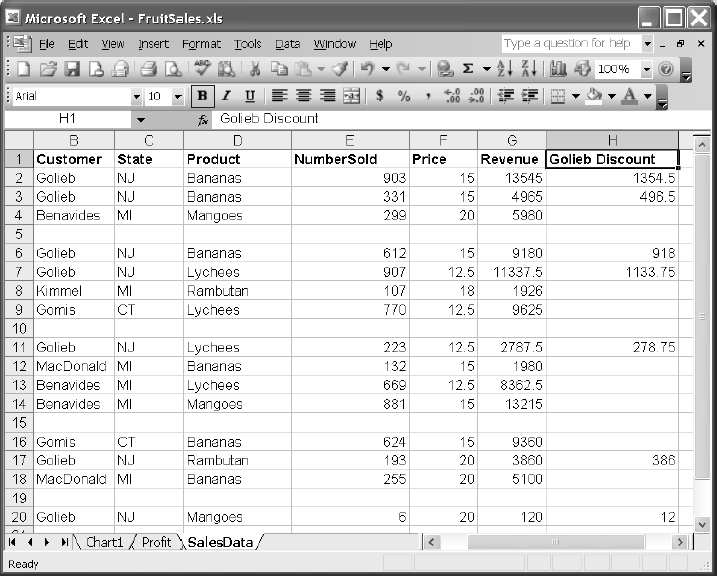
Figure 19-15

It is possible to use a one-dimensional array for Discount. However, if you assign the one-dimensional array to a range, it will be assumed to contain a row of data, not a column. It is possible to get around this by using the worksheet Transpose function when assigning the array to the range. Say, you have changed the dimensions of Discount as follows:

ReDim Discount(1 To Ubound(SalesData,1))

You could assign this version of Discount to a column with:

Range(“H2”).Resize(UBound(SalesData, 1), 1).Value = _
  WorkSheetFunction.Transpose(vaDiscount)

Deleting Rows

A commonly asked question is “What is the best way to delete rows that I do not need from a spreadsheet?” Generally, the requirement is to find the rows that have certain text in a given column and remove those rows. The best solution depends on how large the spreadsheet is and how many items are likely to be removed.

Say, that you want to remove all the rows that contain the text “Mangoes” in column D. One way to do this is to loop through all the rows, and test every cell in column D. If you do this, it is better to test the last row first and work up the worksheet row by row. This is more efficient because Excel does not have to move any rows up that would later be deleted, which would not be the case if you worked from the top down. Also, if you work from the top down, you can't use a simple For…Next loop counter to keep track of the row you are on because, as you delete rows, the counter and the row numbers no longer correspond:

Public Sub DeleteRows1()
  Dim i As Long
  Application.ScreenUpdating = False
  For i = Cells(Rows.Count, “D“).End(xlUp).Row To 1 Step -1
    If Cells(i, “D”).Value = “Mangoes” Then Cells(i, “D”).EntireRow.Delete
  Next i
End Sub

A good programming principle to follow is this: if there is an Excel spreadsheet technique you can utilize, it is likely to be more efficient than a VBA emulation of the same technique, such as the For…Next loop used here.

Excel VBA programmers, especially when they do not have a strong background in the user interface features of Excel, often fall into the trap of writing VBA code to perform tasks that Excel can handle already. For example, you can write a VBA procedure to work through a sorted list of items, inserting rows with subtotals. You can also use VBA to execute the Subtotal method of the Range object. The second method is much easier to code and it executes in a fraction of the time taken by the looping procedure.

However, it isn't always obvious which Excel technique is the best one to employ. A fairly obvious Excel contender to locate the cells to be deleted, without having to examine every row using VBA code, is the Edit → Find command. The following code uses the Find method to reduce the number of cycles spent in VBA loops:

Public Sub DeleteRows2()
  Dim FoundCell As Range
  Application.ScreenUpdating = False
  Set FoundCell = Range(“D:D”).Find(what:=“Mangoes”)
  Do Until FoundCell Is Nothing
    FoundCell.EntireRow.Delete
    Set FoundCell = Range(“D:D”).FindNext
  Loop
End Sub

This code is faster than the first procedure when there are not many rows to be deleted. As the percentage increases, it becomes less efficient. Perhaps we need to look for a better Excel technique.

The fastest way to delete rows, that we are aware of, is provided by Excel's AutoFilter feature:

Public Sub DeleteRows3()
  Dim LastRow As Long
  Dim aRange As Range

  Application.ScreenUpdating = False
  Rows(1).Insert
  Range(“D1”).Value = “Temp”
  With ActiveSheet
    .UsedRange
    LastRow = .Cells.SpecialCells(xlCellTypeLastCell).Row
    Set aRange = Range(“D1”, Cells(LastRow, “D”))
    aRange.AutoFilter Field:=1, Criteria1:=“Mangoes”
    aRange.SpecialCells(xlCellTypeVisible).EntireRow.Delete
    .UsedRange
  End With
End Sub

This is a bit more difficult to code, but it is significantly faster than the other methods, no matter how many rows are to be deleted. To use AutoFilter, you need to have field names at the top of your data. A dummy row is first inserted above the data and a dummy field name supplied for column D. The AutoFilter is only carried out on column D, which hides all the rows except those that have the text “Mangoes.”

The SpecialCells method is used to select only the visible cells in column D. This is extended to the entire visible rows and they are deleted, including the dummy field name row. The AutoFilter is automatically turned off when the dummy row is deleted.

Summary

In this chapter we have seen the most important properties and methods that can be used to manage ranges of cells in a worksheet. The emphasis has been on those techniques that are difficult or impossible to discover using the macro recorder. The properties and methods discussed were:

• Activate method
• Cells property
• Columns and Rows properties
• CurrentRegion property
• End property
• Offset property
• Range property
• Resize property
• Select method
• SpecialCells method
• Union and Intersect methods

We have also seen how to assign a worksheet range of values to a VBA array for efficient processing, and how to assign a VBA array of data to a worksheet range.

This chapter has also emphasized that it is very rarely necessary to select cells or activate worksheets, which the macro recorder invariably does as it can only record what we do manually. Activating cells and worksheets is a very time-consuming process and should be avoided if we want our code to run at maximum speed.

The final examples showed that it is usually best to utilize Excel's existing capabilities, tapping into the Excel object model, rather than write a VBA-coded equivalent. And bear in mind, some Excel techniques are better than others. Experimentation might be necessary to get the best code when speed is important.