CHAPTER 6
HETEROSCEDASTIC DATA
6.1 PREVIEW
The methodologies of Chapters 4 and 5 allow the measurement methods to have different variances, but they are assumed to remain constant over the range of values being measured. In other words, the measurements are assumed to be homoscedastic. In practice, however, a method’s variability often depends on the magnitude of measurement. This chapter is concerned with paired and unlinked repeated measurements data that exhibit such magnitude-dependent heteroscedasticity. We assume that the measurement methods have the same scale and extend the homoscedastic models of Chapters 4 and 5 to incorporate heteroscedasticity by letting the variances be functions of a suitably defined variance covariate. Two case studies illustrate this methodology.
6.2 INTRODUCTION
For homoscedastic data, the method comparison measures involve variances that are constant in that they do not depend on the values being measured. This assumption fails in many circumstances. In these cases, it is important to incorporate heteroscedasticity into the model. Otherwise, subsequent model-based inference on the measures may become unreliable. It may be possible to remove the heteroscedasticity altogether by a variance stabilizing transformation of data, such as the log transformation. Indeed, this transformation has been successful in removing the heteroscedasticity in vitamin D data (see Sections 1.13.3 and 4.4.3). But a transformation will not always be successful. Besides, a transformation other than the log is generally not recommended in method comparison studies because the differences of the transformed measurements may be difficult to interpret, rendering key agreement measures like TDI unusable. The VCF data in Exercises 1.10 and 6.9 provide an example where the log transformation is not quite successful in stabilizing the variance. Therefore, instead of attempting to remove the heteroscedasticity, we explicitly recognize it in the data modeling step as a function of the magnitude of measurement. This makes the method comparison measures that involve measurement’s variability change with the measurement’s magnitude.
As before, Yij, j = 1, 2, i = 1,...,n denote the paired measurements data with Yij as the measurement of the jth method on the ith subject. The Di = Yi2 − Yi1 denote the differences. Further, Yijk, k = 1,...,mij, j = 1, 2, i =1,...,n, denote the unlinked repeated measurements data with Yijk as the kth repeated measurement of the jth method on the ith subject. We do not consider linked repeated measurements data in this chapter; they are discussed in Chapter 8 in a more general setting. We assume that the methods have the same scale.
6.2.1 Diagnosing Heteroscedasticity
It is possible to diagnose heteroscedasticity by examining a trellis plot, a Bland-Altman plot, or even a scatterplot of the data. See Section 5.3 for how the latter two plots may be constructed for the repeated measurements data. Heteroscedasticity is observed in a trellis plot when the within-subject spread of points changes with the measurement level. It is evident in a Bland-Altman plot when points have a nonconstant vertical scatter. Heteroscedasticity is often easier to detect in a variant of the Bland-Altman plot where absolute values of centered differences , that is, ![]() , are plotted on the vertical axis instead of the Di themselves. One has to look for a trend in this plot, a simpler task than looking for a nonconstant scatter. A scatterplot also shows evidence of heteroscedasticity if the points have a nonconstant spread around the line or the curve that estimates the trend in the paired data.
, are plotted on the vertical axis instead of the Di themselves. One has to look for a trend in this plot, a simpler task than looking for a nonconstant scatter. A scatterplot also shows evidence of heteroscedasticity if the points have a nonconstant spread around the line or the curve that estimates the trend in the paired data.
With repeated measurements data, heteroscedasticity can also be diagnosed by examining plots of residuals obtained from fitting the homoscedastic mixed-effects model (5.1). A nonconstant vertical scatter in the plot of residuals against fitted values is suggestive of heteroscedasticity, and so is a trend in the plot of absolute residuals against the fitted values. The rationale behind these plots is that the expected value of the absolute value of a normal random variable with mean zero is a constant multiple of its standard deviation (Exercise 6.1). Therefore, if these plots show a trend, it indicates nonconstant variability. Although “residuals” may also be defined for paired measurements data following the homoscedastic bivariate normal model (4.6), their plots are generally not useful for diagnosing heteroscedasticity (see Section 6.5.2).
For both paired and repeated measurements data, one can also check for heteroscedasticity by conducting a test of null hypothesis of homoscedasticity. Such tests are provided later in this chapter.
6.2.2 Example Datasets
Below we introduce two datasets that will be used for case studies in this chapter. We revisit them in Sections 6.4.6 and 6.5.6.
6.2.2.1 Cyclosporin Data
Cyclosporin is an immunosuppressant drug widely used to prevent rejection of transplanted organs. This dataset consists of concentrations of cyclosporin (ng/mL) measured by assaying an aliquot of each of n = 56 blood samples from organ transplant recipients using two methods: high performance liquid chromatography (HPLC, method 1), the standard method, and an alternative radio-immunoassay (RIA, method 2). These are paired measurements data, ranging from 35 to 980 ng/mL. Figure 6.1 displays their trellis plot. It shows that the within-subject spread of the measurements tends to increase with concentration level. The Bland-Altman plot and its variant with absolute values of centered differences on the vertical axis are displayed in Figure 6.2. The heteroscedasticity is also evident in both the Bland-Altman plot where the vertical scatter appears to increase with average and its variant where an increasing trend is clear. All the three plots show an outlier.

Figure 6.1 Trellis plot of cyclosporin data.
6.2.2.2 Cholestero Data
These data come from a study in which two assays for serum cholesterol (mg/dL) are compared. One is Cobas Bio (method 1), a Centers for Disease Control standardized method that serves as the reference method. The other is Ektachem 700 (method 2), a laboratory analyzer that is treated as the test method. These assays are labeled as cobasb and echem, respectively. There are n = 100 subjects in the study. Serum cholesterol of every subject is measured ten times using each assay. Thus, these data have a balanced design and there is a total of M = 100 × 2 × 10 = 2000 observations. The repeated measurements are unlinked because a subject’s 20 measurements are obtained by subsampling the subject’s original blood sample. The measurements range from 45 to 372 mg/dL. Figure 6.3 displays their trellis plot. It clearly shows that the within-subject variations of both methods tend to increase with cholesterol level.

Figure 6.2 Plots for cyclosporin data. Panel (a): Bland-Altman plot with zero line. Panel (b): Plot of absolute values of centered differences against averages.
6.3 VARIANCE FUNCTION MODELS
We need a variance covariate v to account for heteroscedasticity of measurements. Let vi be the value of v for the ith subject. Since we would like to model variations of both measurement methods as functions of the magnitude of measurement, it is clear that the true measurement should be the covariate v. Note also that there is just one true value for each subject that both methods attempt to measure. Thus, this true value should be the common variance covariate for both methods. The measures of agreement will be functions of this covariate by definition, allowing us to evaluate how the extent of agreement changes with the magnitude of measurement.
A practical difficulty here is that the true values are not available in method comparison studies. We do, nevertheless, have error-free values of the methods, one from each method for every subject. (Recall from Section 1.3.1 that the true value of the subject and the error-free values of the methods are different quantities.) Let us denote the error-free values of the ith subject as µi1 for method 1 and µi2 for method 2. It is possible to model the variation for each method separately as a function of its own error-free value. But this will preclude us from evaluating agreement as a function of the magnitude of measurement, the common variance covariate. There are two obvious practical ways to get the common covariate as a function of the error-free values. One is to take vi = µi1 if there is an established method in the comparison serving as the reference, which if it exists, is taken to be method 1; otherwise, take vi = (µi1 + µi2)/2, the average of the two error-free values. Another is to take vi = (µi1 + µi2)/2 regardless of whether there is a reference in the comparison or not. More generally, we can think of the vi as a specified function of the error-free values,
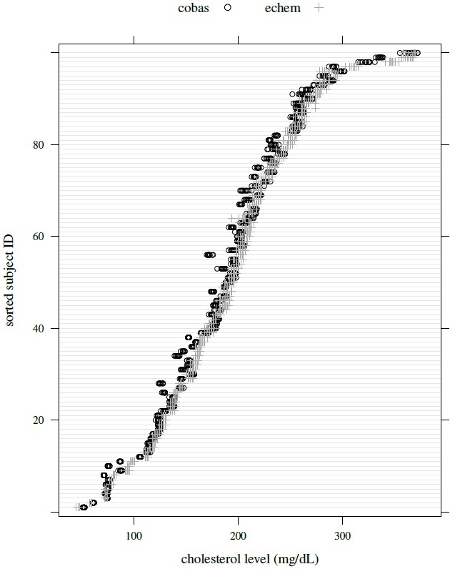
Figure 6.3 Trellis plot of cholesterol data.
 (6.1)
(6.1)denoting the magnitude of measurement for the purpose of modeling heteroscedasticity. The two vi defined earlier are special cases of this h function. The error-free values and hence the vi are unobservable random quantities. Generally they are non-negative as well.
Now that we have a working definition for the variance covariate v, we can define a variance function g(v, δ) that describes how the variation of a method changes with v and depends on a vector of heteroscedasticity parameters δ. More specifically, we will consider a model of the form σ2 g2(v, δ) for a variance. It may be noted that even though g is called a variance function, it is g2 that actually models the variance. The function g modeling the standard deviation is necessarily non-negative. We assume that g has a known parametric form and, for simplicity, take the heteroscedasticity parameter to be a scalar δ (see Section 8.3.2 for an example with a vector δ). The function g is continuous in δ, and is defined in a way to ensure that δ = 0 corresponds to homoscedasticity, that is, g(v, 0) = 1 for all v. Usually, it is also an increasing function in |v|.
We next introduce two simple, commonly used models for g. The first is the power model,
 (6.2)
(6.2)prescribing that g either increases or decreases as a power of the absolute value of the variance covariate. It increases in |v| if δ is positive and decreases in |v| if δ is negative. While the power δ may be any real number, large values for it in absolute value terms are rarely needed in practice. This model may not be appropriate if v can be zero or near zero because in this case the g function may also be zero or near zero, which may not be desirable. In particular, when v = 0, g is zero if δ > 0 and is undefined if δ < 0. If v ≠ 0, the power model for g is equivalent to assuming that the log of standard deviation is a linear function of log(|v|) with intercept log(σ) and slope δ.
The second is the exponential model,
 (6.3)
(6.3)Here both δ and v can be any real number, including zero. This model can also accommodate increasing and decreasing patterns of heteroscedasticity with v. In particular, if v ≥ 0 and δ > 0, which is commonly the case, the function increases exponentially in v. The exponential model is equivalent to assuming that the log of standard deviation is a linear function of v with intercept log(σ) and slope δ.
These models are obviously not exhaustive. However, it has been our experience that elaborate variance function models are generally not needed in method comparison studies. Our next task is to integrate the variance function models described here with the homoscedastic models of Chapters 4 and 5, yielding their heteroscedastic generalizations. We will first consider the repeated measurements data and then the paired measurements data.
6.4 REPEATED MEASUREMENTS DATA
In Chapter 5, under the assumption that the measurement methods have the same scale and the repeated measurements are unlinked, the data Yijk, k = 1,..., mij, j = 1, 2, i = 1,..., n, are modeled using the homoscedastic mixed-effects model (5.1). This model makes the usual normality and independence assumptions (see Section 5.4.1), including that
 (6.4)
(6.4)These errors are homoscedastic, that is, var(eijk) remains constant over the measurement range. From (5.1), the error-free values for methods 1 and 2 are, respectively,
 (6.5)
(6.5)6.4.1 A Heteroscedastic Mixed-Effects Model
To let the error variances of the methods depend on the magnitude of measurement, consider the variance covariate vi defined in (6.1). This vi is a known function h of the error-free values (µi1, µi2) given by (6.5). It serves as the magnitude of measurement and being a function of the random effects (bi, bi1, bi2), it is an unobservable random quantity. It also depends on the unknown intercept β0.
The homoscedasticity assumption for the errors can be relaxed by letting their variances depend on the variance covariate vi according to the variance function model
 (6.6)
(6.6)This model allows each method to have its own error variance function and heteroscedasticity parameter. But the covariate vi remains common to both methods. Notice that (6.6) models the error variances conditional on the random effects. The errors and the random effects are not independent anymore because the latter appear in the variance function through the covariate vi.
We obtain a heteroscedastic mixed-effects model by replacing the assumption (6.4) in the homoscedastic model (5.1) with the following assumption based on the variance function model in (6.6),
 (6.7)
(6.7)This model reduces to (5.1) when δ1 = δ2 = 0. It turns out that fitting this model poses computational difficulties (see Section 6.7). They arise from the fact that the random effects (bi, bi1, bi2) appear in the error variances through the covariate vi, preventing them from being explicitly averaged out to get a closed-form joint distribution for multiple measurements on a subject. This contrasts with the homoscedastic case where this distribution is multivariate normal.
One way to get around the computational difficulties is to approximate the variance covariate vi by replacing the unobservable error-free values (µi1, µi2) that determine it by their known, observable proxies, say, ![]() . The proxies are chosen so that they are free of the subject’s random effects and also are close to the error-free values. They are also held fixed during model fitting. This results in
. The proxies are chosen so that they are free of the subject’s random effects and also are close to the error-free values. They are also held fixed during model fitting. This results in
 (6.8)
(6.8)as the approximate variance covariate, and
 (6.9)
(6.9)as the corresponding variance function model. In contrast with (6.6), the ![]() here are fixed quantities, and the corresponding error variances are free of the random effects.
here are fixed quantities, and the corresponding error variances are free of the random effects.
Now, upon replacing the variance function model (6.6) with (6.9), we obtain a heteroscedastic mixed-effects model. This model is formulated as follows:
 (6.10)
k = 1,..., mij, j = 1, 2, i = 1,..., n, where
- the true values bi follow independent
 distributions,
 - the interactions bij follow independent N1(0, ψ2) distributions,
- for given
 , the random errors eijk follow independent
  distributions, and
 - bi, bij, and eijk are mutually independent.
This is the heteroscedastic model we will use for the repeated measurements data. The model (6.10) may be called “approximate” because the covariate ![]() involved herein is an approximation of the original variance covariate vi. For a fixed
involved herein is an approximation of the original variance covariate vi. For a fixed ![]() , the vectors of Mi = mi1 + mi2 measurements on subject i = 1,..., n follow independent Mi-variate normal distributions with means (Section 6.7 and Exercise 6.2)
, the vectors of Mi = mi1 + mi2 measurements on subject i = 1,..., n follow independent Mi-variate normal distributions with means (Section 6.7 and Exercise 6.2)
 (6.11)
and variances
 (6.12)
Further,
 (6.13)
is the common covariance between two replications of the same method, and
 (6.14)
is the common covariance between any two measurements from different methods on the same subject. Not surprisingly, the moments in (6.11)–(6.14) are identical to those in (5.2)–(5.5) derived for the homoscedastic model (5.1), with the obvious exception that the error variance ![]() has been replaced by
has been replaced by ![]() to incorporate heteroscedasticity. The unknown parameters in the model (6.10) are
to incorporate heteroscedasticity. The unknown parameters in the model (6.10) are ![]() . All inferences based on this model are made by holding the covariate
. All inferences based on this model are made by holding the covariate ![]() fixed. We will explain how to choose
fixed. We will explain how to choose ![]() and the variance functions gj in Section 6.4.2.
and the variance functions gj in Section 6.4.2.
Next, we need the distribution of the “typical” measurement pair (Y1, Y2) induced by the model (6.10). This distribution is used to derive the model-based measures of similarity, repeatability, and agreement later in Section 6.4.5. Due to heteroscedasticity, this distribution now depends on the variance covariate. Paralleling the development in Section 5.4.1, we get the distribution of (Y1, Y2) for a given value ![]() of the covariate as (Exercise 6.3)
of the covariate as (Exercise 6.3)
 (6.15)
In practice, V may be taken as the observed range of measurements. It follows that
 (6.16)
where
 (6.17)
6.4.2 Specifying the Variance Function
A key aspect of formulating the heteroscedastic model (6.10) is the specification of a model for the variance function in (6.9). This usually proceeds in three steps. First, we choose the proxies ![]() of the error-free values (µi1, µi2) that determine
of the error-free values (µi1, µi2) that determine ![]() through (6.8). By definition, the proxies need to be close to (µi1, µi2) while being free of the subject random effects. A simple choice is to take
through (6.8). By definition, the proxies need to be close to (µi1, µi2) while being free of the subject random effects. A simple choice is to take ![]() as the sample mean of the replicate measurements of the jth method on the ith subject, that is,
as the sample mean of the replicate measurements of the jth method on the ith subject, that is,
 (6.18)
It may be noted that ![]() . is a linear unbiased predictor of µij and satisfies
. is a linear unbiased predictor of µij and satisfies ![]() . The model (6.10) with (6.18) as
. The model (6.10) with (6.18) as ![]() can be fit by any statistical software capable of fitting heteroscedastic mixed-effects models with a known variance covariate.
can be fit by any statistical software capable of fitting heteroscedastic mixed-effects models with a known variance covariate.
An alternative possibility takes the BLUP of µij as ![]() (see Section 3.2.2). But the BLUPs themselves depend on unknown model parameters, calling for an iterative reweighting type of scheme for model fitting. It involves starting with an initial estimate of the model parameters, for example, using a homoscedastic fit, and cycling through the following steps until convergence:
(see Section 3.2.2). But the BLUPs themselves depend on unknown model parameters, calling for an iterative reweighting type of scheme for model fitting. It involves starting with an initial estimate of the model parameters, for example, using a homoscedastic fit, and cycling through the following steps until convergence:
- use the current parameter estimates to estimate the BLUPs,
- use the estimated BLUPs to compute the
 for an assumed h,
 - update the parameter estimates by fitting the heteroscedastic model, treating the as known.
Obviously, the choice of BLUP as ![]() makes the model fitting more computationally demanding than the previous alternative. But in our experience this additional cost does not pay off much in gaining higher accuracy of estimates (see Section 6.8 for a reference). Therefore, here we take the sample means
makes the model fitting more computationally demanding than the previous alternative. But in our experience this additional cost does not pay off much in gaining higher accuracy of estimates (see Section 6.8 for a reference). Therefore, here we take the sample means ![]() . in (6.18) as our
. in (6.18) as our ![]() .
.
The second step involves choosing the h function in (6.8) that determines the variance covariate ![]() . As we have settled on using
. As we have settled on using ![]() . as
. as ![]() , the two possibilities mentioned in Section 6.3 are
, the two possibilities mentioned in Section 6.3 are
 (6.19)
and
 (6.20)
regardless of whether or not there exists a reference method. The two alternatives differ only when a reference method is present in the comparison. But even this distinction between them is not critical as the two tend to yield similar model fits. Nevertheless, here we work with the average (6.20) for the sake of concreteness. Note that the h function may also be a transformation of this average, for example, the log transformation.
The third step consists of choosing the actual variance functions gj in (6.9). We are only interested in determining the forms of these functions; the coefficients involved in them constitute the unknown heteroscedasticity parameters δj that are estimated by the ML method together with all other model parameters. One way to come up with the desired functions is to fit the homoscedastic model (5.1) to the data, get the residuals, and analyze the absolute values of the residuals using ordinary regression. Under the model, these residuals are approximately normally distributed with mean zero, implying that the mean of the absolute residuals is approximately ![]() times the standard deviations of the residuals (Exercise 6.1). These standard deviations in turn approximate the error standard deviations, which are precisely the functions gj defined in (6.9) up to a multiplicative constant. This means we can determine the forms of the gj functions by examining the trends in absolute residuals as a function of the variance covariate
times the standard deviations of the residuals (Exercise 6.1). These standard deviations in turn approximate the error standard deviations, which are precisely the functions gj defined in (6.9) up to a multiplicative constant. This means we can determine the forms of the gj functions by examining the trends in absolute residuals as a function of the variance covariate ![]() using ordinary regression techniques. For this, one may proceed as follows:
using ordinary regression techniques. For this, one may proceed as follows:
- Plot the absolute residuals against for each method. Also plot the log of the absolute residuals against both and log(||).
- Examine the trends in these scatterplots. Fit simple parametric functions, for example, linear or log-linear functions, via ordinary regression to describe the trends; superimpose the fitted curves on the scatterplots; and visually judge which functions provide the most reasonable fit. Take this function for the jth method as gj, with coefficients in the function treated as unknown parameters. Consider simple linear regression fits of log of absolute residuals on either , for the exponential model, or log(||), for the power model (see Section 6.3). The two methods may have altogether different gj functions. Moreover, one may have more than one candidate for a gj function.
6.4.3 Model Fitting and Evaluation
The model (6.10) treats the variance covariate ![]() as a known quantity that is held fixed during model fitting. Therefore, the model can be fit by the ML method using any mixed-effects model fitting software that can handle heteroscedasticity of errors in terms of known variance covariates. As before, upon fitting the model we get
as a known quantity that is held fixed during model fitting. Therefore, the model can be fit by the ML method using any mixed-effects model fitting software that can handle heteroscedasticity of errors in terms of known variance covariates. As before, upon fitting the model we get

as the ML estimates of model parameters; ![]() as the predicted values of the random effects;
as the predicted values of the random effects;

as the fitted values; ![]() as the residuals; and
as the residuals; and

as the standardized residuals. When the heteroscedastic model (6.10) holds, these standardized residuals are approximately distributed as independent draws from a standard normal distribution. One can use these quantities to perform model diagnostics as described in Section 3.2.4 to validate the mixed-effects model assumptions.
Of particular interest is the adequacy of the assumed variance functions models. Obviously, if the residual plots for both methods pass the diagnostics, then the assumed gj can be deemed adequate. Alternatively, if the number of replications mij is large enough for the sample standard deviations of measurements to be stable for each (i, j), then this adequacy can be judged directly. For this, one can examine the plot of the subject-specific sample standard deviations against ![]() , separately for each method, superimposed with the model-based fitted error standard deviation curves. The latter are obtained by taking the square root of (6.9) and replacing the unknown parameters by their ML estimates. Naturally, if the assumed gj functions do not fit well, one has to return to the step where absolute residuals from the homoscedastic model fit are analyzed by regression to come up with an alternative model that may provide a better fit. On the other hand, if there is more than one candidate model for the gj functions then this adequacy checking can be repeated for each candidate to find the best fitting model with a natural preference for a simpler model.
, separately for each method, superimposed with the model-based fitted error standard deviation curves. The latter are obtained by taking the square root of (6.9) and replacing the unknown parameters by their ML estimates. Naturally, if the assumed gj functions do not fit well, one has to return to the step where absolute residuals from the homoscedastic model fit are analyzed by regression to come up with an alternative model that may provide a better fit. On the other hand, if there is more than one candidate model for the gj functions then this adequacy checking can be repeated for each candidate to find the best fitting model with a natural preference for a simpler model.
6.4.4 Testing for Homoscedasticity
In applications, we need to supplement the visual assessment of the need for a heteroscedastic model by testing the null hypothesis of homoscedasticity,
 (6.21)
A likelihood ratio test can be used for this purpose. This involves fitting both the heteroscedastic model (6.10) and the homoscedastic model (5.1) that results when the null hypothesis is true. From (3.32), the likelihood ratio statistic is
 (6.22)
where L1 and L2 are the maximum likelihoods under the models (5.1) and (6.10), respectively. Following Section 3.3.7, the p-value for testing H0 can be approximated by the probability on the right of the observed value of the statistic under a χ2 distribution with two degrees of freedom. The homoscedastic and heteroscedastic models can also be compared using model selection criteria such as AIC and BIC (Section 3.3.7). These can also be used to distinguish between multiple candidate models for the variance functions.
6.4.5 Evaluation of Similarity, Agreement, and Repeatability
We follow Sections 5.5 and 5.6 and adapt the methodology for evaluation of similarity, agreement, and repeatability developed there to handle the heteroscedastic model (6.10). The evaluation involves examining two-sided confidence intervals for measures of similarity and one-sided confidence bounds for measures of agreement and repeatability. When a measure depends on ![]() , we get its pointwise confidence band over V. A simultaneous confidence band over a grid in V can also be constructed (see Section 3.3.5).
, we get its pointwise confidence band over V. A simultaneous confidence band over a grid in V can also be constructed (see Section 3.3.5).
Our task is to derive the various measures, focusing initially on the measures of similarity and agreement. Upon comparing the distributions of the “typical” measurement pair (Y1, Y2) that are used to develop these measures, we find that (6.15) is the same as (5.7) except that ![]() is replaced by
is replaced by ![]() . It follows that the same replacement in the measures based on (5.7) would give their heteroscedastic counterparts that are based on (6.15). The counterparts that involve the error variances are now functions of the variance covariate
. It follows that the same replacement in the measures based on (5.7) would give their heteroscedastic counterparts that are based on (6.15). The counterparts that involve the error variances are now functions of the variance covariate ![]() .
.
The two measures of similarity considered in Section 5.5 are the fixed intercept β0 and the precision ratio λ. The first remains the same and the heteroscedastic version of the second is
 (6.23)
The measures of agreement considered in Section 5.5 are the CCC and TDI. Using (5.19) and (5.21), we obtain
 (6.24)
and
 (6.25)
where τ2(![]() ) is given
) is given ![]() in (6.17).
in (6.17).
Consider next the measures of repeatability discussed in Section 5.6. These are derived from the distributions of (Yj, ![]() ) , where
) , where ![]() is a replication of Yj, j = 1, 2. Not surprisingly, these distributions under the heteroscedastic model (6.10) are the same as those given by (5.24) and (5.25) under the homoscedastic model (5.1) with the exception that
is a replication of Yj, j = 1, 2. Not surprisingly, these distributions under the heteroscedastic model (6.10) are the same as those given by (5.24) and (5.25) under the homoscedastic model (5.1) with the exception that![]() is replaced by
is replaced by ![]() (Exercise 6.4). The same replacement in the repeatability measures in (5.27) gives the heteroscedastic versions of CCCj and TDIj as
(Exercise 6.4). The same replacement in the repeatability measures in (5.27) gives the heteroscedastic versions of CCCj and TDIj as
 (6.26)
The heteroscedastic version of 95 % limits of agreement can be obtained from (5.22) as
 (6.27)
with ![]() denoting the ML estimator of τ2(
denoting the ML estimator of τ2(![]() ) given by (6.17); and its repeatability analogs can be obtained from (5.28) as
) given by (6.17); and its repeatability analogs can be obtained from (5.28) as
 (6.28)
6.4.6 Case Study: Cholesterol Data
These data, introduced in Section 6.2.2.2, consist of measurements of serum cholesterol (in mg/dL) obtained using Cobas Bio (method 1) and Ektachem assays (method 2) from n = 100 subjects. The data have a balanced design with m = 10 unlinked replications. Their trellis plot is displayed in Figure 6.3. Although considerable overlap is seen between the values of the two assays, it is also apparent that the Ektachem measurements tend to be larger and have higher within-subject variation than the Cobas Bio measurements. Moreover, for both assays, this variation seems to increase with the cholesterol level, implying magnitude-dependent heteroscedasticity. The within-subject variation remains substantially lower than the between-subject variation. There is also evidence of assay × subject interaction as the average difference between the assays does not appear constant over the subjects. Figure 6.4 shows scatterplots and Bland-Altman plots for these data based on both randomly formed measurement pairs (top panel) and averages over the replications (bottom panels). The two panels look nearly the same. The scatterplots show high correlation between the assays. The Bland-Altman plots are not centered at zero, suggesting a difference in fixed biases of the assays, but there is no trend in the plots, suggesting a common scale for the assays.

Figure 6.4 Plots for cholesterol data. Top panel (left to right): Scatterplot with line of equality and Bland-Altman plot with zero line based on 100 randomly formed measurement pairs. Bottom panel (left to right): Same as top panel but based on average measurements.
A distinguishing feature of these data, apparent from the trellis plot, is that it exhibits magnitude-dependent heteroscedasticity. To examine it further, we fit the homoscedastic mixed-effects model (5.1) and get the standardized residuals. In Figure 6.5, we plot them as well as their absolute values against the fitted values separately for each assay. The fan-shaped pattern in both residual plots confirms that the error variations of both assays increase with the magnitude of measurement. The increasing trends in both absolute residual plots lead to the same conclusion.
To fit the heteroscedastic model (6.10), we need to come up with models for the error variance functions of the two assays. From the discussion in Section 6.4.2, we take the average (6.20) as the variance covariate ![]() . As this is a positive quantity, there is no need to take its absolute value in the variance functions. Figure 6.6 displays plots of log of absolute values of residuals from the homoscedastic fit against both log(
. As this is a positive quantity, there is no need to take its absolute value in the variance functions. Figure 6.6 displays plots of log of absolute values of residuals from the homoscedastic fit against both log(![]() ) and
) and ![]() . These scatterplots are superimposed with fitted regression lines. It is apparent that the trend in each plot can be approximated by a straight line, at least as our first approximation. This suggests that both the power model (6.2) and the exponential model (6.3) seem reasonable choices for the variance function model. In addition, models of the same form can be used for both methods.
. These scatterplots are superimposed with fitted regression lines. It is apparent that the trend in each plot can be approximated by a straight line, at least as our first approximation. This suggests that both the power model (6.2) and the exponential model (6.3) seem reasonable choices for the variance function model. In addition, models of the same form can be used for both methods.

Figure 6.5 Plots of standardized residuals (top panel) and their absolute values (bottom panel) against fitted values from a homoscedastic fit to cholesterol data.

Figure 6.6 Plots of log of absolute residuals from a homoscedastic fit to cholesterol data against log( ) (top panel) and (bottom panel) with as the average cholesterol level of a subject. A simple linear regression fit is superimposed on each plot.
Motivated by this finding, we first fit the heteroscedastic mixed-effects model (6.10) with the power variance function model, that is,

for both assays. The resulting residual plot is shown in Figure 6.7. The residuals are centered at zero and their vertical scatter appears constant, suggesting that the power model is successful in explaining the heteroscedasticity in the data. However, the same is true for the exponential model as well (Exercise 6.5). Unable to distinguish between the two models on the basis of the residual plots alone, we turn to comparing the observed and the fitted within-subject standard deviations from the two models. Recall that m = 10 replications are available at each subject-method combination, enough to provide reasonably stable observed standard deviations. Figure 6.8 displays the observed and the fitted values. The fitted standard deviations from the power model for both assays appear linear because the estimated δ1 and δ2 are practically 1 (see Table 6.1). It is clear that both models provide comparable fits except near the right end of the measurement range where the power model appears to fit better than the exponential model. The two models can be further compared using the model comparison criteria AIC and BIC (Section 3.3.7). Their respective values are 9753 and 9798 for the power model, and 9767 and 9812 for the exponential model. Both criteria favor the power model as their values in this case are smaller than the exponential model. (The likelihood ratio test cannot be used to compare the two models because they are not nested.)

Figure 6.7 Residual plots from a heteroscedastic fit to cholesterol data using power variance function models.
Further diagnostics for the power model, including the assessment of normality of random effects and errors, show some evidence of heavy tails for the residuals, but otherwise the fit is reasonably good (Exercise 6.5). This is not of serious concern, as in our experience, the overall conclusions of a method comparison data analysis based on mixed-effects models tend to be robust against error distributions with moderately heavy tails. Therefore, the power model is assumed for the rest of the analysis.
Figure 6.8 Observed versus fitted within-subject standard deviations from power (solid line) and exponential (broken curve) variance function models for cholesterol data. The covariate  , the subject average, is plotted on the horizontal axis. The observed values are represented by the points and the fitted values are represented by the curves.
Table 6.1 presents estimates of the eight parameters in the model, their standard errors, and the 95% confidence intervals. Even though there is clear evidence of heteroscedasticity, it is useful nevertheless to test the null hypothesis of homoscedasticity, δ1 = δ2 = 0. The log-likelihood for the fitted power model is −4868.6 and it is −5117.6 for the homoscedastic model (5.1) that corresponds to the null hypothesis. Thus, the value of the likelihood ratio statistic (6.22) is 2{−4868.6 −(−5117.6)} = 498. The p-value for this test is practically zero, leading, as expected, to a strong rejection of the homoscedasticity hypothesis.
Table 6.1 Summary of parameter estimates for cholesterol data. Methods 1 and 2 refer to Cobas Bio and Ektachem, respectively.
| Parameter | Estimate | SE | 95% Interval |
| β0 | 5.58 | 0.74 | (4.14, 7.02) |
| µb | 184.38 | 6.60 | (171.45, 197.31) |
| log( |
8.37 | 0.14 | (8.09, 8.65) |
| log(ψ2) | 3.28 | 0.14 | (3.00, 3.56) |
| −9.43 | 0.57 | (−10.55, −8.31) | |
| −8.49 | 0.59 | (−9.64, −7.34) | |
| δ1 | 1.02 | 0.06 | (0.91, 1.12) |
| δ2 | 0.98 | 0.06 | (0.86, 1.09) |
We substitute the ML estimates from Table 6.1 in (6.15) and (6.16) to obtain the fitted distribution of (Y1, Y2) given the cholesterol level ![]() as
as

and of D given ![]() as
as
 (6.29)
From Exercise 6.4, a similar substitution gives the fitted distributions of the intra-method differences Dj given ![]() . It follows that
. It follows that
 (6.30)
The range of ![]() is taken to be V = (45, 372), the observed measurement range. These distributions confirm several of our findings based on the various plots. In particular, the Cobas Bio assay has a smaller estimated mean and a smaller estimated error standard deviation than Ektachem. Cobas Bio’s error standard deviation, {(8.0 × 10⁻⁵)
is taken to be V = (45, 372), the observed measurement range. These distributions confirm several of our findings based on the various plots. In particular, the Cobas Bio assay has a smaller estimated mean and a smaller estimated error standard deviation than Ektachem. Cobas Bio’s error standard deviation, {(8.0 × 10⁻⁵)![]() 2.03}1/2, increases from 0.59 to 4.62, whereas that of Ektachem, {(2.06 × 10⁻⁴)
2.03}1/2, increases from 0.59 to 4.62, whereas that of Ektachem, {(2.06 × 10⁻⁴)![]() 1.95}1/2, increases from 0.43 to 3.65. Both the error standard deviations are completely dominated by the between-subject standard deviation as measured by
1.95}1/2, increases from 0.43 to 3.65. Both the error standard deviations are completely dominated by the between-subject standard deviation as measured by ![]() It is then not surprising that the overall standard deviations of both assays are nearly a constant around 66. Besides, the correlation between the assays is extremely high—around 0.99 throughout the range. The effect of nonconstant error variation is somewhat more apparent in the standard deviation of D; it increases from 7.32 to 9.37. Note from (6.17) that there are two components of variation in D—one due to the errors and the other due to subject × method interactions, a component of the between-subject variation. While the latter remains a constant, it dominates the former, making the standard deviation of D depend mildly on the magnitude of measurement.
It is then not surprising that the overall standard deviations of both assays are nearly a constant around 66. Besides, the correlation between the assays is extremely high—around 0.99 throughout the range. The effect of nonconstant error variation is somewhat more apparent in the standard deviation of D; it increases from 7.32 to 9.37. Note from (6.17) that there are two components of variation in D—one due to the errors and the other due to subject × method interactions, a component of the between-subject variation. While the latter remains a constant, it dominates the former, making the standard deviation of D depend mildly on the magnitude of measurement.
Figure 6.9 plots the 95% limits of agreement for measurements between and within the methods. They are computed from (6.27) and (6.28), respectively. By definition, the inter-method limits are centered at ![]() and the intra-method limits for both methods are centered at zero. The effect of error heteroscedasticity is clearly apparent in the intra-method limits but less so in the inter-method limits. This discrepancy occurs because the former limits are solely determined by the error variation, whereas the latter limits depend on the variation of D wherein the variation of the errors is dominated by that of the subject × method interactions.
and the intra-method limits for both methods are centered at zero. The effect of error heteroscedasticity is clearly apparent in the intra-method limits but less so in the inter-method limits. This discrepancy occurs because the former limits are solely determined by the error variation, whereas the latter limits depend on the variation of D wherein the variation of the errors is dominated by that of the subject × method interactions.
Next, we examine similarity of the two assays. From Table 6.1, the 95% confidence interval for β0 is (4.15, 7.02). The entire interval is above zero. Recalling that β0 represents the difference in means of the two assays under the equal scales assumption, this implies larger mean for Ektachem. Panel (a) of Figure 6.10 displays the estimate and two-sided 95% pointwise confidence band for the precision ratio λ(![]() ) as a function of the cholesterol level. This measure is defined in (6.23). The entire band lies below one, leading to the conclusion that Cobas Bio is more precise than Ektachem. The estimated λ suggests that the former is about 40% more precise than the latter. On the whole, the two assays cannot be considered similar. Cobas Bio is clearly superior to Ektachem because of its higher precision. These findings are consistent with what we saw earlier in the plots.
) as a function of the cholesterol level. This measure is defined in (6.23). The entire band lies below one, leading to the conclusion that Cobas Bio is more precise than Ektachem. The estimated λ suggests that the former is about 40% more precise than the latter. On the whole, the two assays cannot be considered similar. Cobas Bio is clearly superior to Ektachem because of its higher precision. These findings are consistent with what we saw earlier in the plots.

Figure 6.9 95% limits of inter- and intra-method agreement for cholesterol data as a function of magnitude of measurement. The inter-method limits, based on the distribution of D, are centered at 5.58. The intra-method limits, based on the distributions of D1 and D2, are centered at zero.
For evaluation of repeatability, panel (b) of Figure 6.10 presents one-sided 95% pointwise lower confidence bands for intra-method versions of CCC. Also presented in panel (c) of the figure are one-sided 95% pointwise upper confidence bands for the intra-method versions of TDI (0.90) and their reflections over a horizontal line at zero. These repeatability measures are defined in (6.26). We see that the CCC lower band for Cobas Bio is entirely above that of Ektachem and the converse is true for the TDI upper bands. This indicates that Cobas Bio has higher intra-method agreement than Ektachem. This conclusion is expected as our evaluation of similarity just showed that Cobas Bio has smaller error variation. More noteworthy is the fact that the CCC bands decrease and the TDI bands increase as the cholesterol level increases. This means that the extent of intra-method agreement for both assays becomes progressively worse as the magnitude of measurement increases. The intra-method CCC lower bands remain above 0.99 throughout the measurement range, implying that the CCC estimates clearly exceed 0.99. Because these are estimated reliabilities of the assays, such larges values essentially reflect that the within-subject variations for both assays are very small compared to the between-subject variation. The TDI bounds increase from 1 to about 9 for Cobas Bio and to about 12 for Ektachem as the cholesterol level increases from 45 to 372. The value of 12, for example, implies that, when the true cholesterol value is 372, 90% of the time the difference between two replications of Ektachem on the same subject falls within ±12. The TDI bounds are only about 2-3% of the magnitude of measurement, indicating a high degree of intra-method agreement for both assays.

Figure 6.10 Plots for cholesterol data. (a) Estimate (solid curve) and 95% pointwise two-sided confidence band (broken curves) for precision ratio; (b) 95% lower confidence bands for inter- and intra-method versions of CCC; (c) 95% upper confidence bands for inter- and intra-method versions of TDI (0.90) as well as their reflections around the horizontal line at zero, giving the corresponding pointwise tolerance bands; and (d) same as panel (c) but with Ektachem recalibrated to have the same estimated mean as Cobas Bio.
Panels (b) and (c) of Figure 6.10 also present one-sided 95% pointwise confidence bands for CCC and TDI (0.90) for evaluation of agreement between the assays. Just like their intra-method counterparts, the CCC lower band decreases and the TDI upper band increases as the cholesterol level increases. Thus, in an absolute sense, the extent of agreement between the assays becomes progressively worse, albeit only by a small amount, with increasing cholesterol levels. The CCC lower bounds range between 0.982 and 0.987, suggesting excellent agreement between the assays over the entire measurement range. But this conclusion may be misleading because the between-subject variation in these data overwhelms the within-subject variation. A better view of agreement is given by the TDI whose estimate increases from 15.1 to 17.9 and upper bound increases from 17 to 19.5 as the cholesterol level increases from 45 to 372. For example, the bound of 17 shows that 90% of differences in measurements from the assays fall within ±17 when the true value is 45. Such a difference is unacceptably large relative to the true value. On the other hand, a difference as large as ±19.5 may be acceptable when the true value is 372. The bounds of 17 and 19.5 are, respectively, about 38% and 5% of the true value. It follows that we may conclude satisfactory agreement between the assays for large cholesterol values but not for very small values.
The similarity evaluation reveals that a difference in the means of the assays is a contributor to disagreement. Recalibration of Ektachem by subtracting ![]() from its measurements makes the mean difference zero, but it improves the extent of agreement only slightly. The TDI bounds now range from 13.5 to 16.5 instead of 17 to 19.5 (compare panels (c) and (d) of Figure 6.10). The CCC bounds increase only slightly as they were already close to 1 (not shown).
from its measurements makes the mean difference zero, but it improves the extent of agreement only slightly. The TDI bounds now range from 13.5 to 16.5 instead of 17 to 19.5 (compare panels (c) and (d) of Figure 6.10). The CCC bounds increase only slightly as they were already close to 1 (not shown).
Taken together, we find that the assays exhibit high intra-method agreement throughout the measurement range, especially at the low end of the range. But their inter-method agreement, although potentially satisfactory for the upper half of the measurement range, cannot be considered satisfactory at the low end. Even the recalibration of Ektachem does not help matters much. Thus, the assays cannot be used interchangeably. Cobas Bio remains the superior of the two assays because of its higher precision. The apparent mismatch in the conclusions regarding inter- and intra-method agreement can be explained by the fact that the variation in the errors is rather small while the variation in the subject × method interactions is relatively large. This results in small variation in D1 and D2 but not in D when considered relative to the true value—see (6.29) and (6.30). The relative variation is especially large at the low end of measurements. It also follows from this discussion that any further improvement in the extent of inter-method agreement would primarily involve reducing the interaction variation. This may not be a simple task.
It may be of interest to ask how the results would compare if the heteroscedasticity in the data is ignored and they are analyzed assuming the homoscedastic model (5.1). This is explored in Exercise 6.5. It turns out that the overall conclusions regarding similarity and repeatability are similar to the heteroscedastic case, with the obvious exception that these measures do not depend on the cholesterol value anymore. In addition, there is virtually no change in the inference on CCC as its 95% lower confidence bound is now 0.985, as opposed to ranging over 0.982 to 0.987 in the heteroscedastic case. The estimate of TDI (0.90) is 16 and its 95% upper confidence bound is 17.6. The bound of 17.6 is not terribly far from either endpoint of the interval (17, 19.5) over which the heteroscedastic bound ranges (Figure 6.10, panel (c)). This is primarily because the effect of the error variation, the only entity that depends on the magnitude of measurement, is dominated by the between-subject variation. If this were not the case, the effect of heteroscedasticity on the overall conclusions would have been more prominent. In any case, it is clear that not taking account of heteroscedasticity leads to underestimation of the extent of agreement for small cholesterol levels and its overestimation for large ones.
Finally, recall that we chose the average in (6.20) as the variance covariate ![]() for modeling heteroscedasticity. We leave it for the reader to verify that choosing instead the average of either only the reference method measurements or all the measurements on the ith subject as the
for modeling heteroscedasticity. We leave it for the reader to verify that choosing instead the average of either only the reference method measurements or all the measurements on the ith subject as the ![]() does not alter the results in any significant manner (Exercise 6.5).
does not alter the results in any significant manner (Exercise 6.5).
6.5 PAIRED MEASUREMENTS DATA
In the previous section, replications of each measurement allowed us to model within-subject variations of the methods as functions of a variance covariate ![]() that served as a proxy for the magnitude of measurement. We then replaced the constant error variances in the homoscedastic mixed-effects model with variance function models to get a heteroscedastic model for the data. In principle, a similar approach can be used with the paired measurements data. It would model the error variations in the homoscedastic mixed-effects model (4.1) by variance function models. But this does not work in practice because the paired data do not have enough information to reliably estimate even the error variances in the homoscedastic model. Any addition of further parameters to model error heteroscedasticity will only make the matters worse. A more viable alternative in Chapter 4 was to model the data Yij, j = 1, 2, i = 1,..., n as a random sample of (Y1, Y2) following the bivariate normal distribution specified in (4.6). In particular, this model assumes that
that served as a proxy for the magnitude of measurement. We then replaced the constant error variances in the homoscedastic mixed-effects model with variance function models to get a heteroscedastic model for the data. In principle, a similar approach can be used with the paired measurements data. It would model the error variations in the homoscedastic mixed-effects model (4.1) by variance function models. But this does not work in practice because the paired data do not have enough information to reliably estimate even the error variances in the homoscedastic model. Any addition of further parameters to model error heteroscedasticity will only make the matters worse. A more viable alternative in Chapter 4 was to model the data Yij, j = 1, 2, i = 1,..., n as a random sample of (Y1, Y2) following the bivariate normal distribution specified in (4.6). In particular, this model assumes that
 (6.31)
This model can be extended by directly letting these measurement variances, not the error variances of the methods, depend on the variance covariate ![]() through variance function models. We now provide the relevant details by paralleling the development of the previous section.
through variance function models. We now provide the relevant details by paralleling the development of the previous section.
6.5.1 A Heteroscedastic Bivariate Normal Model
Let the variances of the measurement methods depend on a given value ![]() of the variance covariate as
of the variance covariate as
 (6.32)
Here gj is a variance function with heteroscedasticity parameter δj (Section 6.3), and ![]() Replacing the variances (6.31) in the bivariate normal model (4.6) with their heteroscedastic counterparts (6.32) gives the distribution of (Y1, Y2) given
Replacing the variances (6.31) in the bivariate normal model (4.6) with their heteroscedastic counterparts (6.32) gives the distribution of (Y1, Y2) given ![]() as
as
 (6.33)
where
 (6.34)
Notice that the covariance of this distribution depends on ![]() in such a way that the correlation ρ remains constant. This contrasts with the heteroscedastic model of previous section in which the covariance remained constant whereas the correlation depended on
in such a way that the correlation ρ remains constant. This contrasts with the heteroscedastic model of previous section in which the covariance remained constant whereas the correlation depended on ![]() , see (6.15). This switch is done for computational ease in model fitting (see Section 6.7). It follows from (6.33) that
, see (6.15). This switch is done for computational ease in model fitting (see Section 6.7). It follows from (6.33) that
 (6.35)
The model (6.33) for (Y1, Y2) suggests that given ![]() , the value of
, the value of ![]() for subject i, the observed measurement pairs (Yi1, Yi2) for i = 1,..., n can be modeled as
for subject i, the observed measurement pairs (Yi1, Yi2) for i = 1,..., n can be modeled as
 (6.36)
This is the heteroscedastic bivariate normal model we use for the paired measurements data. The pairs (Yi1, Yi2) are not identically distributed anymore because their variances depend on i through ![]() . The model reduces to its homoscedastic counterpart (4.6) when δ1 = δ2 = 0.
. The model reduces to its homoscedastic counterpart (4.6) when δ1 = δ2 = 0.
6.5.2 Specifying the Variance Function
To complete the specification of the heteroscedastic model (6.36), we need to provide the variance functions gj given by (6.32). For this, we follow the general three-step strategy outlined in Section 6.4.2 for repeated measurements data, but we need to make some changes necessitated by the fact that the data here are unreplicated. In the first step, we choose the proxies ![]() for the error-free values of the methods. Even though there is no notion of “error-free” values in the bivariate normal model, we may still take mij =1 in (6.18) leading to
for the error-free values of the methods. Even though there is no notion of “error-free” values in the bivariate normal model, we may still take mij =1 in (6.18) leading to

In the second step, we choose the specific function h of these (yi1, yi2) that determines the variance covariate ![]() = h(yi1, yi2). From (6.19) and (6.20), the possibilities include
= h(yi1, yi2). From (6.19) and (6.20), the possibilities include ![]() = yi1 (if method 1 serves as our reference) and
= yi1 (if method 1 serves as our reference) and
 (6.37)
As before, we mostly work with this average as the variance covariate. A function such as the log function of either yi1 or the average may also be taken as ![]() , assuming that the measurements are positive.
, assuming that the measurements are positive.
In the third step, we choose functional forms for the gj functions of the covariate ![]() . For repeated measurements data, this was done by examining trends in the plots of absolute residuals from the corresponding homoscedastic fit against
. For repeated measurements data, this was done by examining trends in the plots of absolute residuals from the corresponding homoscedastic fit against ![]() or functions thereof. But this approach fails for paired measurements data. To understand why this is so, consider the measurement pair (Yi1, Yi2). Under the homoscedastic bivariate normal model (4.6), we can write
or functions thereof. But this approach fails for paired measurements data. To understand why this is so, consider the measurement pair (Yi1, Yi2). Under the homoscedastic bivariate normal model (4.6), we can write

where

These eij may be taken as the “errors.” Recalling from (4.8) that ![]() are ML estimators of
are ML estimators of ![]() , it follows that
, it follows that ![]() and
and ![]() can be taken as the raw and standardized residuals, respectively. Plots of these residuals against the averages
can be taken as the raw and standardized residuals, respectively. Plots of these residuals against the averages ![]() in (6.37) exhibit linear trends even if the homoscedastic model (4.6) holds. This is caused by the simple fact that Yij and (Yi1 + Yi2)/2 are correlated (Exercise 6.7). Thus, examining trends in the plots of absolute residuals has limited usefulness for suggesting variance function models.
in (6.37) exhibit linear trends even if the homoscedastic model (4.6) holds. This is caused by the simple fact that Yij and (Yi1 + Yi2)/2 are correlated (Exercise 6.7). Thus, examining trends in the plots of absolute residuals has limited usefulness for suggesting variance function models.
Instead of guessing the gj functions from a visual assessment of residuals, we prefer to take the simple variance function models introduced in Section 6.4.2 and fit the resulting heteroscedastic models. Then, we examine the adequacy of the fitted gj functions to see which one, if any, fits well. If none does, more complex models may be called for, but this is usually not necessary. If multiple models appear to fit equally well then the model comparison criteria such as AIC and BIC may be employed for model selection.
We now develop two graphical diagnostic tools based on differences to check the adequacy of the assumed gj functions. Both utilize the fact that if the heteroscedastic model (6.36) with the assumed variance functions holds, it follows from (6.35) and Exercise 6.1 that |Di − ξ| has expectation ![]() . Therefore, if the model holds, the trend in the plot of a sample counterpart of |Di − ξ| , for example,
. Therefore, if the model holds, the trend in the plot of a sample counterpart of |Di − ξ| , for example, ![]() , against
, against ![]() should be approximated by
should be approximated by
 (6.38)
Here ![]() and
and ![]() are ML estimates of their population counterparts under the model.
are ML estimates of their population counterparts under the model.
The first diagnostic superimposes the plot of absolute values of centered differences ![]() against
against ![]() with a curve of
with a curve of ![]() The assumed gj functions may be adequate if the curve provides a reasonably good approximation to the trend in the main body of the plot. The second diagnostic plots absolute values of the standardized differences
The assumed gj functions may be adequate if the curve provides a reasonably good approximation to the trend in the main body of the plot. The second diagnostic plots absolute values of the standardized differences
 (6.39)
against ![]() . The assumed gj functions may be adequate if this plot is approximately centered at
. The assumed gj functions may be adequate if this plot is approximately centered at ![]() . Otherwise, we need to consider other gj functions in (6.32).
. Otherwise, we need to consider other gj functions in (6.32).
6.5.3 Model Fitting and Evaluation
As for the repeated measurements data, the variance covariate ![]() in the heteroscedastic model (6.36) is treated as a known quantity and is held fixed in model fitting. The model can be fit by the ML method using a numerical optimization routine (see Section 6.7) to get the ML estimates
in the heteroscedastic model (6.36) is treated as a known quantity and is held fixed in model fitting. The model can be fit by the ML method using a numerical optimization routine (see Section 6.7) to get the ML estimates

of the model parameters.
There are two aspects of evaluating the fitted model. One is checking the adequacy of the assumed variance functions, as discussed above. The other is checking the bivariate normal assumption. This can proceed as in Section 4.2.2; we now use the standardized pairs
 (6.40)
instead of the raw measurements (Yi1, Y2). This guards against nonconstant variability interfering with the assessment of normality.
6.5.4 Testing for Homoscedasticity
Testing for the null hypothesis (6.21) of homoscedasticity against the assumed form for heteroscedasticity proceeds exactly as in Section 6.4.4 with L1 and L2, respectively, denoting the maximum likelihoods under the models (4.6) and (6.36).
6.5.5 Evaluation of Similarity and Agreement
This section adapts the methodology described in Section 4.3 for the homoscedastic model (4.6) to the heteroscedastic model (6.36). Evaluation of repeatability is not considered here as we do not have replicated data. Recall from Section 4.3 that the bivariate normal model does not allow inference on any measure of similarity in the sense of Section 1.7. We can, however, compare the means and the variances of the two methods. It follows from the conditional distribution of (Y1, Y2) given ![]() in (6.33) that the means can be compared through the mean difference ξ = µ2 − µ1, and the variances can be compared through the variance ratio
in (6.33) that the means can be compared through the mean difference ξ = µ2 − µ1, and the variances can be compared through the variance ratio
 (6.41)
In the absence of a scale difference in the methods, µ2 − µ1 can be interpreted as β0, the difference in fixed biases of the methods. The heteroscedastic versions of CCC and TDI given in (4.10) can be obtained by replacing the moments by their counterparts from (6.33) and (6.35). This gives
 (6.42)
where the covariance function in the numerator is given by (6.34), and
 (6.43)
Inference on these measures proceeds as before. The heteroscedastic analog of the 95% limits of agreement in (4.12) is
 (6.44)
with ![]() denoting the ML estimator of τ2(
denoting the ML estimator of τ2(![]() ).
).
6.5.6 Case Study: Cyclosporin Data
These data, introduced in Section 6.2.2.1, consist of paired measurements of concentrations of cyclosporin (ng/mL) from HPLC (method 1) and RIA (method 2) in n = 56 blood samples. The HPLC method serves as the reference method. Figure 6.1 displays a trellis plot of the data. Although no method gives consistently higher measurements than the other, the RIA measurements do appear a bit higher on average than HPLC. The within-subject spread of the measurements has a tendency to increase with the measured concentration level. This variation, nevertheless, is small compared to the between-subject variation. Moreover, an outlier is clearly visible in the top right corner of the plot. Because of its location, the outlier serves to considerably increase the range of observed measurements, extending the upper limit from 653 to 980 while the lower limit is 35. Initially, we will include the outlier in the analysis because we would like the conclusions to hold over the wider range. Later, we will redo the analysis by dropping the outlier, and compare the conclusions.
A scatterplot of the data is displayed in Figure 6.11. It shows high correlation between the methods, and its funnel-like shape provides another view of heteroscedasticity in the data. The Bland-Altman plot shown in Figure 6.2 does not have any trend, implying that the methods may have the same scale. The vertical scatter in this plot tends to increase with the average, supporting heteroscedasticity inferred from other plots. A variation of the Bland-Altman plot where the absolute values of centered differences are plotted on the vertical axis is also displayed in Figure 6.2. The increasing trend in this plot provides yet another confirmation of the heteroscedasticity. The outlier in these plots accentuates the pattern that the heteroscedasticity tends to increase with the magnitude of measurement, but this pattern is evident even without it.

Figure 6.11 A scatterplot of cyclosporin data with line of equality.
Our next task is to fit the heteroscedastic bivariate normal model (6.36) with appropriate choices for the variance functions gj. Following Section 6.5.2, we take the average (6.37) as the variance covariate ![]() , and fit the model twice—once using power variance functions for both methods, and again using exponential variance functions for both methods. Figure 6.12 plots the absolute standardized differences (6.39) against
, and fit the model twice—once using power variance functions for both methods, and again using exponential variance functions for both methods. Figure 6.12 plots the absolute standardized differences (6.39) against ![]() for both variance functions. None of the plots show any prominent trend and both appear centered around 0.8, implying that both models may be a good fit. For further comparison, Figure 6.13 displays a plot of absolute centered differences
for both variance functions. None of the plots show any prominent trend and both appear centered around 0.8, implying that both models may be a good fit. For further comparison, Figure 6.13 displays a plot of absolute centered differences ![]() against
against ![]() superimposed with the curves of (6.38) under the two models. The curves are nearly identical till the concentration level of about 400, whereupon they quickly diverge. The curve in the exponential case appears to follow the outlier, suggesting that the exponential model may overestimate the variance for large values of
superimposed with the curves of (6.38) under the two models. The curves are nearly identical till the concentration level of about 400, whereupon they quickly diverge. The curve in the exponential case appears to follow the outlier, suggesting that the exponential model may overestimate the variance for large values of ![]() . In contrast, the power model does not have this issue and it appears to fit the trend quite well over the entire measurement range. Both AIC and BIC prefer the exponential model. Their respective values are 1297 and 1326 for power functions, and 1282 and 1301 for exponential functions. We, however, choose to work with the power model.
. In contrast, the power model does not have this issue and it appears to fit the trend quite well over the entire measurement range. Both AIC and BIC prefer the exponential model. Their respective values are 1297 and 1326 for power functions, and 1282 and 1301 for exponential functions. We, however, choose to work with the power model.
Bivariate normality for the standardized observations (6.40) under the power model also appears adequate, with the exception that the subject with paired measurements (35, 38) —the two smallest measurements in the data—has unusually small standardized values (around −3.5 for both methods; Exercise 6.8). This lack of fit at a single point on the boundary of the data space does not cause much concern. The reader is asked in Exercise 6.8 to redo the entire analysis with the exponential model and compare conclusions.
The model (6.36) with power variance functions ![]() has seven parameters. Table 6.2 presents their estimates, standard errors, and 95% confidence intervals. The log-likelihood for the fitted heteroscedastic model is −641.5, and it is −669.4 for the homoscedastic model that corresponds to δ1 = δ2 = 0. From (6.22), the value of the likelihood ratio statistic for testing the null hypothesis of homoscedasticity is 56.2. The p-value is less than 0.001, suggesting a strong rejection of the null hypothesis and supporting the need for a heteroscedastic model.
has seven parameters. Table 6.2 presents their estimates, standard errors, and 95% confidence intervals. The log-likelihood for the fitted heteroscedastic model is −641.5, and it is −669.4 for the homoscedastic model that corresponds to δ1 = δ2 = 0. From (6.22), the value of the likelihood ratio statistic for testing the null hypothesis of homoscedasticity is 56.2. The p-value is less than 0.001, suggesting a strong rejection of the null hypothesis and supporting the need for a heteroscedastic model.

Figure 6.12 Plots of absolute standardized differences against averages for cyclosporin data with exponential and power variance function fits. A horizontal line at  is superimposed on each plot.

Figure 6.13 Plot of absolute centered differences against averages for cyclosporin data superimposed with  times fitted standard deviations of differences under power (solid line) and exponential (broken curve) variance function fits.
Table 6.2 Summary of parameter estimates for cyclosporin data. Methods 1 and 2 refer to HPLC and RIA, respectively.

Substitution of the ML estimates from Table 6.2 in (6.33) and (6.35), respectively, gives the fitted bivariate normal distribution for (Y1, Y2) given the concentration level ![]() as
as

and the fitted normal distribution of D given ![]() as
as

Here ![]() ranges over the observed measurement range V = (35, 980). The fitted distributions confirm that RIA produces a higher mean than HPLC. Their correlation is 0.93. The standard deviation of HPLC increases from 25 to 494, and it increases from 27 to 421 for RIA. For concentrations above 100, HPLC’s standard deviation is higher than that of RIA. The standard deviation of the difference increases from 10 to 184. From (6.44), it follows that the lower limit of the 95% limits of agreement decreases from −10 to −351, and its upper limit increases from 29 to 369. The limits of agreement become wider with the concentration level because of the heteroscedasticity.
ranges over the observed measurement range V = (35, 980). The fitted distributions confirm that RIA produces a higher mean than HPLC. Their correlation is 0.93. The standard deviation of HPLC increases from 25 to 494, and it increases from 27 to 421 for RIA. For concentrations above 100, HPLC’s standard deviation is higher than that of RIA. The standard deviation of the difference increases from 10 to 184. From (6.44), it follows that the lower limit of the 95% limits of agreement decreases from −10 to −351, and its upper limit increases from 29 to 369. The limits of agreement become wider with the concentration level because of the heteroscedasticity.
For similarity evaluation, the estimate of the mean difference µ2 − µ1 —which can be interpreted as the similarity measure β0 (Section 1.7) because the methods seem to have the same scale—is 9.29 with a standard error of 5.64. Its 95% confidence interval is (−1.77, 20.34). Although zero is contained in this interval, there is some indication that the mean of RIA may be greater than that of HPLC, corroborating the observation from the exploratory data analysis. Figure 6.14 presents the estimates and the 95% pointwise confidence band for the variance ratio defined in (6.41). The estimate slowly decreases from about 1.15 to 0.70, falling below 1 around 100. Thus, the estimated variability of HPLC is initially slightly less but gradually becomes more than that of RIA. Nevertheless, the value of 1 is covered in the pointwise band throughout the interval, suggesting that methods may have similar variabilities. Overall, this similarity evaluation does not offer conclusive evidence of a systematic difference in either the means or the variances of the two methods.

Figure 6.14 Estimate (solid curve) of the variance ratio for RIA over HPLC and its 95% pointwise confidence band (broken curves) for cyclosporin data.
Figure 6.15 displays appropriate one-sided 95% pointwise confidence bands for CCC and TDI (0.90) for agreement evaluation. The CCC lower bounds sharply increase from 0.70 to 0.89 and then decrease slowly to 0.87. The peak occurs around 200. A similar pattern holds for the estimated CCC as well. On the whole, the CCC values indicate a moderate level of agreement, especially for concentration levels above 100. A different picture emerges from TDI (0.90), whose estimated values increase from 22 to 302, and upper bounds increase from 36 to 426. The monotonic pattern in the agreement measure is in line with the pattern of heteroscedasticity seen in the Bland-Altman plot in Figure 6.2. The TDI bounds imply that the absolute difference can be as large as 36 when the true value is 35; and it can be up to 426 when the true value is 980. The bounds always remain over 40% of the corresponding cyclosporin level. Thus, they are too high for the level of agreement over any portion of the measurement range to be considered satisfactory.
The analysis thus far is based on all data, including the outlier in the top right corner of the trellis plot in Figure 6.1. To assess the outlier’s impact on our conclusions, we redo the analysis by removing the associated subject. Thus, the new analysis is based on n = 55 subjects. The new estimate of mean difference µ2 − µ1 is 7.28, about 2 less than the old one, with confidence interval (−4.37, 18.92). The estimate of variance ratio now decreases from 1.04 to 0.84, instead of from 1.15 to 0.70. As before, its pointwise confidence intervals cover 1 at all points. Taken together, the methods appear slightly more similar without the outlier. This finding, nevertheless, is not surprising as it is clear from the trellis plot (Figure 6.1) that the difference in measurements for the outlying subject is about 300. This is inconsistent with the pattern for the rest of the subjects where the differences are much smaller (below 180). The measurements from the outlying subject lead to a considerable increase in the between-subject variation of HPLC while not having that big of an impact on the between-subject variation of RIA. The slightly increased similarity of the methods translates into a slightly better agreement between them—see the confidence bands for CCC and TDI in Figure 6.15. However, the overall conclusion that the methods lack satisfactory agreement remains unchanged.

Figure 6.15 95% pointwise bounds for cyclosporin data with (solid curve) and without (broken curve) the outlier. Panel (a): Lower confidence bounds for CCC. Panel (b): Upper confidence bounds for TDI and their reflections around the horizontal line at zero, giving pointwise tolerance bands.
If we fit the homoscedastic mixed-effects model (5.1) to the complete data with n = 56, we obtain the lower bound for CCC as 0.88 and the upper bound for TDI (0.90) as 125 (Exercise 6.8). A comparison with their heteroscedastic versions in Figure 6.15 shows no practical difference in the CCC bounds except at the low end of the measurement range. However, the same cannot be said for the TDI bounds because the value of 125 falls in the middle of 36 to 426, the range of the heteroscedastic bounds. Clearly, ignoring heteroscedasticity leads to overestimation of TDI for small cyclosporin values and its underestimation for large cyclosporin values.
The sample means of HPLC and RIA values are 255 and 250.84, respectively. These ML estimates of the means under the homoscedastic model are considerably greater than their heteroscedastic counterparts in Table 6.2. This discrepancy is explained by the fact that the homoscedastic estimates are unweighted averages of the measurements, whereas the heteroscedastic estimates behave more or less like weighted averages with weights inversely related to their variances (Section 6.7). In the cyclosporin data, the variances of the measurements increase with magnitude. This means that, in the estimates from the heteroscedastic model, the large measurements have low weights and the small measurements have high weights, thus shrinking the estimates towards smaller values.
6.6 CHAPTER SUMMARY
- The methodology for the analysis of homoscedastic data is generalized to incorporate magnitude-dependent heteroscedasticity in the measurement methods.
- The approach differs depending upon whether the data have unlinked repeated measurements or simply paired measurements.
- For unlinked repeated measurements data, the variances of the within-subject errors of the methods are modeled as functions of a variance covariate.
- For paired measurements data, the variances of observed measurements of the methods are modeled as functions of a variance covariate.
- The variance covariate is a function of the magnitude of measurement. It is treated as a fixed known quantity in model fitting. We have used the average of a subject’s measurement as the variance covariate, but other choices are possible.
- Each method may have its own variance function of the variance covariate.
- To address heteroscedasticity, the measures of similarity and agreement that involve variances are modeled as functions of the variance covariate.
- The methodology for repeated measurements assumes equal scales for the methods. This assumption is not necessary for paired measurements, but under this assumption the difference in the means can be interpreted as the difference in fixed biases.
- The methodology requires a large number of subjects for the estimated standard errors and confidence intervals to be accurate.
6.7 TECHNICAL DETAILS
6.7.1 Repeated Measurements Data
The homoscedastic mixed-effects model (5.1) for unlinked repeated measurements data is written in the matrix notation in (5.40). This model assumes that the error vector
 (6.45)
The heteroscedastic model with error distributions (6.7) amounts to replacing (6.45) with
 (6.46)
where the true variance covariate vi is given by (6.6). By definition, vi = h(µi1, µi2) is a function of the error-free values (µi1, µi2), given by (6.5), that are themselves functions of β and ui. This also explains the conditioning on ui in the error distribution (6.46); ei and ui are not independent anymore. This heteroscedastic model can be written as
 (6.47)
It reduces to the homoscedastic model when δ1 = δ2 = 0. The marginal density of Yi under (6.47) can be obtained by integrating out ui from the joint density of (Yi, ui) as
 (6.48)
where

is the vector of transformed model parameters, and fθ(yi|ui) and fθ(ui) are normal densities associated with the distributions in (6.47). However, the integral in (6.48) does not have a closed-form because ui appears nonlinearly in the covariance matrix Ri(vi) and cannot be integrated out explicitly. It is possible to numerically approximate this integral using, for example, Laplace approximation or Gauss-Hermite quadrature, thereby approximating the likelihood function, and using an optimization routine to get the ML estimate of θ.
An alternative to this approach of numerically approximating the likelihood is to approximate the model itself in a way that the resulting likelihood function has a closed form. This likelihood is then numerically maximized. This is the approach we use here. It involves replacing the unobservable error-free values (µi1, µi2) by their observable proxies ![]() that are expected to be close to (µi1, µi2) but are free of ui and are treated as known fixed quantities. From (6.8), it yields
that are expected to be close to (µi1, µi2) but are free of ui and are treated as known fixed quantities. From (6.8), it yields ![]() as the approximate variance covariate. One can also think of
as the approximate variance covariate. One can also think of ![]() as the first term in the Taylor series expansion of vi around
as the first term in the Taylor series expansion of vi around ![]() . Replacing vi in (6.9) with
. Replacing vi in (6.9) with ![]() gives variance function models that are free of ui and leads to the heteroscedastic mixed-effects model (6.10). This model can be written in the usual mixed-effects model form as
gives variance function models that are free of ui and leads to the heteroscedastic mixed-effects model (6.10). This model can be written in the usual mixed-effects model form as
 (6.49)
where

and Ri(![]() ) is from (6.46) with vi replaced by
) is from (6.46) with vi replaced by ![]() . In this formulation,
. In this formulation, ![]() is a known variance covariate, and the covariance matrix of ei is free of ui, making ei and ui mutually independent. As a result, ui in the integral given in (6.48) can be integrated out explicitly and we obtain
is a known variance covariate, and the covariance matrix of ei is free of ui, making ei and ui mutually independent. As a result, ui in the integral given in (6.48) can be integrated out explicitly and we obtain
 (6.50)
as the marginal density of Yi |![]() (Exercise 6.2). Thus, the likelihood function L(θ) of the approximated model (6.49) is simply a product of normal densities associated with the distributions in (6.50). This model, being a mixed-effects model with normal marginal distributions, can be fit using any software that can handle mixed-effects models with a known variance covariate. All the inferences are based on the approximate model (6.49). Elements of the mean vector Xiβ and covariance matrix Vi in (6.50) were given earlier in (6.11)–(6.14). Guidelines for choosing the variance covariate and the variance functions were discussed in Section 6.4.2.
(Exercise 6.2). Thus, the likelihood function L(θ) of the approximated model (6.49) is simply a product of normal densities associated with the distributions in (6.50). This model, being a mixed-effects model with normal marginal distributions, can be fit using any software that can handle mixed-effects models with a known variance covariate. All the inferences are based on the approximate model (6.49). Elements of the mean vector Xiβ and covariance matrix Vi in (6.50) were given earlier in (6.11)–(6.14). Guidelines for choosing the variance covariate and the variance functions were discussed in Section 6.4.2.
This approach for approximating the model to get a closed-form for the likelihood function is common in the literature on generalized linear mixed-effects models and nonlinear mixed-effects models. One may think of this as a pseudo-likelihood approach. It is also easier to implement than the approach based on likelihood approximation. Besides, the point and interval estimates of parameters in (6.47) obtained by model approximation approach tend to be at least as accurate and often more accurate than the likelihood approximation approach; see Section 6.8 for a reference.
6.7.2 Paired Measurements Data
The homoscedastic bivariate normal model (4.6) treats the vector of paired measurements Yi, i = 1,...,n, as a random sample from a N2(µ, V) distribution, where the mean vector µ and the covariance matrix V are given by (4.17). Under the heteroscedastic bivariate normal model (6.36) with known variance covariate ![]() , Yi|
, Yi|![]() are independently distributed as N2(µ, Vi(
are independently distributed as N2(µ, Vi(![]() )) random vectors, where µ is same as before and Vi(
)) random vectors, where µ is same as before and Vi(![]() ) is the covariance matrix in (6.36). This model reduces to the homoscedastic model when δ1 = δ2 = 0.
) is the covariance matrix in (6.36). This model reduces to the homoscedastic model when δ1 = δ2 = 0.
Letting ![]() to be the vector of transformed model parameters, where
to be the vector of transformed model parameters, where

the likelihood function can be written as

One can directly maximize the log of this likelihood function to get the ML estimate of θ. Alternatively, the same can be obtained through an iteratively reweighting scheme, which involves starting with an initial estimate of θ2 and iterating the following two steps until convergence is established:
- Step 1 Use the current estimate of θ2 to compute Vi() and update θ1 as

- Step 2. Update θ2 by numerically maximizing log{L(θ1, θ2)} with respect to θ2 with θ1 set to its updated value in Step 1.
In Step 1, θ1 is the solution of ∂ log{L(θ1, θ2)}/∂θ1 = 0 with θ2 set to its current estimate. One can use the ML estimates (4.8) from the homoscedastic fit together with δ1 = δ2 = 0 to get an initial estimate of θ2.
We need to explain why the correlation of the bivariate normal distribution in (6.36) is chosen to remain fixed rather than the covariance. The ML estimates are obtained by maximizing the log-likelihood function over the parameter space of the model. The parameters (µ1, µ2, δ1, δ2) are unconstrained, but the remaining parameters are constrained so that the variances are positive and the correlation is in (−1, 1). Constraining ![]() to be positive is not an issue. Moreover, if the correlation is fixed, it can be taken as a parameter, and it is easy to ensure that it lies in (−1, 1) during maximization. On the other hand, if the covariance is fixed, it needs to be a constrained in a way to ensure that the correlation, which now depends on
to be positive is not an issue. Moreover, if the correlation is fixed, it can be taken as a parameter, and it is easy to ensure that it lies in (−1, 1) during maximization. On the other hand, if the covariance is fixed, it needs to be a constrained in a way to ensure that the correlation, which now depends on ![]() , remains in (−1, 1) for all i. This is a harder task.
, remains in (−1, 1) for all i. This is a harder task.
For both repeated and paired measurements data, once the ML estimate of the model parameter vector θ is computed, the rest of the inference, including the construction of confidence bands, proceeds as described in Chapter 3.
6.8 BIBLIOGRAPHIC NOTE
Bland and Altman (1986, 1999) and Hawkins (2002) present real examples of heteroscedastic method comparison data. These authors perform a log transformation of the data to stabilize the variance. They are not interested in modeling heteroscedasticity as such. One may consult Carroll and Ruppert (1988) for an introduction to modeling of heteroscedasticity in linear regression models. Davidian and Giltinan (1995, Chapter 6) and Pinheiro and Bates (2000, Chapter 5) discuss heteroscedastic mixed-effects models. The latter authors describe the various variance function models available in their package nlme. The linearization strategy to approximate a likelihood function to get a closed-form expression can be found in Davidian and Giltinan (1995) and Stroup (2012). See also Rocke and Loren zato (1995) for a two-component variance function model that yields a constant standard deviation at low magnitudes and allows the standard deviation to increase proportionally with magnitude when it is higher.
The material in Section 6.4 is based on Nawarathna and Choudhary (2013), although the model proposed therein differs slightly from ours. This article also compares four approaches for estimating parameters of the heteroscedastic model—two model approximation approaches, where one uses sample means as proxies for the error-free values and the other uses their estimated BLUPs; and two likelihood approximation approaches, where one uses Laplace approximation and the other uses Gauss-Hermite quadrature (Lange, 2010; and Liu and Pierce, 1994) to approximate the integral. It recommends the model approximation approach based on sample means as the overall best choice from the point of view of accuracy of inference and ease of computations. This is the approach we adopt in Section 6.4. The material in Section 6.5 is an adaptation of Choudhary and Ng (2006), who focus on modeling the variance of the difference in the paired measurements, not the measurements themselves that we consider here.
Data Sources
The cholesterol data are from Chinchilli et al. (1996) and the cyclosporin data are from Hawkins (2002). Both datasets can be obtained from the book’s website.
EXERCISES
- Suppose X follows a N1(0, σ2) distribution. Its absolute value |X| is said to follow a half-normal distribution. Show that
 .
. - Show that the marginal distribution of the observation vector Yi, i = 1,...,n, under the heteroscedastic mixed-effects model (6.10) is given by (6.50). Show also that the elements of the mean vector and covariance matrix of Yi are given by (6.11)–(6.14).
- Verify that the companion model for (Y1, Y2) for a given variance covariate under the heteroscedastic mixed-effects model (6.10) is given by (6.15).
- Show that, for a given variance covariate , the joint distributions of two replications
 of method j = 1, 2 under the heteroscedastic mixed-effects model (6.10) are, respectively,

and

- Consider the cholesterol data from Section 6.4.6.
- Fit the heteroscedastic mixed-effects model (6.10) with powers of in (6.20) as the variance functions. Verify the results in Table 6.1. Perform model diagnostics and check the normality assumption for errors and random effects.
- Analyze the data by fitting the homoscedastic mixed-effects model (5.1), and compare conclusions with those based on the model fit in part (a).
- Fit the model in part (a) with exponential variance function models instead of the power models. Which model provides a better fit? Justify your answer.
- How do the estimates of model parameters and their standard errors in part (a) change if the variance covariate is taken as either
 . or the average of all observations on subject i?
- Fit the heteroscedastic mixed-effects model (6.10) with powers of
- Consider the subcutaneous fat data from the R package MethComp of Carstensen et al. (2015). They consist of measurements of thickness of subcutaneous fat layer (in mm) in 43 patients taken by two observers—KL and SL. Each measurement is replicated three times. The repeated measurements are unlinked.
- Perform an exploratory analysis of the data. Do they appear heteroscedastic?
- Fit the homoscedastic model (5.1). Analyze the residuals from this fit to come up with candidate models for error variance functions of the two observers. Consider both the power and exponential models.
- Fit the heteroscedastic model (6.10) using each of the candidate variance function models obtained in part (b). Check the adequacy of the fitted models, and find the one that fits best.
- Test the null hypothesis of homoscedasticity using a likelihood ratio test.
- Evaluate similarity and repeatability of the observers under the heteroscedastic model.
- Evaluate agreement between the observers under the heteroscedastic model. Do the observers agree sufficiently well so that we can use them interchangeably over the entire measurement range? If not, is there a subset of the range where the agreement can be considered sufficient?
- Evaluate agreement between the methods under the homoscedastic model that was fit in part (b). How do these conclusions compare with those in the previous part? What are the benefits, if any, of taking heteroscedasticity into account?
- Consider the paired measurements data following the homoscedastic model (4.6).
- Argue that
 .
. - Show that

- Argue that
- Consider the cyclosporin data analyzed in Section 6.5.6.
- Fit the heteroscedastic bivariate normal model (6.36) with powers of the average as variance functions for the two methods. Verify the results in Table 6.2. Perform model diagnostics to assess the bivariate normality assumption for the standardized paired measurements (6.40).
- Analyze the data by fitting the homoscedastic bivariate normal model (4.6), and compare conclusions with those based on the model fit in part (a).
- Fit the model in part (a) with exponential variance function models.
- Compare the fitted bivariate distributions under the two variance function models. Which model provides a better fit? Why?
- (Continuation of Exercise 1.10) Analyze the VCF data of Bland and Altman (1986) by fitting an appropriate heteroscedastic model. Be sure to justify the choice of variance functions and check the model assumptions. Do the methods agree well enough to be used interchangeably, perhaps on a subset of the measurement range? The data can be obtained from the book’s website.
- Consider the vitamin D data whose log-transformed version was analyzed in Section 4.4.3. Reanalyze these data on original scale by fitting an appropriate heteroscedastic model, and compare the conclusions with the analysis given there.