
8
Integrated Vehicle Dynamics Control: Multilayer Coordinating Control Architecture
In recent years, multilayer control has been identified as the more effective control technique when compared with the centralized control discussed in Chapter 7. Application of the multilayer control brings a number of benefits, amongst which are: (1) facilitating the modular design of chassis control systems; (2) mastering complexity by masking the details of the individual subsystems at the lower layer; and (3) favoring scalability[1,2].
As described in Chapter 7, the design of the upper layer controller is crucial in the construction of the multilayer control structure. The upper layer controller determines the appropriate control commands and then distributes to the individual lower layer controllers through the coordinating control strategy. Therefore, this chapter mainly focuses on the development of the coordinating control strategy to create synergies among the different subsystems.
8.1 Multilayer Coordinating Control of Active Suspension System (ASS) and Active Front Steering (AFS)
In this section, the multilayer coordinating control of ASS and AFS is studied[3]. It is noted that the system models developed in Chapter 7 are used in the study, including the dynamic model equipped with ASS, the road excitation model, and the tyre model. The AFS model is developed as follows.
8.1.1 AFS Model
Traditional steering systems are designed such that the ratio from the hand wheel angle to the steering angle of the front wheel is fixed. This design is unable to achieve ease at low speeds and agility at high speeds. To improve vehicle steerability, the AFS system was developed to realize a variable steering ratio by providing an additional angle to the steering wheel angle. The application of the AFS achieves a number of advantages, including improved steering comfort, enhanced steering response, and improved lateral stability through the steering correction of the additional steering angle.
As shown in Figure 8.1, the main components of the active front steering system mainly include a dual planetary gear set, a servomotor, and a transmission mechanism. The dual planetary gear set has two mechanical inputs, i.e., the steering angle input transmitted through the planet carrier and the servomotor angle input. The sun gear and the planet gear are the input and output, respectively. When the motor is static, the steering ratio is fixed. Once the motor turns according to a control command, the steering ratio is variable. The AFS controller collects the sensor signals and calculates the additional angle. The control command for the additional angle is in turn sent to the planetary gear set. Therefore, the purpose of the front active steering is realized. Let the transmission ratio from the motor angle to the steering angle of the front wheel be N2, we then have:
where δ1 is the motor angle; and δs is the additional steering angle of the front wheel. The equation of motion is obtained by performing a dynamic analysis of the active steering axle, which is given as:
where Tm is the torque provided by the motor on the active steering axle; Tr is the aligning torque transferred from the tyres to the active steering axle; Jp is the equivalent moment of inertia of multiple parts reflected to the active steering axle; and Bp is the equivalent damping coefficient reflected to the active steering axle.

Figure 8.1 Structure of an active front steering system. (1) Steering valve (servo mechanism). (2) Electromagnetic locking unit. (3) Worm. (4) Servomotor. (5) Rack. (6) Pinion. (7) Planetary gear set.
As shown in Figure 8.2, the steering model is established by considering the lateral, longitudinal, and yaw motions. The gradient resistance and wind resistance are ignored. The tyre–road forces are denoted as the longitudinal force Fxi and lateral force Fyi (i = 1–4)for each wheel. Then the equation of motion for the vehicle steering dynamics is derived as:
where ![]() ;
; ![]() ;
; ![]() ;
; ![]() ; uc and vc are the vehicle longitudinal speed and lateral speed, respectively; Iz is the yaw moment of inertia; and δf is the steering angle of the front wheel.
; uc and vc are the vehicle longitudinal speed and lateral speed, respectively; Iz is the yaw moment of inertia; and δf is the steering angle of the front wheel.

Figure 8.2 Vehicle steering model.
8.1.2 Controller Design
A rule-based method is proposed to design the upper layer controller in order to coordinate the two lower layer controllers of the AFS and ASS[3]. For the two lower layer controllers, the random optimal control method is applied to the ASS to regulate the suspension forces, and the sliding-mode variable-structure control method is applied to the AFS system to adjust the steering angle of the front wheel.
- Design of the ASS controller
As shown in Figure 8.3, the ASS controller is designed using the random optimal control method.
The state variable is selected as
 . The mean of the random initial state is given as m0, and the variance matrix P0. The output variable is defined as:
Therefore, the state equation is derived as:
where U is the control input vector, and U = [f1 f2 f3 f4]T, where f1, f2, f3, and f4 are the control forces provided by the active suspension actuators; W is the road excitation vector, and W = [w1(t) w2(t) w3(t) w4(t)]T. A white noise with zero mean and a covariance matrix R0 is selected as the road excitation for each wheel; A, B, C, D, and F are the coefficient matrices.
The performance indices on both handling stability and ride comfort are selected, specifically: the displacement of each tyre zu1, zu2, zu3, and zu4; the dynamic deflection of each suspension
 ,
,  ,
,  , and
, and  ; the vertical acceleration of the sprung mass
  ; the pitch rate
  ; the roll rate
  ; and the control forces provided by each active suspension actuator f1, f2, f3, f4. Therefore, the performance index J is defined as:
where q1, …, q11 and r1, …, r4 are the weighting coefficients. Equation (8.7) can be rewritten as the following in matrix form:
(8.8)
where Q, R, and N are the weighting matrices. According to the separation principle, the optimal control law of the random output feedback regulator is actually the optimal control law for the random state regulator. The only difference is that the system state X is replaced by the minimum variance estimated
 provided by a Kalman filter. Therefore, the control law and filter can be designed separately. The control law is given as:(8.9)
where K is the output feedback gain matrix, which can be derived from the following Riccati equation:
(8.10)
while
 is obtained from the Kalman filter equation:(8.11)
where the Kalman gain matrix K1 is given as:
(8.12)
and P1 satisfies the Riccati equation:
(8.13)
- Design of the AFS controller
As discussed in Chapter 7, a vehicle is a highly nonlinear system with numerous uncertainties. It requires the proposed controller to be able to provide robustness to deal with parameter variations and external disturbances. Therefore, the sliding-mode variable-structure control strategy based on the proportional switch function is applied to the design of the AFS because of its advantage in robustness control[3]. The control objective is to make the tracking error between the vehicle yaw rate and the expected yaw rate to approach zero. The vehicle state parameters are obtained by the sensors directly or indirectly, including the lateral velocity, lateral acceleration, yaw rate, yaw angular acceleration, etc. Thereafter, the sideslip angles of the front and rear wheels are solved in real time. In addition, the tyre lateral forces are calculated by using the tyre dynamic model. Hence, the tyre lateral forces are adjusted by regulating the steering angle of the front wheel and therefore fulfilling the yaw rate control through generating the additional yaw moment. For the AFS, the steering angle of the front wheel δf is calculated as:
(8.14)
where δc is the steering angle of the front wheel provided by the driver; and δs is the additional steering angle of the front wheel provided by the AFS. The real-time values of the yaw rate and yaw angular acceleration are r,
 , and the expected steady state values are rd, and
  . Then, the error of the yaw rate and its difference are given as:(8.15)
The switch function is defined as:
(8.16)
According to the proportional switch control method, the control law is shown as:
where c0 is the slope; α and γ are the positive constants.
- Design of the upper layer controller
To design an upper layer controller, the performance indices on both handling stability and ride comfort are selected, specifically the vehicle vertical acceleration, roll angle, roll angular acceleration, and yaw rate. The upper layer controller monitors the driver’s intentions and the current vehicle states. Based on these input signals, the upper layer controller is designed to coordinate the interactions between the ASS and AFS in order to achieve the desired vehicle states. Thereafter, the control commands are generated by the upper layer controller and distributed to the two lower layer controllers respectively. Finally, the individual lower layer controllers each execute their local control objectives to control the vehicle dynamics. The structure of the multilayer control system is illustrated in Figure 8.4. In the figure, U denotes the matrix of suspension regulating forces; Us represents the controlled steering angle; and uc is the vehicle speed. The variable δc is the steering angle of the front wheel provided by the driver; and rd is the expected yaw rate.


Figure 8.3 Block diagram of an active suspension control system.
Figure 8.4 Block diagram of a multilayer control system for the ASS and AFS.
The rule-based method is proposed to design the upper layer controller, which is described as follows.
- The weighting parameters defined in the performance index of ASS q1, …, q11 and r1, …, r4 are determined according to the steering angle of the front wheel. Specifically, if
 , the set of weighting parameters is determined by considering the effect of the steering on the roll of the suspension; otherwise the other set of the weighting parameters is used without considering the effect. δ0 is the threshold of the steering angle of the front wheel.
 - The aim of the upper layer controller is to track the expected yaw rate rd, which is calculated as: where Ks is the vehicle stability factor; and l is the wheel base.

8.1.3 Simulation Investigation
A simulation study is performed to demonstrate the performance of the proposed multilayer coordinating control system. We assume that the vehicle travels at a constant speed of uc = 20m/s on a road with an unevenness coefficient of ![]() , and subjected to a step steering input with amplitude of π/2. After tuning, two sets of weighting parameters are selected for the ASS as discussed above: when
, and subjected to a step steering input with amplitude of π/2. After tuning, two sets of weighting parameters are selected for the ASS as discussed above: when ![]() ,
, ![]() ,
, ![]() ,
, ![]() ,
, ![]() ,
, ![]() ; otherwise
; otherwise ![]() ,
, ![]() ,
, ![]() ,
, ![]() ,
, ![]() ,
, ![]() . The parameters of the sliding mode variable structure controller are selected as c0 = 0.3, α = 0.05, and γ = 0.01.
. The parameters of the sliding mode variable structure controller are selected as c0 = 0.3, α = 0.05, and γ = 0.01.
The simulation results are shown in Figures 8.5(a–f). For comparison, the simulation for the decentralized control is also performed and in this case, we simply eliminate the upper layer controller. The following discussions are made by performing a quantitative analysis of the simulation results. First, it is obtained that the R.M.S. (Root-Mean-Square) values of the vertical acceleration, roll angular acceleration, and pitch angular acceleration of the sprung mass for the multilayer coordinating control are reduced significantly by 36.7%, 34.6%, and 18.8%, respectively, compared with those for the decentralized control. In addition, a similar pattern can be observed for the performance index of the pitch angle and roll angle. Finally, the R.M.S. value of the yaw rate for the multilayer coordinating control is reduced by 11.3%, and the settling time is reduced by 0.15s, compared with the decentralized control. The results indicate that the multilayer coordinating controller is able to coordinate the interactions between the ASS and AFS. The application of the multilayer coordinating control improves the overall vehicle performance including ride comfort and handling stability.


Figure 8.5 Simulation results. (a) Vertical acceleration. (b) Roll angular acceleration. (c) Roll angle. (d) Pitch angular acceleration. (e) Pitch angle. (f) Yaw rate.
8.2 Multilayer Coordinating Control of Active Suspension System (ASS) and Electric Power Steering System (EPS)
In general, the theories of Newtonian mechanics and analytical mechanics are applied to establish the vehicle dynamic models. As discussed in Chapter 1, classical mechanics may become difficult to deal with in complex dynamic systems. Vehicles are complex systems since they consist of numerous of rigid and/or flexible bodies interconnected by joints, and force elements (springs and dampers). To handle efficiently the complex vehicle dynamic systems, rigid multibody dynamics is applied in this chapter since it has the advantage of solving large-scale mechanical systems through using the standard calculation process[4,5].
8.2.1 System Modeling
- Vehicle rigid multibody dynamic model
Vehicles are complex dynamic systems in space with multiple degrees of freedom. As shown in Figure 8.6, the vehicle dynamic model equipped with ASS and EPS is established by applying rigid multibody dynamics in the Cartesian coordinates. Vehicles consist of seven components in total: a vehicle body, four wheel members, a tie rod, and a steering column. The body fixed coordinate system of each component is located at its center of gravity. The McPherson suspension is selected for the front suspension, and the trailing arm for the rear suspension. Each front wheel member connects with the vehicle body through the spherical rotation joint and pillar joint. The rear trailing arm suspension attaches to the vehicle body through rotational joints. In addition, the translational spring-damp-actuator (TSDA) in an ASS system is considered as the force element in the multibody dynamic model. The connection between the tie rod and the front wheel member is simplified as a spherical-spherical joint. The tie rod connects with the steering column through a rack-pinion mechanism. The assist torque of the EPS system is applied on the steering column. In summary, the system has 34 constraint equations and seven Euler parameter normalized constraint equations. The generalized Cartesian coordinates of the members in the space are defined as:
(8.19)
where xi, yi, and zi are coordinates of the position of the members; and e0i, e1i, e2i, and e3i are the Euler quaternion of attitude coordinates of the members. The vehicle dynamic equation is derived as:
where
 ;
;  ;
;  ;
;  ; N is the matrix of mass of member i; B is the Jacobian matrix, and the element of the matrix B is the partial derivative of the polynomial function on the left-hand side of the constraint equation with respect to the generalized coordinates. It is a function of both the system coordinates and time; λ is the Lagrange multiplier matrix; γ# is the term on the right-hand side of the acceleration equation; s is the vector of the coordinates of the position; and J′ is the moment of inertia. Due to the symmetry of the vehicle with respect to the longitudinal central line, only the product of inertia Ixz is taken into account, and the other products of inertia are ignored; and ω′ is the vector of the angular velocity.
Let the vehicle angular velocities in x, y, and z directions be [p, q, r], i.e., the roll, pitch, and yaw angular velocity. The three angular velocities given in the above equation are related with each other, and demonstrate the coupling effects of the three vehicle rotational motions. The dynamic equation of the angular velocity with respect to the Euler parameters is expressed as follows:
where
 ;
;  ;
;  expressed in equation (8.20) and equation (8.21) is the antisymmetric matrix of the angular velocities; f and n′ are the forces and moments applied on the members respectively, including the hand torque of the steering wheel, assist torque provided by the motor; tyre lateral forces, aligning moments, tyre vertical forces, TSDA forces of the suspensions, the gravitational forces of the members; and the frictional moment of the system. The detailed computation of the forces and moments is described in the following section.
 - Force and moment
In practice, the forces and moments applied on a vehicle are quite complex. It is necessary to simplify the actual forces and moments into a main vector and moment acting on the center of gravity of a rigid body by using the principle of force equivalence. In addition, the force resulting from tyre deformation is simplified into a force element acting on itself.
- Assist torque
The assist torque provided by the motor is determined by the motor model, which is given as
(8.22)where Ta is the motor torque; it is the reduction ratio of transmission mechanism (i.e., the worm and worm shaft mechanism); Ka is the torque coefficient of the motor; Kb is the constant of the back electromotive force (EMF) of the motor; R0 is the armature resistance; δ1 is the steering angle of the pinion; and Ud is the terminal voltage of the motor.
- Suspension TSDA force
It is assumed that the TSDA component connects with two members on the Pa and Pb points, respectively. The vector on the two points is given as:
(8.23) (8.24)
 (8.25)
where l is the length of the TSDA component; ra and rb are the coordinates of the positions of members a and b, respectively;
 and
and  are the coordinate vectors of points Pa and Pb in the body-fixed coordination system, respectively;
  and
and  are the antisymmetric matrices of
  and
and  , respectively;
  and
and  are the vectors of the angular velocities of members a and b, respectively; Aa and Ab are the direction cosine matrices of members a and b, respectively. The antisymmetric matrix and the direction cosine matrix are derived as:
The suspension force is given as:
(8.26)
where the first term on the right-hand side of the equation is the sprung force; the second term is the damping force; and the third term is the ASS control force. Therefore, the generalized force of the TSDA component applied on the member a is calculated as:
(8.27)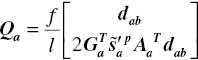
- Tyre vertical force
The tyre vertical force Qzj is given as:
(8.28)where z0j(t) is the road excitation; ktj is the tyre vertical stiffness; r0 is the tyre free radius; and zuj is the tyre vertical displacement. The filtered white noise described in Chapter 4 is selected as the road excitation in the time domain.
- Tyre lateral force and aligning moment
The Pacejka nonlinear tyre model is used to determine the dynamic forces of the tyre. The inputs of the tyre model include the tyre vertical force, tyre sideslip angle, and slip ratio; and the outputs include the lateral force Fy and aligning moment Mz. For the rigid multibody model, the front and rear sideslip angles are calculated as:
(8.29)
- Solution of the equations of motion
The equations of motion for the rigid multi-body expressed in equation (8.20) are a set of nonlinear differential-algebraic equations. Numerical methods to solve these equations include the direct method and the coordination separation method. Here, the direct method is used and programmed to obtain s and
 in equation (8.20). Then,
  is calculated by using equation (8.21) and the integral of
  is performed with respect to the generalized coordinates of the Euler parameters and the corresponding coordinates of the positions. Hence, the state variables, including the angular velocities and accelerations of the members, are obtained by solving equation (8.20). The flowchart showing how to solve these equations is shown in Figure 8.7.


Figure 8.6 Vehicle rigid multibody model. (1) Vehicle body. (2–5) Wheel member. (6) Steering column. (7) Tie rod.

Figure 8.7 Flow chart for solving the dynamic equations of motion.
8.2.2 Controller Design
A rule-based method is proposed to design the upper layer controller in order to coordinate the two lower layer controllers of the AFS and ASS. For the two lower layer controllers, two different working modes are designed for each controller according to the different control objectives under different driving conditions.
The upper layer controller monitors the driver’s intentions and the current vehicle state. Based on these input signals, the upper layer controller is designed to coordinate the interactions between the ASS and EPS in order to achieve the desired vehicle state. Thereafter, the control commands of switching to the appropriate working mode are generated by the upper layer controller and distributed to the two lower layer controllers respectively. Finally, each individual lower layer controllers executes their local control objectives to control the vehicle dynamics.
8.2.1.1 Design of the ASS Controller
Two working modes are considered in designing the ASS controller: (1) when the vehicle drives straight or the steering angle is relatively small, the control objective of the ASS is to improve the vehicle ride comfort; (2) when cornering, the control objective is to control or maintain the vehicle attitude to improve handling stability.
- Mode 1: Improving vehicle ride comfort
The ASS controller aims at improving vehicle ride comfort by controlling vehicle vertical acceleration and pitch angular acceleration. The increment PID control strategy is applied. The inputs to the PID controller include the tracking error of the vehicle pitch angular acceleration and the vertical acceleration, while the output is the ASS control force. The control law is obtained as:
where U(k) is the control force; e(k) is the tracking error; Kp, Kd, and Ki are the proportional, differential, integral coefficients of the PID controller, respectively. - Mode 2: Regulating vehicle position during cornering
In this working mode, the ASS controller regulates the roll and yaw motions during cornering. The appropriate control force of each ASS is obtained by applying the sliding mode variable structure control strategy developed in Section 8.2, and the switch function and control law are given in equation (8.17) and equation (8.18), respectively.
When regulating the roll motion, the control forces of the left-hand and right-hand side suspensions are regulated respectively. The input variables are selected as
 and
and  , and the output is the adjustment of the control force of the suspension
  (n =1, 2, 3, 4).
When regulating the yaw motion, the additional yaw moment is generated indirectly by adjusting the ASS control force, resulting in the regulation of the tyre forces. The inputs are defined as
 and
and  , where rd is the expected yaw rate given in equation (8.6). The output is the adjustment of the control force of the suspension
  (n = 1, 2, 3, 4).
In the rigid multibody dynamic model, the steering angle of the front wheel δf is derived according to the Euler parameter definition, by assuming that the tyre plane is vertical.
(8.32)
where e0fl and e0fr are the Euler parameters of the front-left and front-right wheels, respectively.
In addition, a weighting factor ε
 is defined to take into account the coupling effects of the roll and yaw motions, and ε is determined in real time according to the values of r and p. Hence, the corresponding suspension control force
  is defined as:(8.33)
8.2.1.2 Design of the EPS Controller
Similarly, two working modes are considered when designing the EPS controller: (1) when steering in steady-state, the objective of the EPS controller is to improve the ease of steering; (2) when the vehicle loses stability, e.g., oversteering, the assist torque must be reduced in order to weaken the driver’s ability to quickly change the steering angle of the front wheel, and hence increase the road feel.
- Mode 1: Improving steering ease
The increment PID control strategy is applied to the design of the EPS controller. The input to the PID controller is selected as the tracking error between the target current and the actual feedback current of the motor; while the output is the voltage of the motor. The target current is determined by the characteristic curve of the motor [5]. The control law has a similar expression as equation (8.30) and equation (8.31).
- Mode 2: Improving handling stability
The reduction of the assist torque is fulfilled by multiplying the steady-state target torque by a gain coefficient that is less than 1.
8.2.1.3 Design of an Upper Layer Coordinating Controller
A rule-based control method is adopted to design the upper layer coordinating controller. The structure of the multilayer control system is illustrated in Figure 8.8.

Figure 8.8 Block diagram of the multi-layer coordinating control system.
The control rule is developed as follows:
- Rule 1: When the vehicle drives straight or the steering angle is relatively small, the ASS controller works in mode 1 and the EPS system is idle.
- Rule 2: When cornering, the coordinating controller sends out the control command to the ASS controller to switch it to mode 2. Meanwhile, the coordinating controller recognizes the vehicle steering characteristics according to the tracking error er between the actual and expected yaw rate, combining the value of the steering angle of the front wheel. For example, when the vehicle steers to the left, er > 0 indicates the oversteering phenomenon. The coordinating controller sends out the control command to the EPS controller to work in mode 2. The gain coefficient values in mode 2 are then determined to reduce the extent of the oversteering. Otherwise, the EPS controller works in mode 1.
8.2.3 Simulation Investigation
A simulation study is performed in MATLAB to demonstrate the performance of the proposed multilayer coordinating control system. Two driving conditions are investigated, and the simulation results are illustrated in Figure 8.9. It is noted that the vehicle physical parameters presented in Table 7.5 are also used in the simulation. The following discussions are made:
- Driving condition 1: When the vehicle travels straight (or the steering angle is relatively small) at a speed of 20m/s, the upper layer controller works according to rule 1, i.e., the ASS works and EPS is idle. The vehicle ride comfort is the major control objective. It is observed clearly in Figure 8.9(a, b) that both the RMS and peak values of the vertical acceleration and pitch angular acceleration for the multilayer coordinating control system improve significantly compared with the passive suspension. Specifically, the RMS value of the vertical acceleration for the multilayer coordinating control system is reduced from 0.582m/s2 to 0.316m/s2, and the RMS value of the pitch angular acceleration from 0.673 rad/s2 to 0.496 rad/s2. The results indicate that the vehicle ride comfort is effectively enhanced.
- Driving condition 2: The vehicle travels at a speed of 10m/s and is subjected to a step steering input with amplitude of
 . The upper layer controller works according to rule 2. It is observed clearly in Figure 8.9(c) that the RMS value of the roll angular acceleration for the multilayer coordinating control system is reduced from 0.0389 rad/s2 to 0.0225 rad/s2, compared with the decentralized control system. As shown in Figure 8.9(d), both the peak value and settling time of the yaw rate for the multilayer coordinating control system are decreased greatly. In summary, the simulation results indicate that the multilayer coordinating controller is able to coordinate the interactions between the ASS and EPS. The application of multilayer coordinating controls effectively improves the overall vehicle performance including ride comfort and handling stability. In addition, the application of rigid multibody dynamics is successful in constructing and solving complex vehicle dynamic systems.

Figure 8.9 Simulation results. (a) Vehicle vertical acceleration. (b) Pitch angular acceleration. (c) Roll angular acceleration. (d) Yaw rate.
8.3 Multilayer Coordinating Control of an Active Suspension System (ASS) and Anti-lock Brake System (ABS)
This section studies the multilayer coordinating control of an active suspension system (ASS) and anti-lock brake system (ABS) to achieve the goal of function integration of the control systems[6,7]. The architecture of the proposed multilayer coordinating control system is shown in Figure 8.10. In the figure, ax is longitudinal deceleration and ![]() ; ΔTs and ΔTb represent the changes of the pitch torque and the braking torque, respectively; and uc is the wheel speed. The definitions of the other symbols in Figure 8.10 can be found in the previous section. The control system consists of three layers, i.e., coordinating layer, control layer, and target layer. The coordinating controller monitors the driver’s intentions and the current vehicle conditions including the pitch angle θ and longitudinal deceleration ax. Based on these input signals, the coordinating controller computes the desired vehicle motions in order to achieve an optimal overall performance criterion. Thereafter, the coordinating controller generates the control commands ΔTs and ΔTb to the two controllers, i.e., the ASS and the ABS, respectively. The ASS and the ABS in turn execute their local control objectives to apply (increase, decrease, or hold) the pitch torque Ts and the braking torque Tb, respectively.
; ΔTs and ΔTb represent the changes of the pitch torque and the braking torque, respectively; and uc is the wheel speed. The definitions of the other symbols in Figure 8.10 can be found in the previous section. The control system consists of three layers, i.e., coordinating layer, control layer, and target layer. The coordinating controller monitors the driver’s intentions and the current vehicle conditions including the pitch angle θ and longitudinal deceleration ax. Based on these input signals, the coordinating controller computes the desired vehicle motions in order to achieve an optimal overall performance criterion. Thereafter, the coordinating controller generates the control commands ΔTs and ΔTb to the two controllers, i.e., the ASS and the ABS, respectively. The ASS and the ABS in turn execute their local control objectives to apply (increase, decrease, or hold) the pitch torque Ts and the braking torque Tb, respectively.

Figure 8.10 Block diagram of the multilayer coordinating control system.
8.3.1 Coordinating Controller Design
It is known that interactions exist between the suspension system and brake system, especially when the brakes are applied. When the brakes are applied, the dynamic loads of the front wheel and rear wheel can be calculated by equation (8.34), based on the half vehicle model shown in Figure 8.11.
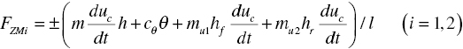
where cθ is pitch angular stiffness and ![]() ; hf and hr are the height of the C.G. for front and rear unsprung mass, respectively; h is the height of the C.G. of the vehicle; ks1 and ks2 are the stiffness of front suspension and rear suspension, respectively; and l is the wheelbase. A simple rule-based control strategy for the coordinating controller is designed as follows by using the two vehicle states, i.e., the pitch angle θ and longitudinal deceleration ax.
; hf and hr are the height of the C.G. for front and rear unsprung mass, respectively; h is the height of the C.G. of the vehicle; ks1 and ks2 are the stiffness of front suspension and rear suspension, respectively; and l is the wheelbase. A simple rule-based control strategy for the coordinating controller is designed as follows by using the two vehicle states, i.e., the pitch angle θ and longitudinal deceleration ax.

Figure 8.11 Half vehicle model.
- If
 , the coordinating controller monitors the vehicle states and does not generate control commands. In this case, the ABS is not applied, and only the EPS system executes its local control objective.
 - If
 , the coordinating controller coordinates the ASS system and the ABS in order to achieve an optimal overall performance criteria. Based on the pitch angle θ and longitudinal deceleration ax, the coordinating controller generates the control commands ΔTs and ΔTb to the two controllers, i.e., the ASS and the ABS, respectively. The ASS and the ABS in turn execute their local control objectives to apply the pitch torque Ts and the braking torque Tb, respectively.
Where a0 is the logic threshold of the deceleration; θ0 is the logic threshold of the pitch angle. It should be noted that these parameters have negative values. The pitch torque Ts and the braking torque Tb1 for front wheel and Tb2 for rear wheel are calculated as:


The proposed rule-based control strategy shows that only the deceleration and pitch angle exceed their thresholds, the coordinating controller generates the control commands to the ASS and ABS. Otherwise, the coordinating controller acts as a state monitor.
8.3.2 Simulation Investigation
A simulation study is performed to demonstrate the performance of the proposed multilayer coordinating control system. We assume that the vehicle travels at a constant speed uc = 20m/s, and the logic thresholds are selected as: ![]() , and
, and ![]() . The simulation results are shown in Figure 8.12(a–f). For comparison, the simulation for the decentralized control is also performed. In this case, we simply eliminate the upper layer controller. In addition, a quantitative analysis of the simulation result is also performed. The following discussions are made from the simulation results:
. The simulation results are shown in Figure 8.12(a–f). For comparison, the simulation for the decentralized control is also performed. In this case, we simply eliminate the upper layer controller. In addition, a quantitative analysis of the simulation result is also performed. The following discussions are made from the simulation results:

Figure 8.12 Simulation results. (a) Vertical acceleration of the sprung mass. (b) Pitch angle. (c) Longitudinal deceleration. (d) Brake distance. (e) Slip of the front wheel. (f) Slip of the rear wheel.
First, it is observed in Figure 8.12(a) that the peak values of the vertical acceleration of the sprung mass for the multilayer coordinating control is reduced compared to that of the decentralized control. Moreover, the R.M.S. (Root-Mean-Square) value of the performance index for the multilayer coordinating control shown in Table 8.1 is reduced greatly by 24.05%. A similar pattern can be observed for the performance index of the pitch angle. The results indicate that the ride comfort of the vehicle is improved significantly when the multilayer coordinating control is applied.
Table 8.1 Comparison of the R.M.S. values of the responses of the multilayer coordinating control and decentralized control.
| Performance index | Decentralized control | Multilayer coordinating control | Improvement |
| Vertical acceleration of sprung mass (m/s2) | 0.2320 | 0.1762 | 24.05% |
| Pitch angle (rad) | 0.0635 | 0.0526 | 17.17% |
| Longitudinal deceleration(m/s2) | 7.9714 | 8.1498 | 2.24% |
| Max. brake distance(m) | 24.306 | 23.734 | 0.572 |
In addition, it is shown in Figure 8.12(c) and (d) that both the longitudinal deceleration and the brake distance are improved slightly for the multilayer coordinating control compared to those of the decentralized control.
Finally, it is noted in Figure 8.12(e) that there is not much difference on the slip of the front wheel for the two control systems. However, the slip of the rear wheel for the multilayer coordinating control, as shown in Figure 8.12(f), is reduced clearly compared to that of the decentralized control. The results indicate that the brake swerve can be avoided, and hence the lateral stability is improved.
In summary, the multilayer coordinating controller is able to coordinate the interactions between the ASS and ABS. The application of the multilayer coordinating control improves the overall vehicle performance under critical driving conditions: the vehicle ride comfort is improved and the lateral stability is improved, and the braking performance is ensured.
8.4 Multilayer Coordinating Control of the Electric Power Steering System (EPS) and Anti-lock Brake System (ABS)
This section studies the multilayer coordinating control of an electric power steering system (EPS) and anti-lock brake system (ABS) to achieve the goal of function integration of the control systems[8,9]. Similar to Section 8.4, the architecture of the proposed multilayer coordinating control system is shown in Figure 8.13. Here, ΔTm and ΔTb represent the changes of the assist torque and the braking torque, respectively; and uc is the wheel speed. The definitions of the other symbols Figure 8.13 can be found in the previous section. The control system consists of three layers: coordinating layer, control layer, and target layer. The coordinating controller monitors the driver’s intentions and the current vehicle conditions including the torque applied on the steering wheel Tc, the vehicle speed uc, the slip λ, and the yaw rate γ. Based on these input signals, the coordinating controller computes the desired vehicle motions in order to achieve an optimal overall performance criterion. Thereafter, the coordinating controller generates the control commands ΔTm and ΔTb to the two controllers, i.e., the EPS system and the ABS, respectively. The EPS system and the ABS in turn execute their local control objectives to apply (increase, decrease, or hold) the assist torque Tm and the braking torque Tb, respectively.

Figure 8.13 Block diagram of the multilayer coordinating control system.
8.4.1 Interactions between the EPS System and ABS
To design the coordinating controller, we must first investigate the interactions between the EPS system and the ABS. An adhesion-slip curve of a tyre is used to reveal the interactions. Figure 8.14 illustrates the relationship between the slip and the lateral friction coefficient, and the relationship between the slip and the longitudinal friction coefficient.
Figure 8.14 Relationships of the slip and the friction coefficients (on a road surface with high adhesion).
Figure 8.14 shows that when the slip is less than 0.05, the lateral friction coefficient is relatively large, while the longitudinal friction coefficient is relatively small. Therefore, the vehicle is able to achieve a good lateral stability but a bad braking performance. When the slip is in the range between 0.1 and 0.3, the lateral friction coefficient drops dramatically while the longitudinal friction coefficient stays at a relatively large value. Therefore, the vehicle could have a good braking performance but a bad lateral stability. However, the performance conflicts between the steering system and the braking system have not been taken into account when designing the EPS system and the ABS separately. Therefore, it is necessary to coordinate the conflicts between the two control systems in order to obtain an optimal overall performance. The coordinating controller is designed as follows.
8.4.2 Coordinating Controller Design
A simple control strategy for the coordinating controller is designed as follows.
Three performance indices are considered in designing the coordinating controller, including the driver’s steering torque Tc, the slip λ for both the front wheel and rear wheel, and the yaw rate γ. The overall performance index J is defined as:

where J1, J2 and J3 are the variances of the driver’s steering torque Tc; the slip λ, and the yaw rate γ, respectively; W1, W2 and W3 are the weighting parameters. The following values are assigned to these weighting parameters, considering the relatively higher importance of the braking performance: W1 = 0.2, W2 = 0.5, and ![]() . For the first two indices, the driver’s steering torque Tc and the slip λ, three cases are considered:
. For the first two indices, the driver’s steering torque Tc and the slip λ, three cases are considered:
- If the vehicle speed is less than 20km/h, the coordinating controller does not generate any control commands. In this case, the ABS is not applied and only the EPS system executes its local control objective.
- If the vehicle speed is at the range of 20–40km/h, the coordinating controller coordinates the EPS system and the ABS to minimize the overall vehicle performance index defined in equation (8.38). In this case, the coordinating controller sends the control command of actuation to the EPS to adjust the assist torque according to the variation of the measured driver’s steering torque. In the meantime, the coordinating controller generates the control command of actuation according to the measured wheel angular acceleration and the slip. The ABS then adjusts the brake pressure of the wheel cylinders to guarantee the brake safety and the handling stability.
- If the vehicle speed is more than 40km/h, the coordinating controller does not generate any control commands. In this case, the EPS system is not applied, and only the ABS executes its local control objective.
The above control strategy is fulfilled through a decision-making controller. The main function of the decision-making controller is to monitor the driving conditions of the vehicle, and then decide whether or not the EPS system and ABS are applied. If both are applied, the decision-making controller coordinates the interactions between the two controllers.
For the third index, the yaw rate γ, a PID controller is designed to make the vehicle track the reference yaw rate. As shown in Figure 8.15, the reference yaw rate γd is obtained from the 2-DOF vehicle reference model derived in equation (8.6) since the 2-DOF reference model reflects the desired relationship between the driver’s steering input and the vehicle yaw rate. The block diagram of the PID controller is shown in Figure 8.15.

Figure 8.15 Block diagram of the PID controller.
In addition, it is noted that the controllers for the EPS system and ABS are designed in the same way as those in the previous chapter.
8.4.3 Simulation Investigation
A simulation study is performed to demonstrate the performance of the proposed multilayer coordinating control system. We assume that the vehicle travels at a constant speed of uc = 36 km/h, and is subjected to steering input from the steering wheel. In the meantime, an emergency brake is applied. The steering input is set as a step signal with an amplitude of 180°. After tuning the parameter setting for the coordinating PID controller, we select P = 86, I = 2, and D = 0.01 for the upper layer PID controller, and the optimal slip ![]() for the ABS.
for the ABS.
The simulation results for the three performance indices are shown in Figure 8.16(a)–(d). For comparison, the simulation for the decentralized control is also performed. In this case, we simply eliminate the upper layer controller. The following discussion is made from the simulation results.


Figure 8.16 Simulation results. (a) Yaw rate. (b) Driver’s steering torque. (c) Slip for the front wheel. (d) Slip for the rear wheel. (e) Brake distance.
First, it is observed that the yaw rate for the multilayer control, as shown in Figure 8.16(a), follows the desired yaw rate much better than that for the decentralized control. Moreover, it is also reduced more quickly than that for the decentralized control. The results indicate that the vehicle lateral stability is well controlled when the multilayer coordinating control is applied. Moreover, the driver’s steering torque for the multilayer coordinating control, as shown in Figure 8.16(b), is kept almost the same as that for the decentralized control. The results indicate that the steering agility is ensured when the multilayer coordinating control is applied. Finally, there is not much difference in wheel slip between the multilayer coordinating control and decentralized control, as can be seen in Figure 8.16(c) and (d). The results indicate that, inboth cases, the slip can be kept around the optimal value.
In addition, it is interesting to investigate the braking performance for both cases. The brake distances for both cases are shown in Figure 8.16(e). We can see from the figure that the brake distance for the multilayer coordinating control is slightly longer than that for the decentralized control. The reason for the small loss on the braking performance is that the steering direction is one of the factors when adjusting the brake pressure of the diagonal brake wheel cylinders under the simultaneous steering and braking driving conditions. However, the loss on the brake distance for the multilayer coordinating control in this investigation is too small to be taken into account.
In summary, the multilayer coordinating controller is able to coordinate the interactions between the EPS system and ABS. The application of the multilayer coordinating control improves the overall vehicle performance under the critical driving condition: the vehicle lateral stability is improved, and the steering agility and the braking performance are ensured.
8.5 Multi-layer Coordinating Control of the Active Suspension System (ASS) and Vehicle Stability Control (VSC) System
8.5.1 System Model
In this section, the 7-DOF nonlinear vehicle dynamic model, developed in the previous section, is used to calculate the vehicle dynamics of the system. The Pacejka nonlinear tyre model is used to determine the dynamic forces of each tyre. Again, the linear 2-DOF reference model is used for designing the controllers and calculating the desired response to the driver’s steering input. A filtered white noise signal is selected as the road excitation to the vehicle.
8.5.2 Multilayer Coordinating Controller Design
The architecture of the proposed multilayer coordinating control system is shown in Figure 8.17 [2,10]. The upper layer controller monitors the driver’s intentions and the current vehicle states including the vehicle speed uc, the steering angle of the front wheel δf, the sideslip angle β, the yaw rate r, and the lateral acceleration ay. Based on these input signals, the upper layer controller computes the corrective yaw moment Mzc in order to track the desired vehicle motions. Thereafter, the upper layer controller generates the distributed torques MVSC and MASS to the two lower layer controllers, i.e., the VSC and the ASS, respectively, according to a rule-based control strategy. Moreover, the distributed torques MVSC and MASS are converted into the corresponding control commands for the two individual lower layer controllers. Finally, the VSC and the ASS execute respectively their local objectives to control the vehicle dynamics. The upper layer controller and the two lower layer controllers are designed as follows.

Figure 8.17 Block diagram of the multilayer coordinating control system.
(Adapted from: Integrated Control of Active Suspension System and Electronic Stability Program Using Hierarchical Control Strategy: Theory and Experiment, by H. S. Xiao, W. W. Chen, H. H. Zhou, J. W. Zu. Reproduced with permission of the Taylor & Francis Group)
8.5.2.1 Upper Layer Controller Design
It is known that both the VSC and the ASS are able to develop corrective yaw moments (either directly or indirectly). To coordinate the interactions between the ASS and the VSC, a simple rule-based control strategy is proposed to design the upper layer controller. The aim of the proposed control rule is to distribute the corrective yaw moment appropriately between the two lower layer controllers. The control rule is described as follows.
First, the corrective yaw moment Mzc is calculated by using the 2-DOF vehicle reference model based on the measured and estimated vehicle input signals.
Second, the braking/traction torque Md and the pitch torque Mp are computed by using the following equations:

where equation (8.39) is derived by considering the dynamics of one of the front wheels. It should be noted that, although a front-wheel-drive vehicle is assumed, the main conclusions of this study can be easily extended to vehicles with other driveline configurations. In general, the brake torque at each wheel is a function of the brake pressure pw at that wheel, and cp is an equivalent braking coefficient of the braking system, which is determined by using the equation ![]() . The number “0.5” shows that the corrective yaw moment is evenly shared by the two front wheels.
. The number “0.5” shows that the corrective yaw moment is evenly shared by the two front wheels.
Finally, the distributed torques MESP and MASS are generated by using a linear combination of the braking/traction torque Md and the pitch torque Mp, which is given as:

where n1 and n2 are the weighting coefficients, and ![]() ,
, ![]() . Therefore, by tuning the weighting coefficients n1 and n2, the upper layer controller is able to coordinate with the two lower layer controllers and determine to what extent these are to be controlled.
. Therefore, by tuning the weighting coefficients n1 and n2, the upper layer controller is able to coordinate with the two lower layer controllers and determine to what extent these are to be controlled.
8.5.2.2 Lower Layer Controller Design
8.5.2.2.1 ASS controller design
The LQG control method is used to control the active suspension system. The state variables are defined as ![]() ; and the output variables are chosen as [
; and the output variables are chosen as [![]() . Therefore, the state equation and the output equation can be written as:
. Therefore, the state equation and the output equation can be written as:

where U = [U1 U2]T is the control input vector, and U1 = [f1 f2 f3 f4]T is the control force vector, U2 = [zg1 zg2 zg3 zg4]T is the road excitation vector. The multiple vehicle performance indices are considered to evaluate the vehicle handling stability, ride comfort, and safety. These performance indices can be measured by the following physical terms: vertical displacement of each wheel zu1, zu2, zu3, zu4; the suspension dynamic deflections ![]() ,
, ![]() ,
, ![]() ,
, ![]() ; the vertical acceleration of the sprung mass
; the vertical acceleration of the sprung mass ![]() ; the pitch angular acceleration
; the pitch angular acceleration ![]() ; the roll angular acceleration
; the roll angular acceleration ![]() ; and the control forces of the active suspension f1, f2, f3, f4. Therefore, the combined performance index is defined as:
; and the control forces of the active suspension f1, f2, f3, f4. Therefore, the combined performance index is defined as:

where q1,…, q11, and r1,…, r4 are the weighting coefficients. The above equation can be rewritten as the following matrix form:

where Q, R, N are the weighting matrices.
The state feedback gain matrix K is derived using the optimal control method, and it is the solution of the following Riccati equation:
8.5.2.2.2 VSC controller design
In this study, an adaptive fuzzy logic (AFL) method is applied to the design of the VSC controller [2]. The fuzzy logic controller (FLC) has been identified as an attractive control method in vehicle dynamics. This method has advantages when the following situations are encountered: (1) there is no explicit mathematical model that describes how the control outputs functionally depend on the control inputs; (2) there are experts who are able to incorporate their knowledge into the control decision-making process. However, traditional FLC with a fixed parameter setting cannot adapt to changes in the vehicle operating conditions or in the environment. Therefore, an adaptive mechanism must be introduced to adjust the controller parameters in order to achieve satisfactory vehicle performance in a wide range of changing conditions.
As shown in Figure 8.18, the AFL controller consists of a FLC and an adaptive mechanism. To design the AFL controller, the yaw rate and the sideslip angle of the vehicle are selected as the control objectives. The yaw rate can be measured by a gyroscope, but the sideslip angle cannot be measured directly and thus has to be estimated by an observer. The observer is designed by using the 2-DOF vehicle reference model. The linearized state space equation of the 2-DOF vehicle reference model is derived as follows, with the assumptions of having a constant forward speed and a small sideslip angle.

where,
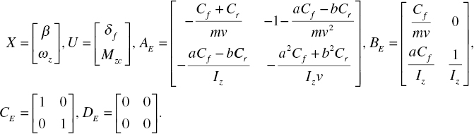

Figure 8.18 Block diagram of the adaptive fuzzy logic controller for the VSC.
The aim of the AFL is to track both the desired yaw rate and the desired sideslip angle. The desired yaw rate can be calculated using equation (8.6). As shown in Figure 8.19, the FLC has two input variables: the tracking error of the yaw rate e and the difference of the error de. They are defined as follows, at the k-th sampling time:

Figure 8.19 Comparison of responses for the step steering input maneuver. (a) Sideslip angle. (b) Yaw rate. (c) Lateral acceleration. (d) Vertical acceleration.
The output variable of the FLC is defined as the corrective yaw moment Mzc. To determine the fuzzy controller output for the given error and its difference, the decision matrix of the linguistic control rules is designed and presented in Table 8.2. These rules are determined based on expert knowledge and the large number of simulation results performed in the study. In designing the FLC, the scaling factors ke and kde have great effects on the performance of the controller. Therefore, the adaptive mechanism is applied to adjust the parameters in order to achieve a satisfactory control performance when there are changes in the vehicle operating conditions or in the environment. The adaptive law is given as in reference [2].


where ![]() .
.
Table 8.2 Fuzzy rule bases for VSC control.
|
de e |
PB | PM | PS | O | NS | NM | NB |
| PB | NB | NB | NB | NB | NM | O | O |
| PM | NB | NB | NB | NB | NM | O | O |
| PS | NM | NM | NM | NM | O | PS | PS |
| PO | NM | NM | NS | O | PS | PM | PM |
| NO | NM | NM | NS | O | PS | PM | PM |
| NS | NS | NS | O | PM | PM | PM | PM |
| NM | O | O | PM | PB | PB | PB | PB |
| NB | O | O | PM | PB | PB | PB | PB |
8.5.3 Simulation Investigation
In order to evaluate the performance of the developed multilayer coordinating control system, a simulation investigation is performed. We assume that the vehicle travels at a constant speed of uc = 90 km/h. Two driving conditions are performed: (1) step steering input, and (2) double lane change. For the first case, the vehicle is subjected to a steering input from the steering wheel and the steering input is set as a step signal with an amplitude of 120°. The road excitation is assumed to be independent for the four wheels.
After tuning the parameter setting for the multilayer coordinating control system, we select the set of weighting parameters for the ASS: ![]() ,
, ![]() ,
, ![]() ,
, ![]() ,
, ![]() , and
, and ![]() . Moreover, the weighting parameters for the upper layer controller are selected as:
. Moreover, the weighting parameters for the upper layer controller are selected as: ![]() and
and ![]() .
.
The simulation results for the multiple performance indices are shown in Figure 8.19 and Figure 8.20 (for brevity, only some representative performance indices are presented here). For comparisons, the simulation investigation for the decentralized control is also performed. In the case, we simply eliminate the upper layer controller. The following discussion is made:

Figure 8.20 Comparison of responses for the double lane change maneuver. (a) Sideslip angle. (b) Yaw rate. (c) Lateral acceleration. (d) Vertical acceleration.
- For the maneuver of step steering input, it can be seen that the peak value of the sideslip angle for the multilayer coordinating control, as shown in Figure 8.19(a), is reduced by 11.6% compared to that of the decentralized control. Moreover, the sideslip angle for the multilayer coordinating control is quickly damped and thus has less oscillation than that of the decentralized control. Similar patterns can be observed for the yaw rate and the lateral acceleration. The results indicate that the vehicle lateral stability is improved by the proposed multilayer coordinating control system compared to with the decentralized control system. In addition, the vertical acceleration of the spring mass, which is one of the ride comfort indices, is presented in Figure 8.19(d). It can be observed that the peak value of this performance index is decreased by 13.8% for the multilayer coordinating control compared to that of the decentralized control.
- For the double lane change maneuver, it is observed that the peak value of the sideslip angle for the multilayer coordinating control is reduced by 15.3% compared to that of the decentralized control, as shown in Figure 8.20(a). Moreover, for the peak value of the yaw rate shown in Figure 8.20(b), the percentage of decrease is 7.9%. However, as shown in Figure 8.20(c), there is no significant difference on the lateral acceleration between the two control cases. However, for the vertical acceleration of the spring mass shown in Figure 8.20(d), it can be clearly seen that the peak value of this performance index for the multilayer coordinating control is reduced significantly by 30.5% compared to that of the decentralized control. In addition, a quantitative analysis of the vertical acceleration shows that the R.M.S. (Root-Mean-Square) value of the vertical acceleration for the multi-layer coordinating control is reduced by 21.9% compared to that of the decentralized control.
In summary, the application of the multilayer coordinating control system improves the overall vehicle performance including the ride comfort and the lateral stability under critical driving conditions. The results show that the multilayer coordinating control system is able to coordinate the interactions between the ASS and the VSC and thus expand the functionalities of the two individual control systems.
8.6 Multilayer Coordinating Control of an Active Four-wheel Steering System (4WS) and Direct Yaw Moment Control System (DYC)
8.6.1 Introduction
As discussed in Chapter 5, the work principle of four-wheel steering (4WS) control is to simultaneously steer the rear wheels according to a specified relationship with the steering angles of the front wheels. Therefore, vehicle handling stability is improved by adjusting the tyre lateral forces. In general, the control strategy of the 4WS is designed based on the assumption that the tyre lateral force is proportional to the tyre steering angle. The assumption is valid only when the lateral acceleration is relatively small. However, when the lateral acceleration increases, the relationship among the tyre forces in the three directions and the steering angle of the wheels become nonlinear. This driving condition leads to difficulties in designing an appropriate control law to maintain vehicle stability.
There are quite a few control methods applied to the design of the 4WS, including adaptive control, robust control, and neural network. Adaptive control is able to achieve a great control performance when the lateral acceleration is relatively small. However, with adaptive control it is difficult to identify the real-time vehicle response parameters since the required steering angle is very small when a large lateral acceleration is reached. Hence, it is difficult to design an adaptive control system and maintain system stability. The application of the robust control method to the 4WS controller design ultimately results in solving linear matrix inequalities. The nonlinear error resulting from the decrease of the tyre lateral stiffness cannot be tolerated, and hence leads to system instability. In practice, this problem occurs under critical driving conditions including lane change (or cornering) combined with acceleration or deceleration. To overcome these difficulties, a control method based on neural network theory was proposed. The neural network-based control method is able to solve successfully the nonlinear problem caused by large tyre sideslip, and also adapt to vehicle parameter variations by tuning online the neural network coefficients.
At present, the application of the direct yaw moment control (DYC) exploits the limitations of the 4WS control systems. The DYC is able to handle effectively the saturation of the tyre lateral force and hence improve the vehicle lateral stability. In general, the yaw rate is selected as the control objective to adjust the tyre longitudinal forces since the yaw rate is more convenient to measure compared with the sideslip angle. However, it is more effective to maintain the vehicle trajectory through regulating directly the lateral tyre forces and therefore adjusting the sideslip angle. Therefore, the integrated control is able to improve significantly the vehicle lateral stability by combining the regulations of both the tyre lateral forces and longitudinal forces.
As discussed in Chapter 7, the keys to designing the integrated control system of the 4WS and DYC include: (1) coordinating the interactions between the two systems, and (2) exploiting the potentials of each subsystems. In this chapter, the integrated control of the 4WS and DYC regulates both the sideslip angle and the yaw rate to enhance overall vehicle performance over a large range of the lateral acceleration[11,12].
8.6.2 Coordinating Control of DYC and 4WS
8.6.2.1 Design of a Coordinating Control System
In this section the upper layer coordinating controller and two subsystem controllers for the DYC and 4WS are designed separately. In designing the 4WS controller, the sideslip angle is selected as the control objective since the 4WS adjusts directly the steering angle of the rear wheels. To simplify the design of the 4WS controller, the improvement of the steering sensitivity and lateral displacement are not taken into account. In addition, this simplification also results in a model with fewer degrees of freedom. Moreover, the yaw rate is selected as the control objective in designing the DYC controller. As illustrated in Figure 8.21, the upper layer coordinating controller monitors the driver’s intentions and the current vehicle states. Based on these input signals, the upper layer controller is designed to coordinate the interactions between the 4WS and DYC in order to achieve the desired vehicle states. The expected adjustment of the tyre longitudinal forces and steering angles of the real wheels are calculated. Thereafter, the control commands are generated by the upper layer controller and distributed to the two lower layer controllers respectively. Finally, the individual lower layer controllers execute respectively their local control objectives to control the vehicle dynamics. A rule-based control method is proposed to design the upper layer controller, and it is described as follows.

Figure 8.21 Coordinating system control configuration of the DYC and 4WS.
The expected yaw rate rd is an important performance index for the DYC system, which is defined as[12]:

where μ is the road adhesion coefficient; uc is the vehicle speed; g is the gravitational acceleration; l is the wheel base; K is the vehicle stability factor; and δf is the steering angle of the front wheel. It is known from equation (8.51) that the road adhesion coefficient and vehicle speed are vital parameters to determine the expected yaw rate.
The control objective of the 4WS controller is to make the sideslip angle close to 0. Therefore, the feedback control law of the 4WS controller derived from the linear 2-DOF vehicle reference dynamic model is given as:
where ![]() ;
;  ; δf and δr are the steering angles of the front and rear wheels, respectively; r is vehicle actual yaw rate; m is the vehicle mass; a and b are the horizontal distance between the center of gravity of the vehicle and the front and rear axles, respectively; kF and kR are the cornering stiffness of the front and rear wheels, respectively. It is known from equation (8.52) that the vehicle speed and the yaw rate are important parameters to determine the control output of the 4WS controller.
It is clear from the above discussion that the yaw rate is the major parameter affecting both subsystems, and it is not only the control objective of the DYC system, but also the important parameters determining the control output of the 4WS controller. In addition, both the road adhesion coefficient and vehicle speed determine the control outputs of the two subsytems. Therefore, the control rules for designing the upper layer coordinating controller are based on three factors, i.e., the yaw rate r, the road adhesion coefficient μ, and the vehicle speed uc.
It is known that the 4WS system is designed to have a specified speed ua. When the vehicle speed is lower than ua, the front and rear wheels steer in the opposite direction to reduce the vehicle steering radius and also improve steerability at low speeds. When the vehicle speed is higher than ua, the front and rear wheels steer in the same direction at a relatively small angle range to improve the vehicle transient steering characteristics, and also reduce the roll angle to a certain extent. Therefore, the control rules of the upper layer controller are developed according to the above two working conditions of the 4WS system. The detailed control rules are described as follows.
- When the vehicle drives straight or the steering angle is relatively small, the upper layer controller performs a supervision function, and no control command is sent out. In the meantime the DYC and 4WS systems are idle.
- When cornering:
- if
 , the upper layer controller performs the supervision function, and no control command is sent out. In the meantime the DYC system is idle; and the 4WS performs its local control objective to improve steerability at low speeds.
 - if
 , two thresholds of the yaw rate
  and
and  are determined to coordinate the two subsystems in different work domains. The two thresholds of the yaw rate
  and
and  are both positive, and
  .
.
- if
If  , and
, and ![]() , the upper layer controller generates the control commands and distributes those to the two subsystem controllers. The DYC controller works together with the 4WS controller and improves the steering sensitivity of the 4WS system. In the meantime, the 4WS controller performs its local control objective to improve the vehicle stability.
, the upper layer controller generates the control commands and distributes those to the two subsystem controllers. The DYC controller works together with the 4WS controller and improves the steering sensitivity of the 4WS system. In the meantime, the 4WS controller performs its local control objective to improve the vehicle stability.
If  and
and ![]() , the upper layer controller generates the control commands and distributes those to the two subsystem controllers. The DYC controller works together with the 4WS controller to improve the steering sensitivity of the 4WS system. In the meantime, the 4WS controller performs its local control objective to improve the vehicle stability.
, the upper layer controller generates the control commands and distributes those to the two subsystem controllers. The DYC controller works together with the 4WS controller to improve the steering sensitivity of the 4WS system. In the meantime, the 4WS controller performs its local control objective to improve the vehicle stability.
If  and
and ![]() , the upper layer controller generates the control commands and distributes those to the two subsystem controllers. The DYC controller improves the vehicle stability and, in the meantime, the 4WS system is idle.
, the upper layer controller generates the control commands and distributes those to the two subsystem controllers. The DYC controller improves the vehicle stability and, in the meantime, the 4WS system is idle.
Else, the upper layer controller performs the supervision function, and no control command is sent out. In the meantime the DYC system is idle; and the 4WS performs its local control objective to improve the vehicle stability.
In conclusion, the function allocation of the upper layer controller is based on the above rules. The upper layer controller generates the control command of improving steering sensitivity of the 4WS and distributes it to the DYC system. The DYC system works together with the 4WS and tracks the expected steady-state yaw rate generated by the linear 2-DOF vehicle dynamic reference model. The work domains of the two subsystems are divided by the two thresholds of the yaw rate and the upper layer controller coordinates and performs the function allocation of the two subsystems.
8.6.2.2 Lower Level Controller Design
- DYC controller design
The PID control method is applied to the design of the DYC controller to regulate the braking forces of the wheels. The calculation process of the PID control law is shown in Figure 8.22.
For simplification, the coordination between the ABS and the DYC is based on the slip ratio control approach. A target slip ratio of 0.2 is selected. When the slip ratio reaches or exceeds the target value, the ABS sends out the signal to reduce the braking pressure of the hydraulic cylinder in the brake system. If the tyre slip ratio is less than the target value, the proposed PID-based DYC controller works in this area.
- 4WS controller design
The neural network theory is applied to the design of the 4WS controller. The neural network-based control method is able to overcome the nonlinear problem caused by large tyre sideslip, and in the meantime adapt to vehicle parameter variations through tuning online the neural network coefficients. The detailed development of the control method can be found in Section 5.4.

Figure 8.22 Flowchart of the PID control algorithm.
8.6.3 Simulation Investigation
To demonstrate the performance of the proposed multilayer coordinating control system, a simulation investigation is performed by combining ADAMS and MATLAB for the dynamic analysis and control of the integrated control system. In the simulation, the vehicle speed is set as 80 km/h, the road adhesion coefficient is selected as 0.8, and the steering input to the steering wheel is a sinusoidal signal. The simulation results are shown in Figure 8.23 and a quantitative analysis of the results is presented in Table 8.3. In the figures, 2WS denotes that only the front steering system is used, and 4WS represents that only the 4WS system is used; 4WS + DYC represents that the proposed multilayer coordinating control system is applied.


Figure 8.23 Comparison of responses. (a) Yaw rate. (b) Sideslip angle. (c) Steering angle of the rear wheel. (d) Braking signal on each wheel. (e) Lateral displacement. (f) Traveling trajectory.
Table 8.3 Comparison of the peak value of responses.
| Peak value of performance index | 2WS | 4WS | 4WS + DYC |
| Yaw rate (deg/s) | 20.55 | 18.03 | 20.51 |
| Sideslip angle (deg) | 1.21 | 0.52 | 0.63 |
| Lateral displacement (m) | 6.17 | 4.47 | 5.56 |
It is shown in Figure 8.23(a) and Table 8.3 that the peak value of the yaw rate reaches 20.51 deg/s for the 4WS+DYC integrated control system. The value is closer to 20.55 deg/s for the 2WS system than 18.03 deg/s for the 4WS system. The results indicate that the proposed multilayer coordinating control system is able to track the expected yaw rate, and the steering sensitivity of the 4WS is improved. In addition, the settling time of the yaw rate for the multilayer coordinating control system is also reduced, compared with those for the other two systems. A similar pattern can also be observed for the sideslip angle.
It can be further concluded from Figure 8.23(e and f) that the lateral diaplacement response and traveling trajectory of the multilayer coordinating control system are close to those of the 2WS system. The results indicate that the multilayer coordinating control system is able to regulate the vehicle motions more accurately. The margin of the tyre lateral force is enlarged and, hence, the anti-sideslip ability is improved. While for the 4WS system, the deviations of the lateral displacement and traveling trajectory for the 2WS are significant even though the anti-sideslip ability of the 4WS is better. Moreover, both the lateral displacement and traveling trajectory of the 2WS demonstrate the phenomenon of sideslip to a certain extent.
In summary, the proposed multilayer coordinating control system is able to maintain the advantages of the 2WS, and also overcome its disadvantages through the coordination and function allocation of the 4WS and DYC systems. As a result, the vehicle stability is enhanced significantly.
8.7 Multilayer Coordinating Control of Integrated Chassis Control Systems
8.7.1 Introduction
As studied earlier in this chapter, the multilayer coordinating control method was applied to the coordination and function allocation of different combinations of two subsystem controllers, including ASS, DYC, ABS, EPS, AFS, and 4WS. However, it is known that the modern vehicle may be simultaneously equipped with more subsystem controllers on the steering, braking/traction, and suspension systems. Therefore, it is interesting to investigate the multilayer coordinating control of the overall vehicle dynamics in the three directions –lateral, longitudinal, and vertical – in order to enhance the overall vehicle performance including handling stability, ride comfort, acceleration and braking performance[13]. This is the aim of this section.
8.7.2 Controller Design
The architecture of the integrated control of chassis systems is illustrated in Figure 8.24. As analyzed in Chapter 6, the coupling effects among the three subsystems of steering, braking, and suspension are also presented in the figure. Based on the architecture, the structure of the multilayer coordinating control system is developed in Figure 8.25. Similarly, the upper layer controller monitors the driver’s intentions and the current vehicle states. Based on these input signals, the upper layer controller is designed to coordinate the interactions amongst the three subsystems by identifying the driving conditions of the vehicle in order to achieve the desired vehicle states. Thereafter, the control commands are generated by the upper layer controller according to the developed control rules for a certain driving condition of the vehicle. Then, the control commands are distributed to the three lower layer controllers respectively. Finally, the individual lower layer controllers execute respectively their local control objectives to control the overall vehicle dynamics. The three low layer controllers and the upper layer coordinating controller are developed as follows. It is noted that the detailed development of the vehicle dynamic model can be found in reference[13].
Figure 8.24 Architecture of the integrated chassis control system.

Figure 8.25 Block diagram of the multilayer coordinating control system.
8.7.2.1 Design of a Lower Level Controller
As shown in Figure 8.26, the PID control method is applied to the design of the controller of the suspension system. The PID controller is developed to adapt to the different driving conditions of the vehicle. When the vehicle drives in a normal condition, i.e., no emergency braking or cornering (the steering angle of the front wheel is relatively large) is applied, the vertical acceleration ![]() of the i-th suspension is selected as the control input. It is assumed at the k-th sampling time, the controller output is U(k) and the corresponding vertical acceleration at that time is
of the i-th suspension is selected as the control input. It is assumed at the k-th sampling time, the controller output is U(k) and the corresponding vertical acceleration at that time is ![]() . The PID control law for the i-th suspension is given as:
. The PID control law for the i-th suspension is given as:
where Kpi, Kii, and Kdi (i = 1, 2, 3, 4) are the proportional, differential, and integral coefficients, respectively. When the vehicle drives in the condition of either using emergency brakes or cornering, the aim of the PID controller is to regulate the pitch or the roll motions, and only the proportional coefficient Kpi is tuned while the other two are kept the same. Specifically, if regulating the pitch motion, the control inputs to the PID controller include the pitch angular velocity ![]() and its difference
and its difference ![]() , and the outputs are the weighting parameters of the PID controller Kpi, Kii, and Kdi (the parameters of the two front suspensions 1, 2 and the two rear suspensions 3, 4 are tuned in pairs). If regulating the roll motion, the control inputs to the PID controller include the roll rate
, and the outputs are the weighting parameters of the PID controller Kpi, Kii, and Kdi (the parameters of the two front suspensions 1, 2 and the two rear suspensions 3, 4 are tuned in pairs). If regulating the roll motion, the control inputs to the PID controller include the roll rate ![]() and its difference
and its difference ![]() . The outputs are the weighting parameters of the PID controller Kpi, Kii, and Kdi (the parameters of the two left suspensions 1,3 and two right suspensions 2,4 are tuned in pairs). It is noted that the driving conditions are determined by the upper layer controller and also the three weighting parameters of the PID controller are assigned by the upper layer controller.
. The outputs are the weighting parameters of the PID controller Kpi, Kii, and Kdi (the parameters of the two left suspensions 1,3 and two right suspensions 2,4 are tuned in pairs). It is noted that the driving conditions are determined by the upper layer controller and also the three weighting parameters of the PID controller are assigned by the upper layer controller.

Figure 8.26 Block diagram of the suspension PID control system.
The sliding mode variable structure control method is applied to the design of the DYC controller. The structure of the DYC system is illustrated in Figure 8.27 and the detailed development of the controller can be found in Section 8.2.

Figure 8.27 Block diagram of the DYC system.
The slip ratio control is applied to the design of the ABS, and the work principle of the slip ratio control is presented in Figure 8.28. The detailed development of the ABS controller refers to Section 3.3.

Figure 8.28 ABS control principle.
8.7.2.2 Design of the Upper Layer Controller
A rule-based control method is proposed to design the upper layer controller to coordinate the interactions among the three subsystems by identifying the driving conditions of the vehicle. The driving conditions of the vehicle can be divided into four types: (1) normal condition, i.e., no emergency brakes or cornering are applied; (2) normal condition and then emergency brakes; (3) normal condition and then sudden cornering; and (4) braking in turn. The different driving conditions are identified by calculating the measured signals from the sensors, including the vehicle longitudinal speed uc, lateral speed vc, longitudinal acceleration ![]() , lateral acceleration
, lateral acceleration ![]() , pitch rate
, pitch rate ![]() , roll rate
, roll rate ![]() , and steering angle of the hand wheel. The control rules of the upper layer coordinating controller are designed as follows.
, and steering angle of the hand wheel. The control rules of the upper layer coordinating controller are designed as follows.
Driving condition 1: The upper layer controller generates the control commands and distributes those to the three subsystem controllers. Both the ABS and DYC system are idle. The weighting parameters for the PID controller of the ASS are assigned according to the normal driving condition developed in the above section. These weighting parameters are kept unchanged throughout driving condition 1.
Driving condition 2: In this case, ABS works according to the tyre slip ratio control method and while the DYC system is idle. The set of the weighting parameters for the ASS PID controller are assigned and adjusted according to the driving condition concerning the pitch motions. The specific adjustment strategy for the weighting parameters is shown as follows by assuming that the counter clockwise direction around the y-axis is positive.
- If
 and
and  , then
  , and
, and  ;
; - If
 and
and  , then
  , and
, and  ;
; - If
 and
and  , then
  , and
, and  ;
; - If
 and
and  , then
  and
and  ;
; - If
 and
and  , then
  , and
, and  ;
; - If
 and
and  , then
  , and
, and  ;
; - If
 and
and  , then
  , and
, and  ;
; - If
 and
and  , then
  , and
, and  ;
; - If
 and
and  , then
  , and
, and  .
.
In addition, the values of the two weighting parameters Kii and Kdi are adjusted according to the adjustment chart presented in Table 8.4.
Table 8.4 Adjustment chart of the weighting parameters of the PID controller when pitching.
| 1.00 | 0.80 | 1.12 | |
| 1.06 | 0.80 | 1.00 | |
| 3.18 | 3.00 | 3.14 | |
| 3.16 | 3.00 | 3.24 | |
In the rule, the parameters αi and σi are obtained by tuning using enormous numbers of simulations, and in practice those can be calibrated in vehicle road tests. The parameters in the driving condition 3 are obtained by the same way.
Driving condition 3: In this case, the ABS is idle, and the DYC system generates the appropriate additional yaw moment to track the expected yaw rate. The set of the weighting parameters for the ASS PID controller are assigned and adjusted according to the driving condition concerning the roll motion. The specific adjustment strategy for the weighting parameters is shown as follows assuming that the counter clockwise direction around x axis is positive.
- If
 and
and  , then
  , and
, and  ;
; - If
 and
and  , then
  , and
, and  ;
; - If
 and
and  , then
  , and
, and  ;
; - If
 and
and  , then
  , and
, and  ;
; - If
 and
and  , then
  , and
, and  ;
; - If
 and
and  , then
  , and
, and  ;
; - If
 and
and  , then
  , and
, and  ;
; - If
 and
and  , then
  , and
, and  ;
; - If
 and
and  , then
  , and
, and  .
.
In addition, the values of the other two weighting parameters Kii and Kdi are adjusted according to the adjustment chart presented in Table 8.5.
Table 8.5 Adjustment chart of the weighting parameters of the PID controller when rolling.
| 1.06 | 0.8 | 1.10 | |
| 1.16 | 0.8 | 1.04 | |
| 3.10 | 3.0 | 3.12 | |
| 3.18 | 3.0 | 3.10 | |
Driving condition 4: In this case, both the ABS and the DYC system execute their functions based on the inputs of the measured signals. The set of weighting parameters for the ASS PID controller are assigned and adjusted according to the driving condition concerning the coupled roll and pitch motions. The specific adjustment strategy for the weighting parameters is shown as follows.
A weighting factor ε is defined in order to take into account the coupling effect of the roll and pitch motions during this driving condition. If ![]() , and
, and ![]() , the coupling effect is identified, and the proportional weighting parameter of the i-th suspension is regulated as:
, the coupling effect is identified, and the proportional weighting parameter of the i-th suspension is regulated as:
where ε0 and γ0 are the thresholds of the pitch and roll angular accelerations respectively, and their values are adjusted through tuning by simulations; ![]() and
and ![]() are the proportional weighting parameters of the i-th suspension obtained from the parameter assignment defined in the above pitch and roll driving conditions, respectively; and the value of ε is adjusted in real time by considering the values of
are the proportional weighting parameters of the i-th suspension obtained from the parameter assignment defined in the above pitch and roll driving conditions, respectively; and the value of ε is adjusted in real time by considering the values of ![]() and
and ![]() .
.
Otherwise, if the coupling effect of the roll and pitch motions are not identified, the maximum value of the pitch and roll angular accelerations, i.e., ![]() , is considered to identify which driving condition the vehicle performs on and, hence, the ASS is adjusted accordingly based on the above rules. In addition, the integral and differential weighting parameters of the ASS controller are assigned as follows[2].
, is considered to identify which driving condition the vehicle performs on and, hence, the ASS is adjusted accordingly based on the above rules. In addition, the integral and differential weighting parameters of the ASS controller are assigned as follows[2].
- If
 and
and  , then Ki = 1.0, Kd = 3.16;
 - else Ki = 0.8, and Kd =3.0.
8.7.3 Simulation and Experiment Investigations
8.7.3.1 Simulation Investigation
To demonstrate the performance of the proposed multi-layer integrated control system, a simulation investigation is performed by considering the four different driving conditions. The vehicle speed is set to 70km/h, and the physical parameters used in the simulation can be found in Table 7.5. The following discussion is made on the simulation results.
Driving condition 1: In this normal driving condition, the vehicle ride comfort is the performance index of most concern. It is observed in Figure 8.29(a) that the vehicle vertical acceleration for the multilayer integrated control system is improved greatly compared with that of the passive suspension.

Figure 8.29 Comparison of responses for the four different driving conditions. (a) Vehicle vertical acceleration (normal driving). (b) Yaw rate (step steering). (c) Roll angular acceleration (step steering). (d) Braking distance comparison (emergency brakes). (e) Pitch angular acceleration (emergency brake). (f) Vertical acceleration (braking in turn). (g) Yaw rate (braking in turn). (h) Braking distance (braking in turn).
Driving condition 2: For the step steering input maneuver the vehicle lateral stability is the performance index of most concern. It is observed in Figure 8.29(b) that the yaw rate for the multilayer integrated control system is better at tracking the expected yaw rate compared with that of the standalone DYC. In addition, it is obvious in Figure 8.29(c) that the roll angular acceleration for the multilayer integrated control system is reduced compared with that of the passive suspension, and the standalone ASS.
Driving condition 3: For the emergency brake maneuver, it is shown in Figure 8.29(d) that the brake distance for the multilayer integrated control system is reduced compared with that of the standalone ABS. In addition, it is shown in Figure 8.29(e) that the pitch angular acceleration for the multilayer integrated control system is also reduced compared with that of the standalone ASS based on the ordinary PID control and the passive suspension.
Driving condition 4: For the braking in turn maneuver, it is observed in Figure 8.29 (f)–(h) that the RMS of the vehicle vertical acceleration for the multilayer integrated control system is reduced by 3.1% and 25.8%, compared with that of the standalone ASS based on the ordinary PID control and the passive suspension, respectively. Moreover, the peak value of the yaw rate for the multilayer integrated control system is also reduced compared with that of the standalone DYC system. However, the brake distance for the multilayer integrated control system is increased compared with the standalone ABS system because of the intervention of the DYC system.
In summary, the application of the proposed multilayer coordinating control system is able to improve the overall vehicle dynamics in the lateral, longitudinal, and vertical directions and, hence, enhance the overall vehicle performance including handling stability, ride comfort, and braking performance.
8.7.3.2 Experiment Investigation
To validate the effectiveness of the control strategy, a vehicle road test is conducted. The configuration of the experiment setting is shown in Figure 8.30. The upper layer controller monitors the driver’s intentions and the current vehicle states measured by the sensors, including the speed, the steering angle of the front wheel, the yaw rate, the vertical, lateral, and longitudinal accelerations, and the pitch and roll angular accelerations. Based on these input signals, the upper layer controller generates control commands according to the above rule-based control method in order to control the overall vehicle dynamics. Then the control commands are distributed to the three lower layer controllers respectively. Finally, the individual lower layer controllers execute respectively their local control objectives.

Figure 8.30 Configuration of the vehicle coordinating control test. (1) Upper layer controller. (2) Solenoid valve drive. (3) Suspension controller. (4) Test vehicle. (5) Steering wheel angle sensor. (6) Gyroscope. (7) Acceleration sensor. (8) Vehicle speed sensor. (9) Data acquisition. (10) PC. (11) Power source with constant current. (12) Magneto rheological damper.
The experiment is performed by considering four different driving conditions. The following discussion is made on the simulation results. For driving condition 1, i.e., the normal driving condition, the RMS value of the vehicle vertical acceleration for the multilayer integrated control system is reduced from 1.02m/s2 to 0.96m/s2 compared with the passive suspension. For the emergency brake maneuver, the pitch angular acceleration of the multilayer integrated control system is also reduced from 0.41 rad/s2 to 0.34 rad/s2 compared with the standalone ASS based on the ordinary PID control. For the step steering input maneuver, the RMS value of the roll angular acceleration for the multilayer integrated control system is reduced from 0.034 rad/s2 to 0.029 rad/s2 compared with the standalone ASS. For the braking in turn maneuver, the peak value of the yaw rate for the multilayer integrated control system is also greatly reduced compared with that for the standalone DYC system. However, the brake distance for the multilayer integrated control system is increased compared with the standalone ABS system because of the intervention of the DYC system. In summary, the experiment results demonstrate a good agreement with the simulation results. Therefore, the application of the proposed multilayer coordinating control system is effective in enhancing the overall vehicle performance including handling stability, ride comfort, and braking performance.
8.8 Multilayer Coordinating Control of Integrated Chassis Control Systems using Game Theory and Function Distribution Methods
Due to the large number of chassis subsystems, it is hard for simple control systems to guarantee the system’s overall optimal control performance. When using hierarchy structures, however, the function of each level is clarified, i.e., the subcontrol system local performance is guaranteed by lower level controllers. The overall optimal performance of integrated control systems is guaranteed by upper level controllers. However, the functions of the chassis subsystems are different, for instance, the suspension subsystem can improve vehicle ride comfort and handling stability, and the braking subsystem can enhance the vehicle safety. To improve the chassis control system optimal performance, the function of each subsystem needs to be considered. An upper level controller needs to be designed to coordinate each subsystem and reach the optimal state of the chassis system overall control performance[14].
8.8.1 Structure of the Chassis Control System
As discussed in the previous section, the control strategy of the upper layer controller is applied to coordinate the interactions of the three subsystem controllers, and then fulfill the function distributions of the three controllers in order to improve the overall vehicle dynamics. In this section, game theory is applied to coordinate the conflicts amongst the different performance indices in order to determine the appropriate overall performance indices. In addition, the fuzzy logic control method is applied to the real-time self-tuning of the weighting parameters of the outputs of the subsystems to reduce the tracking errors between the actual control objectives of the lower layer controllers and the expected control objectives of the upper layer controller. The structure of the proposed multilayer coordinating control system is illustrated in Figure 8.31.

Figure 8.31 Block diagram of the multilayer coordinating control system.
8.8.2 Design of the Suspension Subsystem Controller
The ![]() control method is applied to the design of the controller of the suspension system in order to suppress the input disturbances and hence ensure the stability and robustness of the close loop control system of the suspension. A nonlinear state equation of the suspension system is established as:
control method is applied to the design of the controller of the suspension system in order to suppress the input disturbances and hence ensure the stability and robustness of the close loop control system of the suspension. A nonlinear state equation of the suspension system is established as:
where ![]() is the state vector; W = [z01 z02 z03 z04]T is the disturbance vector; and U = [fc1 fc2 fc3 fc4]T is the control input vector. The nonlinear output equation of the suspension system is obtained as:
is the state vector; W = [z01 z02 z03 z04]T is the disturbance vector; and U = [fc1 fc2 fc3 fc4]T is the control input vector. The nonlinear output equation of the suspension system is obtained as:
where ![]() is the measured output vector;
is the measured output vector; ![]() is the controlled output vector; fc1 through fc4 are the suspension control forces; zs is the displacement at the vehicle center of gravity; zs1 through zs4 are the suspension displacements; zu1 through zu4 are the wheel displacements; and z01 through z04 are the road displacements. The aim of the
is the controlled output vector; fc1 through fc4 are the suspension control forces; zs is the displacement at the vehicle center of gravity; zs1 through zs4 are the suspension displacements; zu1 through zu4 are the wheel displacements; and z01 through z04 are the road displacements. The aim of the ![]() control of the nonlinear suspension system is to design a stable close loop controller to generate the control forces and hence make the
control of the nonlinear suspension system is to design a stable close loop controller to generate the control forces and hence make the ![]() norm of the transfer function Tzw of the disturbance input W and the controlled output Z reach the minimum, i.e., min
norm of the transfer function Tzw of the disturbance input W and the controlled output Z reach the minimum, i.e., min ![]() . Based on the dissipation theory, the control law U(Y) is obtained so that the constructed close loop control system of the suspension satisfies the inequality of the L2 gain as follows:
. Based on the dissipation theory, the control law U(Y) is obtained so that the constructed close loop control system of the suspension satisfies the inequality of the L2 gain as follows:

where ![]() . When
. When ![]() is a positive definite matrix, the necessary and sufficient condition that the system is a p dissipation is the existence of a smooth and differentiable semi-positive storage function V(X(t)) with
is a positive definite matrix, the necessary and sufficient condition that the system is a p dissipation is the existence of a smooth and differentiable semi-positive storage function V(X(t)) with ![]() , and HJI inequalities are satisfied.
, and HJI inequalities are satisfied.
where,


Therefore, solving the nonlinear ![]() control problem is to find the control law U and the corresponding storage function V(X) defined in the above HJI inequalities through the Taylor series expansion method.
control problem is to find the control law U and the corresponding storage function V(X) defined in the above HJI inequalities through the Taylor series expansion method.
8.8.3 Design of the Steering Subsystem Controller
The PID control method is applied to the design of the controller of the DYC system. The expected yaw rate rd is defined in equation (8.51). After tuning, the weighting parameters of the PID controller are selected as Kp = 0.2, Ki = 0.5, and Kd = 0.1.
8.8.4 Design of the Braking Subsystem Controller
The sliding mode variable structure control method is applied to the design of the ABS in order to maintain the slip ratio around the target value to improve the system’s braking performance. The tracking error between the actual vehicle slip ratio λ and the expected value λd is defined as e = λ – λd. The switch function of the sliding mode controller is selected as ![]() . Therefore, the control law is given as
. Therefore, the control law is given as ![]() , where c0, α, and γ are the positive constants. After tuning, a good control performance is reached when c0 = 0.68,
, where c0, α, and γ are the positive constants. After tuning, a good control performance is reached when c0 = 0.68, ![]() 0.36, and γ = 0.06.
0.36, and γ = 0.06.
8.8.5 Design of the Upper Layer Controller
Game theory is applied to the design of the optimal control strategy in order to coordinate the conflicts amongst the performance indices and therefore achieve a global optimal performance. The basic principle of the game theory-based control strategy is described as follows. The control objectives of each subsystem are considered as a player in the game. Then the game matrix is constructed by the reciprocal of each control objective. Therefore, the global optimal solution of the control objective game problem is obtained through using the cooperative game method.
The control objective of the suspension is selected as ![]() in order to suppress the disturbance input to the suspension system. Moreover, the control objective of the DYC system is selected as
in order to suppress the disturbance input to the suspension system. Moreover, the control objective of the DYC system is selected as ![]() in order to track effectively the expected yaw rate. In addition, the control objective of the ABS is selected as
in order to track effectively the expected yaw rate. In addition, the control objective of the ABS is selected as  to regulate the slip ratio around the optimal value and reach the shortest braking distance. Here, s is the actual distance, and s0 is the braking distance when the simple logic control is applied. The payoff values of the game for the subsystem control objectives are defined as
 ![]() ,
, ![]() , and
, and ![]() , where a1, a2, and a3 are the coefficients. By considering the different driving conditions, including the emergency brakes, step steering input, and braking in turn, the corresponding payoff combinations of the game are obtained respectively as (m1, m3), (m1, m2), (m1, m2, m3). Therefore, the global optimal solution of the game problem is obtained as
, where a1, a2, and a3 are the coefficients. By considering the different driving conditions, including the emergency brakes, step steering input, and braking in turn, the corresponding payoff combinations of the game are obtained respectively as (m1, m3), (m1, m2), (m1, m2, m3). Therefore, the global optimal solution of the game problem is obtained as ![]() ,
, ![]() , and
, and ![]() through the cooperative game of the different subsystems; and
through the cooperative game of the different subsystems; and ![]() ,
, ![]() ,
, ![]() are the expected control objectives of the corresponding subsystems.
are the expected control objectives of the corresponding subsystems.
In addition, the fuzzy logic control method is applied to the real-time self-tuning of the weighting parameters of the outputs of the subsystems to reduce the tracking errors between the actual control objectives of the lower layer controllers and the expected control objectives of the upper layer controller. The control outputs of the subsystems include the control forces of suspension fci (![]() ), the additional yaw moment generated by the DYC system ΔM, and the braking torques of the brake system Tbi. The detailed strategy of the function distribution is developed as follows.
), the additional yaw moment generated by the DYC system ΔM, and the braking torques of the brake system Tbi. The detailed strategy of the function distribution is developed as follows.
For the emergency brake maneuver, ABS works according to the slip ratio control method, while the DYC system is idle. In addition, there is a conflict on the function distribution between the ASS and ABS because of the pitch motion. To guarantee the overall optimal performance, the coefficients are selected as a1 = 0.8 and a3 = 1.5. Then, the global optimal solutions ![]() and
and ![]() are obtained through the cooperative game of the two subsystems. Therefore, the expected control objectives of the ASS and ABS, i.e.,
are obtained through the cooperative game of the two subsystems. Therefore, the expected control objectives of the ASS and ABS, i.e., ![]() and
and ![]() respectively, are used to regulate in real time the control outputs of the ASS and ABS.
respectively, are used to regulate in real time the control outputs of the ASS and ABS.
In addition, the fuzzy logic control method is applied to the real-time self-tuning of the weighting parameters of the outputs of the subsystems, and the fuzzy logic controller is developed as follows, assuming a counter-clockwise direction around the y-axis positive.
The input variables of the fuzzy logic controller are defined as ![]() ,
, ![]() ,
, ![]() (
(![]() ); the discourse domain is defined as
); the discourse domain is defined as ![]() ; and the fuzzy subset is defined as ei,eci = {NS, NM, NS, ZO, PS, PM, PB}. The elements in the subset represent large negative, medium negative, small negative, null, small positive, medium positive, and large positive, respectively. It is assumed that the input variables ei, eci (i = 1,2) and the output variable qi are subject to Gaussian distribution. It is noted that the value of i is determined by the number of controlled outputs. For instance, for the ASS, i = 1, 2, 3, 4, for the DYC system i = 1, and for the ABS i = 1, 2, 3, 4. Therefore, the membership degree of each fuzzy subset can be determined. Based on the value assignment table of each subset membership degree and the fuzzy control model of each parameter, the fuzzy matrix of the output variables qi is obtained by applying the compositional rule of inference; next, the corrected parameter is found and then it is substituted into the equation
; and the fuzzy subset is defined as ei,eci = {NS, NM, NS, ZO, PS, PM, PB}. The elements in the subset represent large negative, medium negative, small negative, null, small positive, medium positive, and large positive, respectively. It is assumed that the input variables ei, eci (i = 1,2) and the output variable qi are subject to Gaussian distribution. It is noted that the value of i is determined by the number of controlled outputs. For instance, for the ASS, i = 1, 2, 3, 4, for the DYC system i = 1, and for the ABS i = 1, 2, 3, 4. Therefore, the membership degree of each fuzzy subset can be determined. Based on the value assignment table of each subset membership degree and the fuzzy control model of each parameter, the fuzzy matrix of the output variables qi is obtained by applying the compositional rule of inference; next, the corrected parameter is found and then it is substituted into the equation ![]() , where 1 is the initial value of the weighting parameter. In summary, the self-tuning of the output variables qi is fulfilled through the calculation process shown in Figure 8.32. The fuzzy self-tuning rule bases of the output variables qi of the ASS are shown in Table 8.6. A good control performance of the ASS is achieved when the fuzzy factors are selected as ke1 = 10 and
, where 1 is the initial value of the weighting parameter. In summary, the self-tuning of the output variables qi is fulfilled through the calculation process shown in Figure 8.32. The fuzzy self-tuning rule bases of the output variables qi of the ASS are shown in Table 8.6. A good control performance of the ASS is achieved when the fuzzy factors are selected as ke1 = 10 and ![]() 0.3, and the defuzzification factors as
0.3, and the defuzzification factors as ![]() = 0.1,
= 0.1, ![]() 0.08.
0.08.

Figure 8.32 Flowchart of online fuzzy self-tuning.
Table 8.6 Rule bases of fuzzy self-tuning of the ASS outputs.
| ec e |
NB | NM | NS | ZO | PS | PM | PB |
| NB | PB | PB | PM | PM | PS | ZO | ZO |
| NM | PB | PB | PM | PS | PS | ZO | NS |
| NS | PM | PM | PM | PS | ZO | NS | NS |
| ZO | PM | PM | PS | ZO | NS | NM | NM |
| PS | PS | PS | ZO | NS | NS | NM | NM |
| PM | PS | ZO | NS | NM | NM | NM | NB |
| PB | ZO | ZO | NM | NM | NM | NB | NB |
For the step steering input maneuver, the ABS is idle, and there is a conflict on the function distribution between the ASS and DYC because of the roll motion. Similarly, to guarantee the overall optimal performance, the coefficients are selected as a1 = 0.9 and a2 = 1.2. Then the global optimal solutions ![]() and
and ![]() are obtained through the cooperative game of the two subsystems. Therefore, the expected control objectives of the ASS and DYC, i.e.,
are obtained through the cooperative game of the two subsystems. Therefore, the expected control objectives of the ASS and DYC, i.e., ![]() and
and ![]() respectively, are used to regulate in real time the control outputs of the ASS and DYC.
respectively, are used to regulate in real time the control outputs of the ASS and DYC.
For the braking in turn maneuver, the three subsystems perform the control functions according to the following rule. The expected slip ratio λd is regulated in real time by the upper layer controller. There are conflicts on the function distributions among the three subsystems because of the coupled pitch and roll motions. Similarly, to guarantee the overall optimal performance, the coefficients are selected as a1 = 0.79, a2 = 1.16, and a3 = 1.38. Then, the global optimal solutions ![]() ,
, ![]() and
and ![]() are obtained through the cooperative game of the two subsystems. Therefore, the expected control objectives of the three subsystems ASS, DYC, and ABS, i.e.,
are obtained through the cooperative game of the two subsystems. Therefore, the expected control objectives of the three subsystems ASS, DYC, and ABS, i.e., ![]() ,
, ![]() , and
, and ![]() respectively, are used to regulate in real time the control outputs of the three subsystems.
respectively, are used to regulate in real time the control outputs of the three subsystems.
8.8.6 Simulation Investigation
To demonstrate the performance of the proposed multilayer integrated control system, a simulation investigation is performed by considering the three different driving conditions. The vehicle speed is set to 70km/h and the physical parameters used in the simulation can be found in Table 7.5. The following discussions are made based on the simulation results shown in Figures 8.33–8.35.

Figure 8.33 Comparison of responses for the step steering input maneuver. (a) Yaw rate. (b) Roll angular acceleration.

Figure 8.34 Comparison of responses for the emergence brake maneuver. (a) Brake distance. (b) Pitch angular acceleration.

Figure 8.35 Comparison of responses for the braking in turn maneuver. (a) Vehicle vertical acceleration (b) Yaw rate. (c) Brake distance.
For the step steering input maneuver, it is observed in Figure 8.33(a) that the yaw rate for the multilayer integrated control system is better on tracking the expected yaw rate, compared with that of the decentralized control system (i.e., the three subsystems work independently). In addition, it is obvious in Figure 8.33(b) that the roll angular acceleration for the multilayer integrated control system is reduced significantly compared with that of the decentralized control system. The simulation results indicate that the proposed multilayer integrated control system is able to achieve a better handling stability and ride comfort than the decentralized control system.
For the emergency brakes maneuver, it is observed in Figure 8.34 that both the brake distance and the pitch angular acceleration for the multilayer integrated control system is reduced compared with that of the decentralized control system. The simulation results indicate that the proposed multilayer integrated control system is able to achieve a better braking performance and ride comfort than the decentralized control system.
For the braking in turn maneuver, it is observed in Figure 8.35(a) that the peak value and RMS of the vertical acceleration for the multilayer integrated control system is reduced compared with that of the decentralized control system. In addition, the settling time of the vertical acceleration for the multilayer integrated control system is also reduced. Moreover, as shown in Figure 8.35(b), the peak value of the yaw rate for the multilayer integrated control system is also reduced. However, the brake distance for the multilayer integrated control system is increased compared with that for the decentralized control system because of the intervention of the DYC system.
In summary, the application of the proposed multilayer coordinating control system is able to improve the overall vehicle dynamics in the three directions including lateral, longitudinal, and vertical and, hence, enhance the overall vehicle performance including handling stability, ride comfort, and braking performance.
References
- [1] Gordon T J, Howell M, Brandao F. Integrated control methodologies for road vehicles. Vehicle System Dynamics, 2003, 40(1–3), 157–190.
- [2] Xiao H S, Chen W W, Zhou H H, Zu J W. Integrated control of active suspension system and electronic stability program using hierarchical control strategy: Theory and experiment. Vehicle System Dynamics, 2011, 49(1/2), 381–397.
- [3] Zhu H, Chen W W. Active control of vehicle suspension and steering systems based on hierarchical control method. Transactions of the Chinese Society for Agricultural Machinery, 2008, 39(10), 1–6 (in Chinese).
- [4] Wang Q D, Qing W H, Chen W W. Integrated control of vehicle ASS and EPS based on Multi-degree of Freedom Model. Journal of System Simulation, 2009, 21(16), 5130–5137 (in Chinese).
- [5] Qing W H. Integrated Chassis Control using Multi-body Model. PhD Thesis, Hefei University of Technology, Hefei, China, 2010 (in Chinese).
- [6] Chu C B. Hierarchical Control of Chassis Systems. PhD Thesis, Hefei University of Technology, Hefei, China, 2008.
- [7] ChuC B, ChenW W. Hierarchical control of chassis systems. Journal of Mechanical Engineering, 2008, 44(2), 157–162 (in Chinese).
- [8] Chen W W, Chu C B. Hierarchical control of electrical power steering system and anti-lock brake system. Journal of Mechanical Engineering, 2009, 45(7), 188–193 (in Chinese).
- [9] ChenW W, Xiao H S, Chu C B, Zu J W. Hierarchical control of automotive electric power steering system and anti-lock brake system: Theory and experiment. International Journal of Vehicle Design, 2012, 59(1), 23–43.
- [10] Chen W W, Zhou H H, Liu X Y. Hierarchical control of ESP and ASS. Journal of Mechanical Engineering, 2009, 45(8), 190–196 (in Chinese).
- [11] Song Y. Vehicle Stability Control System and Four-wheel Steering System and its Integrated Control. PhD Thesis, Hefei University of Technology, Hefei, China, 2012 (in Chinese).
- [12] Song Y, Chen W W, Chen L Q. Simulation of vehicle stability control through combining ADAMS and MATLAB. Journal of Mechanical Engineering, 2011, 47(16), 86–92 (in Chinese).
- [13] Chen W W, Zhu H. Coordination control of vehicle handling stability and ride comfort based on state identification. Journal of Mechanical Engineering, 2011, 47(6), 121–129 (in Chinese).
- [14] Wang H B, Chen W W, Yang L Q, et al. Coordination control of vehicle chassis systems based on game theory and function distribution. Journal of Mechanical Engineering, 2012, 48(22), 105–112 (in Chinese).