
CHAPTER FIVE
N-Person Nonzero Sum Games and Games with a Continuum of Strategies
The race is not always to the swift nor the battle to the strong, but that’s the way to bet.
—Damon Runyon, More than Somewhat
5.1 The Basics
In previous chapters, the games all assumed that the players each had a finite or countable number of pure strategies they could use. A major generalization of this is to consider games in which the players have many more strategies. For example, in bidding games the amount of money a player could bid for an item tells us that the players can choose any strategy that is a positive real number. The dueling games we considered earlier are discrete versions of games of timing in which the time to act is the strategy. In this chapter, we consider some games of this type with N players and various strategy sets.
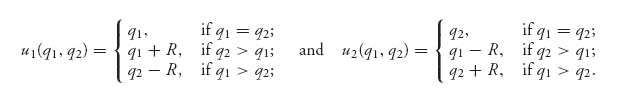
If there are N players in a game, we assume that each player has her or his own payoff function depending on her or his choice of strategy and the choices of the other players. Suppose that the strategies must take values in sets Qi, i = 1, …, N and the payoffs are real-valued functions:
![]()
Here is a formal definition of a pure Nash equilibrium point, keeping in mind that each player wants to maximize their own payoff.
Definition 5.1.1 A collection of strategies q* = (q1*, …, qn*) ![]() Q1 × · · · × QN is a pure Nash equilibrium for the game with payoff functions { ui(q1, …, qn)}, i = 1, …, N, if for each player i = 1, …, N, we have
Q1 × · · · × QN is a pure Nash equilibrium for the game with payoff functions { ui(q1, …, qn)}, i = 1, …, N, if for each player i = 1, …, N, we have
A short hand way to write this is ui(qi*, q−i*) ≥ ui (qi, q−i*) for allqi ![]() Qi, where q−i refers to all the players except the ith.
Qi, where q−i refers to all the players except the ith.
A Nash equilibrium consists of strategies that are all best responses to each other. The point is that no player can do better by deviating from a Nash point, assuming that no one else deviates. It doesn’t mean that a group of players couldn’t do better by playing something else.
Remarks 1. Note that if there are two players and u1 = −u2, then a point (q1*, q2*) is a Nash point if
![]()
But then
and putting these together we see that
![]()
This, of course, says that (q1*, q2*) is a saddle point of the two-person zero sum game. This would be a pure saddle point if the Q sets were pure strategies and a mixed saddle point if the Q sets were the set of mixed strategies.
2. In many cases, the problem of finding a Nash point can be reduced to a simple calculus problem. To do this we need to have the strategy sets Qi to be open intervals and the payoff functions to have at least two continuous derivatives because we are going to apply the second derivative test. The steps involved in determining (q1*, q2*, …, qn*) as a Nash equilibrium are the following:
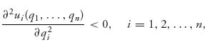
evaluated at q1*, …, qn*.
If these three points hold for (q1*, q2*, …, qn*), then it must be a Nash equilibrium. The last condition guarantees that the function is concave down in each variable when the other variables are fixed. This guarantees that the critical point (in that variable) is a maximum point. There are many problems where this is all we have to do to find a Nash equilibrium, but remember that this is a sufficient but not necessary set of conditions because many problems have Nash equilibria that do not satisfy any of the three conditions.
3. Carefully read the definition of Nash equilibrium. For the calculus approach we take the partial of ui with respect to qi, not the partial of each payoff function with respect to all variables. We are not trying to maximize each payoff function over all the variables, but each payoff function to each player as a function only of the variable they control, namely, qi. That is the difference between a Nash equilibrium and simply the old calculus problem of finding the maximum of a function over a set of variables.
Let’s start with a straightforward example.
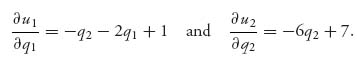
Example 5.1 We have a two-person game with pure strategy sets Q1 = Q2 = ![]() and payoff functions
and payoff functions

Then
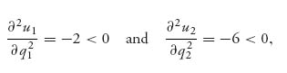
There is one and only one solution of these (so only one stationary point), and it is given by q1 = − ![]() , q2 =
, q2 = ![]() . Finally, we have
. Finally, we have
and so (q1, q2) = (− ![]() ,
, ![]() ) is indeed a Nash equilibrium.
) is indeed a Nash equilibrium.
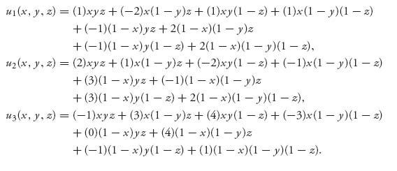
For a three-person example take
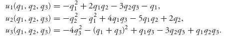
Taking the partials and finding the stationary point gives the unique solution q1* = ![]() , q2* =
, q2* = ![]() , and q3* =
, and q3* = ![]() . Since ∂2 u1/∂q12 = −2 < 0, ∂2 u2/∂ q22 = −2 < 0, and ∂2 u3/∂ q32 = −10 < 0, we know that our stationary point is a Nash equilibrium.
. Since ∂2 u1/∂q12 = −2 < 0, ∂2 u2/∂ q22 = −2 < 0, and ∂2 u3/∂ q32 = −10 < 0, we know that our stationary point is a Nash equilibrium.
This example has found a pure Nash equilibrium that exists because the payoff functions are concave in each variable separately. When that is not true we have to deal with mixed strategies that we will discuss below.
Best response strategies play a critical role in finding Nash equilibria. The definition for games with a continuum of strategies is given next.
Definition 5.1.2 Given payoff functions ui(q1, …, qn), a best response of player k, written qk = BRk (q1, …, qk−1, qk + 1, …, qn) is a value that satisfies
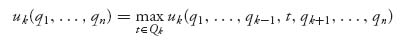
or uk(qk, q−k) = maxt ![]() Qk uk(t, q−k). In other words, qk provides the maximum payoff for player k, given the values of the other player’s qi′s.
Qk uk(t, q−k). In other words, qk provides the maximum payoff for player k, given the values of the other player’s qi′s.
In general, we say that qk = BRk (q−k) ![]() arg maxx uk(qk, q−k) 1 where we use the notation
arg maxx uk(qk, q−k) 1 where we use the notation
![]()
![]()
Example 5.2 This example will illustrate the use of best response strategies to calculate a Nash equilibrium.
Suppose players I and II have payoff functions
![]()
The variables must be nonnegative, x ≥ 0, y ≥ 0.
First, we find the best response functions for each player, namely, y(x) that satisfies u2(x, y(x)) = maxy u2 (x, y), and x(y) that satisfies u1 (x(y), y) = maxx u1 (x, y).
For our payoffs ![]() = 0
= 0 ![]() x(y) = 1 + y, and
x(y) = 1 + y, and ![]() = 0
= 0 ![]() y(x) =
y(x) = ![]() . This requires 4 ≥ x ≥ 0. The Nash equilibrium is where the best response curves cross, that is, where x(y) = y(x). For this example, we have x* = 2 and y* = 1. Taking the second partials show that these are indeed maxima of the respective payoff functions. Furthermore, u1 (2, 1) = 4 and u2 (2, 1) = 1.
. This requires 4 ≥ x ≥ 0. The Nash equilibrium is where the best response curves cross, that is, where x(y) = y(x). For this example, we have x* = 2 and y* = 1. Taking the second partials show that these are indeed maxima of the respective payoff functions. Furthermore, u1 (2, 1) = 4 and u2 (2, 1) = 1.
Knowing the best response functions allow us to consider what happens if the players choose sequentially instead of simultaneously.
Suppose that player I assumes that II will always use the best response function y(x) = ![]() . Why wouldn’t player I then choose x to maximize u1 (x, y (x)) = x (2 + 2(
. Why wouldn’t player I then choose x to maximize u1 (x, y (x)) = x (2 + 2(![]() ) − x)? This function has a maximum at x =
) − x)? This function has a maximum at x = ![]() and u1 (
and u1 (![]() , y(
, y(![]() )) =
)) = ![]() > 4. Thus, player I can do better if she knows that player II will use her best response function. Also, since y(
> 4. Thus, player I can do better if she knows that player II will use her best response function. Also, since y(![]() ) =
) = ![]() , u2 (
, u2 (![]() ,
, ![]() ) =
) = ![]() > 1, both players do better if they play in this manner. On the other hand, if player I uses x =
> 1, both players do better if they play in this manner. On the other hand, if player I uses x = ![]() and player II uses y = 1, then u1 (
and player II uses y = 1, then u1 (![]() , 1) =
, 1) = ![]() < 4 and u2 (
< 4 and u2 (![]() , 1) =
, 1) = ![]() > 1.
> 1.
Similarly, if player II chooses her point y to maximize u2(x(y), y), she will see that y = ![]() and then x(
and then x(![]() ) =
) = ![]() . Then u1 (
. Then u1 (![]() ,
, ![]() ) =
) = ![]() > 4 and u2 (
> 4 and u2 (![]() ,
, ![]() ) =
) = ![]() > 1. Only player II does better in this setup.
> 1. Only player II does better in this setup.
The conclusion is that both players prefer that player II commits to using her best response and that player I announces she will play x = ![]() .
.
It is not true that Nash equilibria can be found only for payoff functions that have derivatives but if there are no derivatives then we have to do a direct analysis. Here is an example.
Example 5.3 Do politicians pick a position on issues to maximize their votes2 Suppose that is exactly what they do (after all, there are plenty of real examples). Suppose that voter preferences on the issue are distributed from [0, 1] according to a continuous probability density function f(x) < 0 and ∫01 f(x); dx = 1. The density f(x) approximately represents the percentage of voters who have preference x ![]() [0, 1] over the issue. The midpoint x =
[0, 1] over the issue. The midpoint x = ![]() is taken to be middle of the road, while x values in [0,
is taken to be middle of the road, while x values in [0, ![]() ) are leftist, or liberal, and x values in (
) are leftist, or liberal, and x values in (![]() , 1] are rightist, or conservative. The question a politician might ask is “Given f, what position in [0, 1] should I take in order to maximize the votes that I get in an election against my opponent?” The opponent also asks the same question. We assume that voters will always vote for the candidate nearest to their own positions.
, 1] are rightist, or conservative. The question a politician might ask is “Given f, what position in [0, 1] should I take in order to maximize the votes that I get in an election against my opponent?” The opponent also asks the same question. We assume that voters will always vote for the candidate nearest to their own positions.
Let’s call the two candidates I and II, and let’s take the position of player I to be q1 ![]() [0, 1] and for player II, q2
[0, 1] and for player II, q2 ![]() [0, 1]. Let V be the random variable that is the position of a randomly chosen voter so that V has continuous density function f.
[0, 1]. Let V be the random variable that is the position of a randomly chosen voter so that V has continuous density function f.
The payoff functions for player I and II are given by
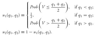
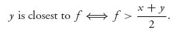
Here is the reasoning behind these payoffs. Suppose that q1 > q2, so that candidate I takes a position to the left of candidate II. The midpoint of
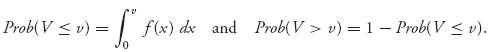
![]()
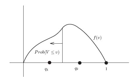
Now, the voters below q1 will certainly vote for candidate I because q2 is farther away. The voters above q2 will vote for candidate II. The voters with positions in the interval [q1, γ] are closer to q1 than to q2, and so they vote for candidate I. Consequently, candidate I receives the total percentage of votes Prob (V ≤ γ = (q1 + q2)/2) if q1 < q2. Similarly, if q2 < q1, candidate I receives the percentage of votes Prob (V > γ). Finally, if q1 = q2, there is no distinction between the candidates’ positions and they evenly split the vote. Recall from elementary probability theory (see Appendix B) that the probabilities for a given density are given by (see Figure 5.1):
This is a problem with a discontinuous payoff pair, and we cannot simply take derivatives and set them to zero to find the equilibrium. But we can take an educated guess as to what the equilibrium should be by the following reasoning. Suppose that I takes a position to the left of II, q1 < q2. Then she receives Prob(V ≤ γ) percent of the vote. Because this is the cumulative distribution function of V, we know that it increases as γ (which is the midpoint of q1 and q2) increases. Therefore, player I wants γ as large as possible. Once q1 increases past q2, then candidate II starts to gain because u1(q1, q2) = 1 − Prob (V ≤ γ) if q1 > q2. It seems that player I should not go further to the right than q2, but should equal q2. In addition, we should have
![]()
In probability theory, we know that this defines γ as the median of the random variable V. Therefore, the equilibrium γ should be the solution of
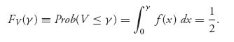
Because FV′(γ) = f(γ) > 0, FV(γ) is strictly increasing, and there can only be one such γ = γ* that solves the equation; that is, a random variable has only one median when the density is strictly positive.
On the basis of this reasoning, we now verify that
![]()
then
![]()
If this is the case, then ui(γ*, γ*) = ![]() for each candidate and both candidates split the vote.
for each candidate and both candidates split the vote.
How do we check this? We need to verify directly from the definition of equilibrium that
for every q1, q2 ![]() [0, 1]. If we assume q1 > γ*, then
[0, 1]. If we assume q1 > γ*, then

If, on the other hand, q1 < γ*, then

and we are done.
In the special case, V has a uniform distribution on [0, 1], so that Prob(V ≤ v) = v, 0 ≤ v ≤ 1, we have γ* = ![]() . In that case, each candidate should be in the center. That will also be true if voter positions follow a bell curve (or, more generally, is symmetric). It seems reasonable that in the United States if we account for all regions of the country, national candidates should be in the center. Naturally, that is where the winner usually is, but not always. For instance, when James Earl Carter was president, the country swung to the right, and so did γ*, with Ronald Reagan elected as president in 1980. Carter should have moved to the right.
. In that case, each candidate should be in the center. That will also be true if voter positions follow a bell curve (or, more generally, is symmetric). It seems reasonable that in the United States if we account for all regions of the country, national candidates should be in the center. Naturally, that is where the winner usually is, but not always. For instance, when James Earl Carter was president, the country swung to the right, and so did γ*, with Ronald Reagan elected as president in 1980. Carter should have moved to the right.
FIGURE 5.1 Area to the left of v is candidate I’s percentage of the vote.
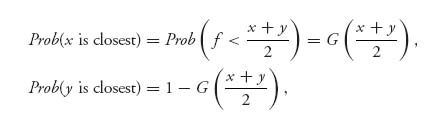
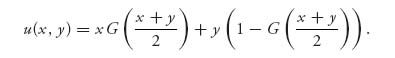
Example 5.4 Negotiation with Arbitration. A firm is negotiating with the union for a new contract on wages. As often happens (NBA vs. Player’s Union 2011), the negotiations have gone to an arbitrator in an effort to insert a neutral party to decide the issue. The offers are submitted to the arbitrator simultaneously by the firm and the union. Suppose the offers are x by the firm and y by the union and we may assume y > x, since if the firm offers at least what the union wants the problem goes away. The arbitrator has in mind a settlement he considers fair, say f and the offer submitted closest to f will be the one the arbitrator selects and will impose this as the settlement. The amount f is known only to the arbitrator but the firm and union guess that f is distributed according to some known cumulative probability distribution function G (x) = Prob (f ≤ x).
The parties know that the arbitrator will choose the closest offer to f and so each calculates the expected payoff
![]()
Of course, it must be true that x < f < y. By drawing a number line it is easy to see that
![]()
and
Thus,
and
This is a two-person zero sum game. The union is the maximizer and the firm is the minimizer. It is a calculus calculation to check that
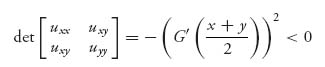
as long as G′(![]() ) ≠ 0. At any such point, if the first derivatives are zero there, the point must be a saddle point.
) ≠ 0. At any such point, if the first derivatives are zero there, the point must be a saddle point.
To find a saddle point, we calculate
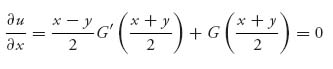
and
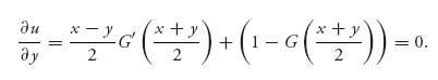
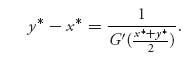
Solving for x*, y* we see that G (![]() ) =
) = ![]() . We interpret this to say that there are many possible offers that each of the two sides can make, but the saddle point must satisfy the requirement that the average of the two offers should be a median of the arbitrator’s distribution. Of course, neither player knows the other’s offer but they can calculate the median of G and then propose that offer. The average of the two offers will give the median. Since this is a saddle point, any deviation from that will not be optimal for the deviant player.
. We interpret this to say that there are many possible offers that each of the two sides can make, but the saddle point must satisfy the requirement that the average of the two offers should be a median of the arbitrator’s distribution. Of course, neither player knows the other’s offer but they can calculate the median of G and then propose that offer. The average of the two offers will give the median. Since this is a saddle point, any deviation from that will not be optimal for the deviant player.
Next, since G(![]() ) =
) = ![]() we may substitute this into either ux = 0 or uy = 0 to see that
we may substitute this into either ux = 0 or uy = 0 to see that
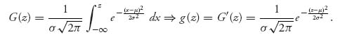
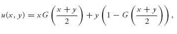
To illustrate a way to play this let’s take the mediated fair settlement to have a normal distribution with mean μ and variance σ2. The cumulative distribution function and density are given by
The condition for u(x, y) = xG(![]() ) + y (1 − G(
) + y (1 − G(![]() )) to have a saddle point becomes
)) to have a saddle point becomes
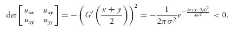
Therefore, any critical point is a saddle point, so we may apply the preceding.
The mean μ is the median for this distribution resulting in ![]() = μ. The spread between the union offer and the management offer should be
= μ. The spread between the union offer and the management offer should be
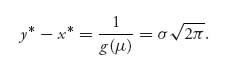
Solving the two linear equations y* + x* = 2μ, y* − x* = σ ![]() results in the offers by management x* = μ -σ
results in the offers by management x* = μ -σ ![]() and the union y* = μ + σ
and the union y* = μ + σ ![]() .
.
It is not true that every collection of payoff functions will have a pure Nash equilibrium, but there is at least one result guaranteeing that one exists. It should remind you of von Neumann’s minimax theorem, but it is more general than that because it doesn’t have to be zero sum. It also generalizes our previous statement of Nash’s theorem for bimatrix games.
Theorem 5.1.3 Let Q1 ![]()
![]() n and Q2
n and Q2 ![]()
![]() m be compact and convex sets.
m be compact and convex sets.
Then, there is a Nash equilibrium for (u1, u2).
2. Let Qi ![]()
![]() ni be convex and compact. If we have N payoff functions ui:Q1× Q2 × · · · × QN →
ni be convex and compact. If we have N payoff functions ui:Q1× Q2 × · · · × QN → ![]() , i = 1, 2, …, N, which are continuous and qi
, i = 1, 2, …, N, which are continuous and qi ![]() ui(qi, q−i) is concave, then there is a Nash equilibrium (q1*, …, qN*).
ui(qi, q−i) is concave, then there is a Nash equilibrium (q1*, …, qN*).
We will not prove this theorem but it again uses a fixed-point theorem. It indicates that if we do not have convexity of the strategy sets and concavity of the payoff functions, we may not have an equilibrium. It also says more than that. It gives us a way to set up mixed strategies for games that do not have pure Nash equilibria; namely, we have to convexify the strategy sets, and then make the payoffs concave in each variable. We do that by using continuous probability distributions instead of the discrete ones corresponding to mixed strategies for matrix games.
Getting back to the similarities with von Neumann’s minimax theorem, von Neumann’s theorem says roughly that a function f(x, y) that is concave in x and convex in y will have a saddle point. The connection with the Nash theorem is made by noticing that f(x, y) is the payoff for player I and −f(x, y) is the payoff for player II, and so if y ![]() f(x, y) is convex, then y
f(x, y) is convex, then y ![]() −f(x, y) is concave. So Nash’s result is a true generalization of the von Neumann minimax theorem. The Nash theorem is only a sufficient condition, not a necessary condition for a Nash equilibrium. In fact, many of the conditions in the theorem may be weakened, but we will not go into that here.
−f(x, y) is concave. So Nash’s result is a true generalization of the von Neumann minimax theorem. The Nash theorem is only a sufficient condition, not a necessary condition for a Nash equilibrium. In fact, many of the conditions in the theorem may be weakened, but we will not go into that here.
We conclude this section with several examples for finding Nash equilibria in N-person games.
Example 5.5 Mixed Strategies for 3-Person 2 × 2 Games. Suppose the game has three players in which each player will have a payoff function u1, u2, u3. Let’s label the three players I, II, and III. Then if each player uses a mixed strategy, X = (x1, x2), Y = (y1, y2), Z = (z1, z2), we have,
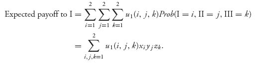
Similarly,
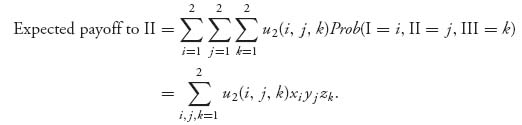
and
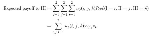
For example, suppose each player can choose Up or Down. We express the payoffs in matrix form as
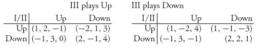
We will show that a mixed Nash Equilibrium is X* = (0.98159, 0.01841), Y* = (0.54869, 0.45131), Z* = (0.47720, 0.5228).
We use X = (x, 1-x), Y = (y, 1-y), Z = (z, 1-z) and have the payoffs
We are looking for an interior Nash equilibrium and there is no reason we can’t apply calculus for that. We have to solve the system of equations
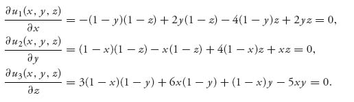
This is not an easy task to do by hand but Maple or Mathematica can do this easily. Two sets of solutions are found, but we readily eliminate the one with negative values and we get x = 0.98159, y = 0.54869, z = 0.47720.
Example 5.6 Tragedy of the Commons. There are many players consuming common resources, some of which may be renewable or nonrenewable. Typical examples of common resources include (1) fisheries in international waters, (2) ground water, (3) e-mail, (4) pollution, and so on.
Suppose there are N farmers who share grazing land for sheep. Each of the farmers has the option of keeping 1 sheep. The payoff to a farmer for having a sheep is 1, but sheep damage the common grazing land at cost −5 per sheep. Suppose each farmer has the payoff function
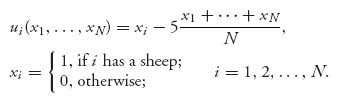
The total damage done to the grazing land is −5 times the number of sheep, but the damage is shared by all the farmers.
Now here is an amazing result. If N ≥ 5 a Nash equilibrium is (1, 1, …, 1), all the farmers should have a sheep and ui(1, 1, …, 1) = −4 for each farmer.
To see why this is true, if i decides to not have a sheep while everybody else sticks with their sheep, we have
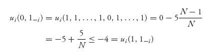
if and only if N ≥ 5.
The result is everybody loses a lot. Is there a way to avoid this outcome? One way is to impose a sheep tax. Let’s say the tax is α and this changes the payoffs to
![]()
Then, if everyone has a sheep ui(1, …, 1) = −4 − α. If α ≥ 1 it is easy to see that ui(0, 1−i) >-α, and so player i is better off getting rid of his sheep. Indeed, the new Nash equilibrium is (0, 0, …, 0), and no farmer has a sheep.
A Continuous Example Tragedy of the Commons. In this example, we again take the common resource to be grazing land for sheep but we assume farmers have a continuous number of sheep. There are two shepherds each of which has xi sheep, i = 1, 2. Sheep generate wool depending on how much grass they eat. Income for each shepherd is proportional to the wool they can sell so a reasonable payoff function representing the amount of wool generated depending on how many sheep the farmer owns is
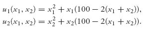
The second term takes into account that the grazing land can accommodate no more than 100 sheep. Taking partials and setting to zero gives
![]()
and, to be fair, each shepherd should graze 25 sheep, yielding ui(25, 25) = 625.
Suppose that the two shepherds meet in a bar before the grazing begins in order to come to an agreement about how many sheep each shepherd should graze. Naturally, they will assume that x1 = x2 or they begin with an unfair situation. Consequently, the payoff function of each player becomes
![]()
The maximum occurs at x = ![]() < 25. Together they should graze a total of about 33 sheep while without an agreement they would graze a total of 50 sheep. The payoff to each shepherd if they follow the agreement will be
< 25. Together they should graze a total of about 33 sheep while without an agreement they would graze a total of 50 sheep. The payoff to each shepherd if they follow the agreement will be
and this is strictly greater than 625, the amount they could get on their own. By cooperating both shepherds get a higher amount of wool. On the other hand, if you have up to 25 sheep to graze, you might think that you could sneak in a few more than ![]() to get a few more units of wool. Suppose you assume the other guy, say player 2, will go with the agreed upon
to get a few more units of wool. Suppose you assume the other guy, say player 2, will go with the agreed upon ![]() . What should you do then?
. What should you do then?
Your payoff is
which is maximized at x1 = ![]() , yielding shepherd 1 a payoff of
, yielding shepherd 1 a payoff of ![]() = 1111.11. Shepherd 1 definitely has an incentive to cheat. So does shepherd 2. Unless there is some penalty for violating the agreement, each player will end up grazing their Nash equilibrium.
= 1111.11. Shepherd 1 definitely has an incentive to cheat. So does shepherd 2. Unless there is some penalty for violating the agreement, each player will end up grazing their Nash equilibrium.
In general, take any game with a profit function of the form
![]()
where c is a unit cost and f(·) is a function giving the unit return to grazing. It is assumed that f is a decreasing function of the total sheep grazing to reflect the overgrazing effect. The result will illustrate a tragedy of the commons effect.
Example 5.7 Consumption Over Two Periods. Suppose we have a two period consumption problem. If we have two players consuming xi, i = 1, 2 units of a resource today, then they have to take into account that they will also consume the resource tomorrow. Suppose the total amount of the resource is M > 0. On day 1, we must have x1 + x2 ≤ M. However, since the players act independently, it is possible they will choose x1 + x2 > M in which case we will set x1 = x2 = ![]() .
.
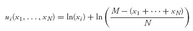
On day 2, the amount of resource available is M−(x1 + x2) and we assume that each player will get half of the amount available at that time. Each player only decides how much they consume today, but they have to take into account tomorrow as well. Now let’s set up each player’s payoff function. For player i = 1, 2,
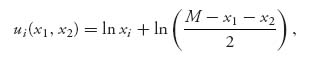
where we measure the utility of consumption using an increasing but concave down function. This is a typical payoff function illustrating diminishing returns—a dollar more when you have a lot of them is not going to bring you a lot of pleasure. Another point to make is that a player chooses to consume xi in period one, and then equally shares the remaining amount of resource in period 2. Anyone who doesn’t like to share has an incentive to consume more in period one.
Let’s assume that 0 < x1 + x2 < M. Then
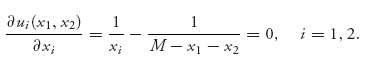
Consider player 1. We solve the condition for x1 as a function of x2 to obtain the best response function for player 1 given by
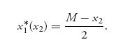
Similarly, x2* (x1) = ![]() . If we plot these two lines in the x1 − x2 plane, we see that they cross when x1* = x2* =
. If we plot these two lines in the x1 − x2 plane, we see that they cross when x1* = x2* = ![]() . This is the Nash equilibrium. They consume together
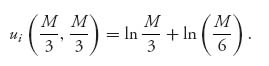
. This is the Nash equilibrium. They consume together ![]() M in the first period and defer one-third for the next period. The payoff to each player is then
M in the first period and defer one-third for the next period. The payoff to each player is then
Next, we consider what happens if the players act as one for the entire problem. In other words, they seek to maximize their total payoffs as a function of (x1, x2). The problem becomes
![]()
Maximizing the sum of the payoffs is called looking for the social optimum. Assuming 0 < x1 + x2 < M, we again take derivatives and set to zero to get
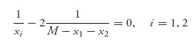
which results in
![]()
as the social optimum amount of consumption. Acting together, they each consume half the resource in period one. Why do they do that?
We can generalize this to N > 2 players quite easily.
Suppose that M is the total amount of a common resource available and let xi, i = 1, 2, …, N denote the amount player i consumes in period one. We must have
![]()
By convention, if x1 + · · · + xN > M we take xi = ![]() . Tomorrow the amount of consumption for each player is set as
. Tomorrow the amount of consumption for each player is set as ![]() which means they get an equal share of what’s left over after the first days consumption.
which means they get an equal share of what’s left over after the first days consumption.
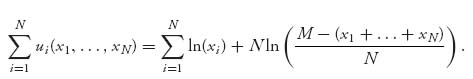
Next, the utility of consumption is given by
Then, player i’s goal is to

Assuming we have an interior maximum we can find the best response function by taking derivatives:
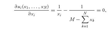
which implies xi* (x1, x2, …, xi−1, xi + 1, …, xN) = ![]() (M −
(M − ![]() . By symmetry, we get
. By symmetry, we get
This means that each consumer uses up ![]() of the resources today, and then
of the resources today, and then ![]() of the resource tomorrow.
of the resource tomorrow.
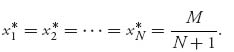
Now we compare what happens if the consumers share the resource agreeing to maximize their benefits as a group instead of independently. In this case, we maximize the social optimum:
Solving this system results in the social optimum point x1* = · · · = xN* = ![]() . Note that as N → ∞ the social optimum amount of consumption in period one approaches zero. If a player gives up a unit of consumption in period one, then the player has to share that unit of consumption with everyone in period two.
. Note that as N → ∞ the social optimum amount of consumption in period one approaches zero. If a player gives up a unit of consumption in period one, then the player has to share that unit of consumption with everyone in period two.
Our next example has had far reaching implications to many areas but especially transportation problems. Did you ever think that adding a new road to an already congested system might makes things worse?
FIGURE 5.2 Braess paradox.
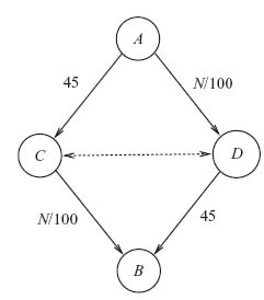
Example 5.8 Braess’s Paradox. In this example, we will consider an N-person nonzero sum game in which each player wants to minimize a cost. The problem will add a resource that should allow the players to reduce their cost, but in fact makes things worse. This is a classic example called Braess’s paradox.3
Refer to Figure 5.2. There are N commuters who want to travel from A to B. The travel time on each leg depends on the number of commuters who choose to take that leg. Note that if a commuter chooses A → D → B the initial choice of leg determines automatically the second leg before the zip road is added. The travel times are as follows:
- A → D and C → B is N/100.
- A → C and D → B is 45.
Each player wants to minimize her own travel time, which is taken as the payoff for each player.
The total travel time for each commuter A → D → B is N/100 + 45, and the total travel time A → C → B is also N/100 + 45. If one of the routes took less time, any commuter would switch to the quicker route. Thus, the only Nash equilibrium is for exactly N/2 players to take each route (assuming N is even, what if N is odd?). For example, if N = 2000 then the travel time under equilibrium is 55 and 1000 choose A → D → B and 1000 choose A → C → B. This assumes perfect information for all commuters.
Now if a zip road (the dotted line) from C ![]() D is built which takes essentially no travel time, then consider what a rational driver would do. We’ll take N = 2000 for now. Since N/100 = 20 < 45 all drivers would choose initially A → D. When the driver gets to D, a commuter would take the zip road to C and then take C → B. This results in a total travel time of N/100 + N/100 = 40 < 55, and the zip road saves everyone 15.
D is built which takes essentially no travel time, then consider what a rational driver would do. We’ll take N = 2000 for now. Since N/100 = 20 < 45 all drivers would choose initially A → D. When the driver gets to D, a commuter would take the zip road to C and then take C → B. This results in a total travel time of N/100 + N/100 = 40 < 55, and the zip road saves everyone 15.
But is this always true no matter how many commuters are on the roads? Actually, no. For example, if N = 4000 then all commuters would pick A → D and this would take N/100 = 40 < 45; then they would take the zip road to C and travel from C → B. The total commute time would be 80. If they skip the zip road, their travel time would be 40 + 45 = 85 < 80, so they will take the zip road. On the other hand, if the zip road did not exist, half the commuters would take A → D → B and the other half would take A → C → B, with a travel time of 45 + 20 = 65 < 80. Giving the commuters a way to cross over actually makes things worse! Having an option and assuming commuters always do what’s best for them results in longer travel time for everyone.
Braess’s paradox has been seen in action around the world and traffic engineers are well aware of the paradox. Moreover, this paradox has applications to much more general networks in computer science and telecommunications. It should be noted that this is not really a paradox since it has an explanation, but it is completely counterintuitive.
Our next two examples show what happens when players think through the logical consequences.
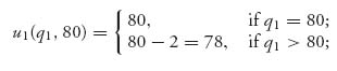
Example 5.9 The Traveler’s Paradox.4 Two airline passengers who have luggage with identical contents are informed by the airline that their luggage has been lost. The airline offers to compensate them if they make a claim in some range acceptable to the airline. Here are the payoff functions for each player:
It is assumed that the acceptable range is [a, b] and qi ![]() [a, b], i = 1, 2. The idea behind these payoffs is that if the passengers’ claims are equal the airline will pay the amount claimed. If passenger I claims less than passenger II, q1 < q2, then passenger II will be penalized an amount R and passenger I will receive the amount she claimed plus R. Passenger II will receive the lower amount claimed minus R. Similarly, if passenger I claims more than does passenger II, q1 > q2, then passenger I will receive q2 − R, and passenger II will receive the amount claimed q2 + R.
[a, b], i = 1, 2. The idea behind these payoffs is that if the passengers’ claims are equal the airline will pay the amount claimed. If passenger I claims less than passenger II, q1 < q2, then passenger II will be penalized an amount R and passenger I will receive the amount she claimed plus R. Passenger II will receive the lower amount claimed minus R. Similarly, if passenger I claims more than does passenger II, q1 > q2, then passenger I will receive q2 − R, and passenger II will receive the amount claimed q2 + R.
Suppose, to be specific, that a = 80, b = 200, so the airline acceptable range is from $80 to $200. We take R = 2, so the penalty is only $2 for claiming high. Believe it or not, we will show that the Nash equilibrium is (q1 = 80, q2 = 80) so both players should claim the low end of the airline range (under the Nash equilibrium concept). To see that, we have to show that
![]()
for all 80 ≤ q1, q2 ≤ 200. Now
and
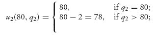
So indeed (80, 80) is a Nash equilibrium with payoff 80 to each passenger. But clearly, they can do better if they both claim q1 = q2 = $200. Why don’t they do that? The problem is that there is an incentive to undercut the other traveler. If R is $2, then, if one of the passengers drops her claim to $199, this passenger will actually receive $201. This cascades downward, and the undercutting disappears only at the lowest range of the acceptable claims. Do you think that the passengers would, in reality, make the lowest claim?
Example 5.10 Guessing Two-Thirds of the Average. A common game people play is to choose a number in order to match some objective, usually to guess the number someone is thinking, as close as possible. In a group of people playing this game, the closest number wins. We consider a variation of this game that seems much more difficult for everyone involved.
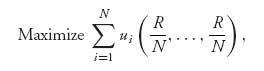
Suppose we have three people who are going to choose an integer from 1 to N. The person who chooses closest to two-thirds of the average of all the numbers chosen wins $1. If two or more people choose the same number closest to two-thirds of the average, they split the $1. We set up the payoff functions as follows:
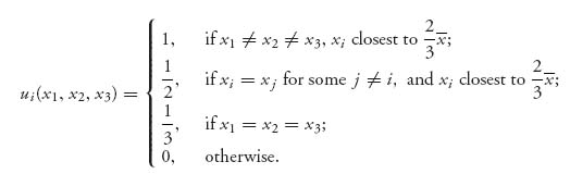
Here ![]() . The possible choices for xi are { 1, 2, …, N}.
. The possible choices for xi are { 1, 2, …, N}.
The claim is that (x1*, x2*, x3*) = (1, 1, 1) is a Nash equilibrium in pure strategies. All the players should call 1 and they each receive ![]() .
.
To see why this is true let’s consider player 1. The rest would be the same. We must show
![]()
Suppose player 1 chooses x1 = k ≥ 2. Then
![]()
and the distance between two-thirds of the average and k is
If player 1 had chosen x1 = 1, the distance from 1 to two-thirds of the average is |1 − ![]() | =
| = ![]() . We ask ourselves if there is a k > 1 so that |
. We ask ourselves if there is a k > 1 so that |![]() k−
k−![]() | <
| < ![]() ? The answer to that is no as you can easily check. In a similar way, we show that none of the players do better by switching to another integer and conclude that (1, 1, 1) is a Nash equilibrium.
? The answer to that is no as you can easily check. In a similar way, we show that none of the players do better by switching to another integer and conclude that (1, 1, 1) is a Nash equilibrium.
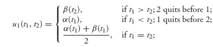
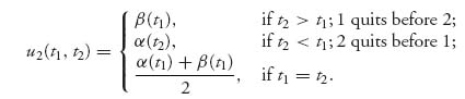
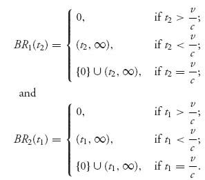
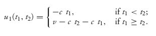
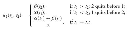
Example 5.11 War of Attrition. A game called the war of attrition game in which two countries compete for a resource which they each value at v. The players incur a cost of c per unit time for continuing the war for the resource but they may choose to quit at any time. For each player, the payoff functions are taken to be
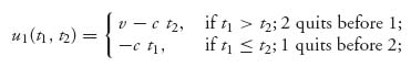
and
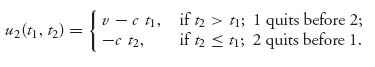
One way to find the pure Nash equilibrium, if any, is to find the best response functions (which are sets in general) and see where they intersect.
It is not hard to check that
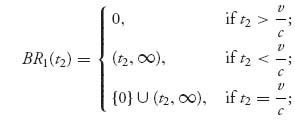
and
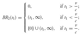
By graphing these set valued functions on the same set of axes in the t1 − t2 plane we obtain
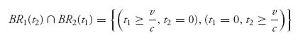
and these are the pure Nash equilibria.The payoffs of the countries are as follows:
![]()
This means that a pure Nash equilibrium involves one of the two countries stopping immediately. Note too that if one player stops immediately, any time after ![]() is the other player’s part of the Nash equilibrium. But this seems a little unrealistic and certainly doesn’t seem to be what happens in practice.
is the other player’s part of the Nash equilibrium. But this seems a little unrealistic and certainly doesn’t seem to be what happens in practice.
The war of attrition game raises the question if there are any mixed strategies as Nash equilibria, and how do we find them. Time for a little aside.
Do We Have Mixed Strategies in Continuous Games?5
How do we set up the game when we allow mixed strategies and we have a continuum of pure strategies? This is pretty straightforward but the analysis of the game is not. Here is a sketch of what we have to do. Consider only two players with payoff functions u1: Q1 × Q2 → ![]() and u2:Q1 × Q2 →
and u2:Q1 × Q2 → ![]() , where Q1
, where Q1 ![]()
![]() n, Q2
n, Q2 ![]()
![]() m are the pure strategy sets for each player. For simplicity let’s assume n = m = 1.
m are the pure strategy sets for each player. For simplicity let’s assume n = m = 1.
A mixed strategy for player I is now a probability distribution on Q1, but since Q1 has a continuum of points, this means that a mixed strategy is a probability density function which we label X(x). That is a function X(x) ≥ 0 and ∫Q1 X(x) dx = 1. 6 Similarly, a mixed strategy for player II is a probability density function Y(y) on Q2 with Y(y) ≥ 0, ∫Q2Y(y) dy = 1. Intuitively X(x) represents Prob(I plays x) but more accurately
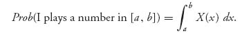
Given choices of mixed strategies X, Y we then calculate the expected payoff for player I as
and
for player II.
It may be proved that there is a Nash equilibrium in mixed strategies under mild assumptions on u1, u2, Q1, Q2. For example, if the payoff functions are continuous and Qi are convex and compact then a Nash equilibrium is guaranteed to exist. The question is how to find it, because now we are looking for functions X, Y, not points or vectors. The only method we present here for finding the Nash equilibrium (or saddle point if u2 = −u1) is based on the Equality of Payoffs theorem.
Proposition 5.1.4 Let X* (x), Y* (y) be Nash equilibrium probability density functions. Assume the payoff functions are upper semicontinuous in each variable.7
If x0 ![]() Q1 is a point where X* (x0) > 0, then
Q1 is a point where X* (x0) > 0, then
If y0 ![]() Q2 is a point where Y* (y0) > 0, then
Q2 is a point where Y* (y0) > 0, then
![]()
In particular, if X* (x) > 0 for all x ![]() Q1, then x
Q1, then x ![]() EI (x, Y) is a constant and that constant is EI (X*, Y*). Similarly, if Y* (y) > 0 for all y
EI (x, Y) is a constant and that constant is EI (X*, Y*). Similarly, if Y* (y) > 0 for all y ![]() Q2, then y
Q2, then y ![]() EII (X*, y) is a constant and that constant is EII(X*, Y*).
EII (X*, y) is a constant and that constant is EII(X*, Y*).
Proof We will only show the first statement. Since X*, Y* is a Nash equilibrium, vI ≥ EI(x, Y*) for all x ![]() Q1, and in particular, this is true for x = x0. Now suppose that vI > EI (x0, Y*), then, by upper semicontinuity, this must be true on a neighborhood N
Q1, and in particular, this is true for x = x0. Now suppose that vI > EI (x0, Y*), then, by upper semicontinuity, this must be true on a neighborhood N![]() Q1 of x0. Thus we have, by integrating over the appropriate sets,
Q1 of x0. Thus we have, by integrating over the appropriate sets,
and
The last strict inequality holds because X* (x0) > 0 and hence X* (x) > 0 on N. Adding the two inequalities, we get
a contradiction. ![]()
Example 5.12 Consider8 the war of attrition game in Example 5.11. We saw there that the pure Nash equilibria are as follows:
![]()
Next, we see if there is a mixed Nash equilibrium. We use Proposition 5.1.4 and assume that the density function for player I’s part of the Nash equilibrium satisfies X* (t1) > 0. In that case we know that for player II’s density function Y*, we have for all 0 ≤ t2 < ∞,

Since this is true for any t1, we take the derivative of both sides with respect to t1 to get, using the fundamental theorem of calculus
Again take a derivative with respect to t1 to see that
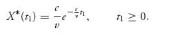
This is a first-order ordinary differential equation for Y*, which may be solved by integration to see that
![]()
where C is a constant determined by the condition ∫0∞ Y* (y) dy = 1. We determine that C = ![]() , and hence, the density is
, and hence, the density is
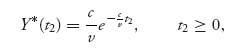
which is an exponential density for an exponentially distributed random variable representing the time that player II will quit with mean ![]() . Since the players in this game are completely symmetric, it is easy to check that
. Since the players in this game are completely symmetric, it is easy to check that
Now suppose we want to know the expected length the war will last. To answer that question just requires a little probability. First, let τ denote the random variable giving the length of the war and let τi, i = 1, 2, be the random variable that gives the time each player will quit. The war goes on until time τ = min { τ1, τ2}. Then from what we just found
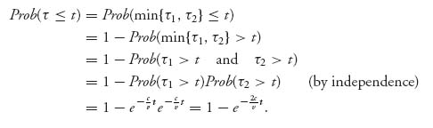
This tells us that τ has a density ![]() e−
e−![]() t and hence is also exponentially distributed with mean
t and hence is also exponentially distributed with mean ![]() . Because each player would quit on average at time
. Because each player would quit on average at time ![]() you might expect that the war would last the same amount of time, but that is incorrect. On average, the time the first player quits is half of the time either would quit.
you might expect that the war would last the same amount of time, but that is incorrect. On average, the time the first player quits is half of the time either would quit.
Next, we want to calculate the expected payoffs to each player if they are playing their Nash equilibrium. This is a straightforward calculation:
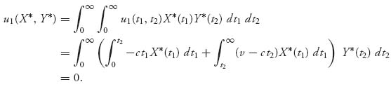
Similarly, the expected payoff to player 2 is also zero when the optimal strategies are played.
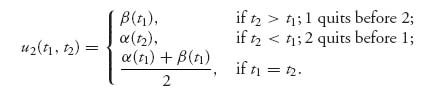
The war of attrition is a particular example of a game of timing. In general, we have two functions α (t), β (t) and payoff functions depending on the time that each player chooses to quit. In particular, we take the strategy sets to be [0, 1] for both players and
and
If we take α and β to be continuous, decreasing functions with α (t) < β (t) and α (0) > β (1), then the general war of attrition has two pure Nash equilibria given by { (t1 = τ*, t2 = 0), (t1 = 0, t2 = τ*)} where τ* > 0 is the first time where b(τ*) = a(0).
These payoff functions are not continuous so that any Nash equilibria found must be verified to really be Nash points.
Mixed strategies for continuous games can be very complicated. They may not have continuous densities and generally should be viewed as general cumulative distribution functions. This is a topic for a much more advanced course and so we stop here.
Problems
5.1 This problem makes clear the connection between a pair of numbers (q1*, q2*) that maximizes both payoff functions and a Nash equilibrium. Suppose that we have a two-person game with payoff functions ui(q1, q2), i = 1, 2. Suppose there is a pure strategy pair (q1*, q2*) that maximizes both u1 and u2 as functions of the pair (q1, q2).
5.2 Consider the zero sum game with payoff function for player 1 given by u(x, y) = −2x2 + y2 + 3xy−x−2y, 0 ≤ x, y ≤ 1. Show that this function is concave in x and convex in y. Find the saddle point and the value.
5.3 The payoff functions for Curly and Shemp are, respectively,
![]()
with x ![]() [1, 3], y
[1, 3], y ![]() [1, 3]. Curly chooses x and Shemp chooses y.
[1, 3]. Curly chooses x and Shemp chooses y.
5.4 Consider the game in which two players choose nonnegative integers no greater than 1000. Player 1 must choose an even integer, while player 2 must choose an odd integer. When they announce their number, the player who chose the lower number wins the number she announced in dollars. Find the Nash equilibrium.
5.5 In the tragedy of the commons Example 5.6, we saw that if N ≥ 5 everyone owning a sheep is a Nash equilibrium. Analyze the case N ≤ 4.
5.6 There are N players each using ri units of a resource whose total value is R = ![]() . The cost to player i for using ri units of the resource is f(ri) + g(R − ri) where we take f(x) = 2x2, g(x) = x2. This says that a player’s cost is a function of the amount of the total used by that player and a function of the amount used by the other players. The revenue player i receives from using ri units is h(ri), where h(x) =
. The cost to player i for using ri units of the resource is f(ri) + g(R − ri) where we take f(x) = 2x2, g(x) = x2. This says that a player’s cost is a function of the amount of the total used by that player and a function of the amount used by the other players. The revenue player i receives from using ri units is h(ri), where h(x) = ![]() . Assume that the total resources used by all players is not unlimited so that 0 ≤ R ≤ R0 < ∞.
. Assume that the total resources used by all players is not unlimited so that 0 ≤ R ≤ R0 < ∞.
over R ≥ 0. Practically, this means that the players do not act independently but work together so that the total payoffs to all players is maximized. Find the value of R that provides the maximum, Rs, and find it’s value when N = 12.
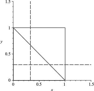
5.7 Consider the median voter model Example 5.3. Let X denote the preference of a voter and suppose X has density f(x) = −1.23x2 + 2x + 0.41, 0 ≤ x ≤ 1. Find the Nash equilibrium position a candidate should take in order to maximize their voting percentage.
5.8 In the arbitration game Example 5.4, we have seen that the payoff function is given by
where G is a cumulative distribution function.
![]()
Assume that the minimum offer must be at least a > 0 and find the smallest possible a > 0 so that the offers are positive. In other words, the range of offers is X + a and X has an exponential distribution.
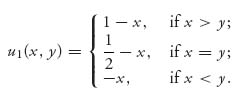
5.9 Consider the game in which player I chooses a nonnegative number x, and player II chooses a nonnegative number y (x and y are not necessarily integers). The payoffs are as follows:
![]()
Determine player I’s best response x(y) to a given y, and player II’s best response y(x) to a given x. Find a Nash equilibrium, and give the payoffs to the two players.
5.10 Two players decide on the amount of effort they each will exert on a project. The effort level of each player is qi ≥ 0, i = 1, 2. The payoff to each player is
![]()
where c > 0 is a constant. This choice of payoff models a synergistic effect between the two players.
5.11 Suppose two citizens are considering how much to contribute to a public playground, if anything. Suppose their payoff functions are given by
![]()
where wi is the wealth of player i. This payoff represents a benefit from the total provided for the playground q1 + q2 by both citizens, the amount of wealth left over for private benefit wi − qi, and an interaction term (wi − qi)(q1 + q2) representing the benefit of private money with the amount donated. Assume w1 = w2 = w and 0 ≤ qi ≤ w. Find a pure Nash equilibrium.
5.12 Consider the war of attrition game in Example 5.11. Verify that
![]()
Find the payoff for country 2 and find the pure Nash equilibrium.
5.13 This problem considers the War of Attrition but with differing costs of continuing the war and differing values placed upon the resource over which the war is fought. Country 1 places value v1 on the land, and country 2 values it at v2. The players choose the time at which to concede the land to the other player, but there is a cost for letting time pass. Suppose that the cost to each country is ci, i = 1, 2 per unit of time. The first player to concede yields the land to the other player at that time. If they concede at the same time, each player gets half the land. Determine the payoffs to each player and determine the pure Nash equilibria.
5.14 Consider the general war of attrition as described in this section with given functions α, β. The payoff functions are as follows:
and
Verify that if we take α and β to be continuous, decreasing functions with α (t) < β (t) and α (0)>β (1), then the general war of attrition has two pure Nash equilibria given by { (t1 = τ*, t2 = 0), (t1 = 0, t2 = τ*)} where τ* > 0 is the first time where β (τ*) = α (0).
5.15 This is an exercise on Braess’s paradox. Consider the traffic system in which travelers want to go from A → C. The travel time for each car depends on the total traffic.
Braess’s paradox.
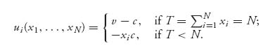
5.16 We have a game with N ≥ 2 players. Each player i must simultaneously decide whether to join the team or not. If player i joins then xi = 1 and otherwise xi = 0. Let T = ![]() xi denote the size of the team. If player i doesn’t join the team, then player i receives a payoff of zero. If player i does join the team then i pays a cost of c. If all N players join the team, so that T = N, then each player enjoys a benefit of v. Hence, player i’s payoff is
xi denote the size of the team. If player i doesn’t join the team, then player i receives a payoff of zero. If player i does join the team then i pays a cost of c. If all N players join the team, so that T = N, then each player enjoys a benefit of v. Hence, player i’s payoff is
Suppose that v > c > 0.
5.17 Two companies are at war over a market with a total value of V > 0. Company 1 allocates an effort x > 0, and company 2 allocates an effort y > 0 to obtain all or a portion of V. The portion of V won by company 1 if they allocate effort x is ![]() V at cost C1x, where C1 > 0 is a constant. Similarly, the portion of V won by company 2 if they allocate effort y is
V at cost C1x, where C1 > 0 is a constant. Similarly, the portion of V won by company 2 if they allocate effort y is ![]() V at cost C2y, where C2 > 0 is a constant. The total reward to each company is then
V at cost C2y, where C2 > 0 is a constant. The total reward to each company is then
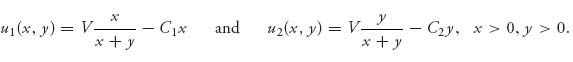
Show that these payoff functions are concave in the variable they control and then find the Nash equilibrium using calculus.
5.18 Suppose that a firm’s output depends on the number of laborers they have hired. Let p = number of workers, w = worker compensation (per unit time) and assume
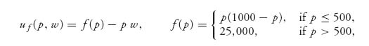
is the payoff to the firm if they hire p workers and pay them w. Assume that the union payoff is uu(p, w) = p, w.
Find the best response for the firm to a wage demand assuming wm ≤ w ≤ W. Then find w to maximize uu(p(w), w). This scheme says that the firm will hire the number of workers that maximizes its payoff for a given wage. Then the union, knowing that the firm will use its best response, will choose a wage demand that maximizes its payoff assuming the firm uses p(w).
5.19 Suppose that N > 2 players choose an integer in { 1, 2, …, 100}. The payoff to each player is 1 if that player has chosen an integer which is closest to ![]() of the average of the numbers chosen by all the players. If two or more players choose the closest integer, then they equally split the 1. The payoff of other players is 0. Show that the Nash equilibrium is for each player to choose the number 1.
of the average of the numbers chosen by all the players. If two or more players choose the closest integer, then they equally split the 1. The payoff of other players is 0. Show that the Nash equilibrium is for each player to choose the number 1.
5.20 Two countries share a long border. The pollution emitted by one country affects the other. If country i = 1, 2 pollutes a total of Qi tons per year, they will emit pi tons per year into the atmosphere, and clean up Qi − pi tons per year (before it is emitted) at cost c dollars per ton. Health costs attributed to the atmospheric pollution are proportional to the square of the total atmospheric pollution in each country. The total atmospheric pollution in country 1 is p1 + kp2, and in country 2 it is p2 + k p1. The constant 0 < k < 1 represents the fraction of the neighboring country’s pollution entering the atmosphere. Assume the proportionality constants and cost of cleanup is the same for both countries.
5.21 Corn is a food product in high demand but also enjoys a government price subsidy. Assume that the demand for corn (in bushels) is given by D(p) = 150, 000(15 – p)+, where p is the price per bushel. The government program guarantees that p ≥ 2. Suppose that there are three corn producers who have reaped 1 million bushels each. They each have the choice of how much to send to market and how much to use for feed (at no profit). Find the Nash equilibrium. What happens if one farmer sends the entire crop to market?
5.22 This is known as the division of land game. Suppose that there is a parcel of land as in the following figure:
Division of land.
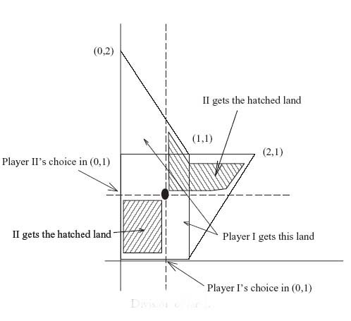
Player I chooses a vertical line between (0, 1) on the x-axis and player II chooses a horizontal line between (0, 1) on the y-axis. Player I gets the land below II’s choice and right of I’s choice as well as the land above II’s choice and left of I’s line. Player II gets the rest of the land. Both players want to choose their line so as to maximize the amount of land they get.
5.23 A famous economics problem is called the Samaritan’s Dilemma. In one version of this problem, a citizen works in period 1 at a job giving a current annual net income of I. Out of her income she saves x for her retirement and earns r% interest per period. When she retires, considered to occur at period 2, she will receive an annual amount y from the government. The payoff to the citizen is
![]()
where u1 is the first-period utility function, and is increasing but concave down, and u2 is the second-period utility function, that is also increasing and concave down. These utility functions model increasing utility but at a diminishing rate as time progresses. The constant δ > 0, called a discount rate, finds the present value of dollars that are not delivered until the second period. The government has a payoff function
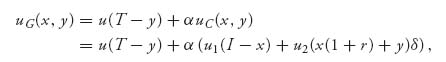
where u(t) is the government’s utility function for income level T, such as tax receipts, and α > 0 represents the factor of benefits received by the government for a happy citizen, called an altruism factor.
5.24 Suppose we have a zero sum game and mixed densities X0 for player I and Y0 for player II.
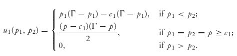
5.25 Two investors choose investment levels from the unit interval. The investor with the highest level of investment wins the game, which has payoff 1 but costs the level of investment. If the same level of investment is chosen, they split the market. Take the investment levels to be x ![]() [0, 1] for player I and y
[0, 1] for player I and y ![]() [0, 1] for player II. Investor I’s payoff function is
[0, 1] for player II. Investor I’s payoff function is
is a constant, vI, independent of x (assuming f(x) > 0). Take the derivative of both sides with respect to x and solve for the density g(x) for player II. Do a similar procedure to find the density for player I. Now find vI and vII.
5.2 Economics Applications of Nash Equilibria
The majority of game theorists are economists (or some combination of economics and mathematics), and in recent years many winners of the Nobel Prize in economics have been game theorists (Aumann9, Harsanyi10, Myerson11, Schelling12, Selten 13, and, of course, Nash, to mention a only a few. Nash, however, would probably consider himself primarily a pure mathematician. In 2012 Lloyd Shapley and Alvin Roth became the latest game theorists to be awarded the Nobel Prize). In this section, we discuss some of the basic applications of game theory to economics problems.
5.2.1 COURNOT DUOPOLY
Cournot14 developed one of the earliest economic models of the competition between two firms. Suppose that there are two companies producing the same gadget. Firm i = 1, 2 chooses to produce the quantity qi ≥ 0, so the total quantity produced by both companies is q = q1 + q2.
We assume in this simplified model that the price of a gadget is a decreasing function of the total quantity produced by the two firms. Let’s take it to be
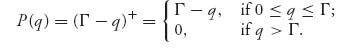
Γ represents the price of gadgets beyond which the quantity to produce is essentially zero, and the price a consumer is willing to pay for a gadget if there are no gadgets on the market. Suppose also that to make one gadget costs firm i = 1, 2, ci dollars per unit so the total cost to produce qi units is ciqi, i = 1, 2.
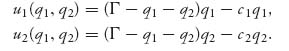
The total quantity of gadgets produced by the two firms together is q1 + q2, so that the revenue to firm i for producing q1 units of the gadget is qiP(q1 + q2). The cost of production to firm i is ciqi. Each firm wants to maximize its own profit function, which is total revenue minus total costs and is given by
Observe that the only interaction between these two profit functions is through the price of a gadget which depends on the total quantity produced.
Let’s begin by taking the partials and setting to zero. We assume that the optimal production quantities are in the interval (0, Γ):
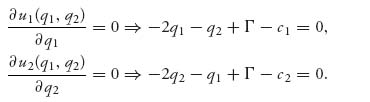
Note that we take the partial of ui with respect to qi, not the partial of each payoff function with respect to both variables. We are not trying to maximize each profit function over both variables, but each profit function to each firm as a function only of the variable they control, namely, qi. That is a Nash equilibrium. Solving each equation gives the best response functions
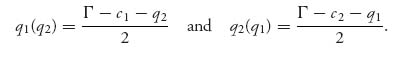
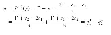
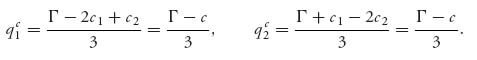
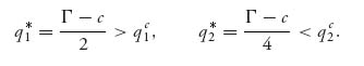
Now the intersection of these two best responses gives the optimal production quantities for each firm at
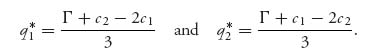
We will have q1* > 0 and q2* > 0 if we have Γ > 2 c1, Γ > 2 c2.
Now we have to check the second-order conditions to make sure we have a maximum. At these points, we have
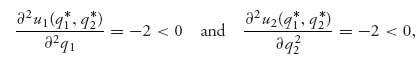
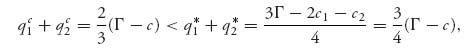
and so (q1*, q2*) are values that maximize the profit functions, when the other variable is fixed. The total amount the two firms should produce is
![]()
and Γ > q* > 0 if Γ > 2 c1, Γ > 2 c2. We see that our assumption about where the optimal production quantities would be found was correct if Γ is large enough. If, however, say Γ < 2 c1 − c2 then the formula for q1* < 0 and since the payoffs are concave down, the Nash equilibrium point is then q1* = 0, q2* = ![]() . For the remainder of this section, we assume Γ > 2 c1, Γ > 2 c2.
. For the remainder of this section, we assume Γ > 2 c1, Γ > 2 c2.
The price function at the quantity q* is then
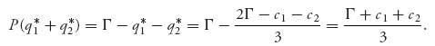
That is the market price of the gadgets produced by both firms when producing optimally.
Turn it around now and suppose that the price of gadgets is set at
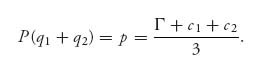
If this is the market price of gadgets how many gadgets should each firm produce? The total quantity that both firms should produce (and will be sold) at this price is q = P−1(p), or
We conclude that the quantity of gadgets sold (demanded) will be exactly the total amount that each firm should produce at this price. This is called a market equilibrium and it turns out to be given by the Nash point equilibrium quantity to produce. In other words, in economics, a market equilibrium exists when the quantity demanded at a price p is q1* + q2* and the firms will optimally produce the quantities q1*, q2* at price p. That is exactly what happens when we use a Nash equilibrium to determine q1*, q2*.
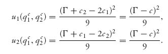
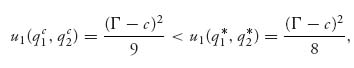
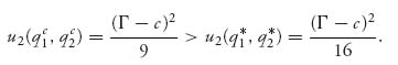
Finally, substituting the Nash equilibrium point into the profit functions gives the equilibrium profits
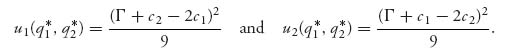
Note that the profit of each firm depends on the costs of the other firm. That’s a problem because how is a firm supposed to know the costs of a competing firm? The costs can be estimated, but known for sure...? This example is only a first-cut approximation, and we will have a lot more to say about this later.
5.2.2 A SLIGHT GENERALIZATION OF COURNOT
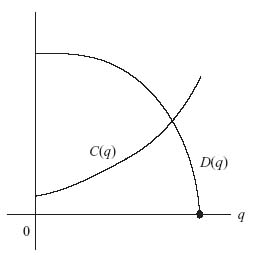
Suppose that price is a function of the demand, which is a function of the total supply q of gadgets, so P = D(q) and D is the demand function. We assume that if q gadgets are made, they will be sold at price P = D(q). Suppose also that C(z) is the cost to the two firms if z units of the gadget are produced. Again, each firm is trying to maximize its own profit, and we want to know how many gadgets each firm should produce. Another famous economist (A. Wald15) solved this problem (as presented in Parthasarathy and Raghavan (1971)). Figure 5.3 shows the relationship of of the demand and cost functions.
FIGURE 5.3 Demand and cost functions.
The next theorem generalizes the Cournot duopoly example to cases in which the price function and the cost functions are not necessarily linear. But we have to assume that they have the same cost function.
Theorem 5.2.1 Suppose that P = D(q) has two continuous derivatives, is nonincreasing, and is concave in the interval 0 ≤ q ≤ Γ, and suppose that
![]()
This means there is a positive demand if there are no gadgets, but the demand (or price) shrinks to zero if too many gadgets are on the market. Also, P = D(q), the price per gadget decreases as the total available quantity of gadgets increases. Suppose that firm i = 1, 2 has Mi ≥ Γ gadgets available for sale.
Suppose that the cost function C has two continuous derivatives, is strictly increasing, nonnegative, and convex, and that C′(0) < D(0). The payoff functions are again the total profit to each firm:
![]()
Then, there is one and only one Nash equilibrium given by (q*, q*), where q* ![]() [0, Γ] is the unique solution of the equation
[0, Γ] is the unique solution of the equation
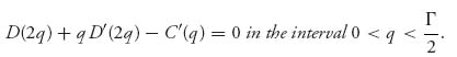
Under our assumptions, both firms produce exactly the same amount q* ![]() (0,
(0, ![]() k) and each receives the same profit u1(q*, q*) = u2(q*, q*). If they had differing cost functions, this would not be true.
k) and each receives the same profit u1(q*, q*) = u2(q*, q*). If they had differing cost functions, this would not be true.
Sketch of the Proof. By the assumptions we put on D and C, we may apply the theorem that guarantees that there is a Nash equilibrium to know that we are looking for something that exists. Call it (q1*, q2*). We assume that this will happen with 0 < q1* + q2* < Γ. By taking the partial derivatives and setting equal to zero, we see that
and
We solve these equations by subtracting to get
Remember that C′′ (q) ≥ 0 (so C′ is increasing) and D′ < 0. This means that if q1* < q2*, then we have the sum of two positive quantities in (5.2) adding to zero, which is impossible. So, it must be true that q1* ≥ q2*. However, by a similar argument, strict inequality would be impossible, and so we conclude that q1* = q2* ≡ q*. Actually, this should be obvious because the firms are symmetric and have the same costs.
So now we have

In addition, it is not too difficult to show that q* is the unique root of this equation (and therefore the only stationary point). That is the place where the assumption that C′(0) < D(0) is used. Finally, by taking second derivatives, we see that
for each payoff function, and hence the unique root of the equation is indeed a Nash equilibrium. ![]()
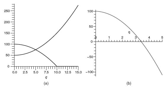
Example 5.13 Let’s take D(q) = 100 − q2, 0 ≤ q ≤ 10, and cost function C(q) = 50 + q2. Then C′(0) = 0 < D(0) = 100, and the functions satisfy the appropriate convexity assumptions. Then q is the unique solution of
![]()
in the interval 0 < q < 10. The unique solution is given by q* = 3.413. The unit price at this quantity should be D(2q*) = 88.353, and the profit to each firm will be ui(q*, q*) = q* D(2q*) − C(q*) = 120.637. These numbers, as well as some pictures, can be obtained using the Maple commands:
 > restart:
 > De: = q- > piecewise(q < 10, 100-q ^2, q > = 10, 0);
 > C: = q- > 50 + q^2;
 > plot(De(q), C(q), q = 0..15, color = [red, green]);
 > diff(De(q), q);
 > a: = eval(%, [q = 2*q]);
 > qstar: = fsolve(De(2*q) + q*a-diff(C(q), q) = 0, q);
 > plot(De(2*q) + q*a-diff(C(q), q), q = 0..5);
 > De(qstar);
 > qstar*De(2*qstar)-C(qstar);
This will give you a plot of the demand function and cost function on the same set of axes, and then a plot of the function giving you the root where it crosses the q-axis. You may modify the demand and cost functions to solve the exercises. Maple generated figures for our problem are shown in Figure 5.4a and b.
FIGURE 5.4 (a) D(q) = 100 − q2, C(q) = 50 + q2; (b) Root of 100-8q2−2q = 0.
5.2.3 COURNOT MODEL WITH UNCERTAIN COSTS
Now here is a generalization of the Cournot model that is more realistic and also more difficult to solve because it involves a lack of information on the part of at least one player. It is assumed that one firm has no information regarding the other firm’s cost function. Here is the model setup.
Assume that both firms produce gadgets at constant unit cost. Both firms know that firm 1’s cost is c1, but firm 1 does not know firm 2’s cost of c2, which is known only to firm 2. Suppose that the cost for firm 2 is considered as a random variable to firm 1, say, C2. Now firm 1 has reason to believe that
![]()
for some 0 < p < 1 that is known, or assumed, by firm 1.
Again, the payoffs to each firm are its profits. For firm 1, we have the payoff function, assuming that firm 1 makes q1 gadgets and firm 2 makes q2 gadgets:
![]()
where P(q1 + q2) is the market price for the total production of q1 + q2 gadgets. Firm 2’s payoff function is
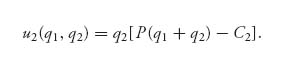
From firm 1’s perspective this is a random variable because of the unknown cost. The way to find an equilibrium now is the following:
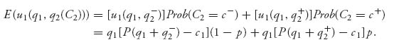
For example, let’s take the price function P(q) = Γ −q, 0 ≤ q ≤ Γ:
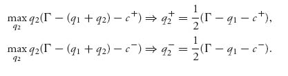
1. Firm 2 has the cost of production c+ q2 with probability p and the cost of production c−q2 with probability 1−p. Firm 2 will solve the problem for each cost c+, c− assuming that q1 is known:
2. Next, firm 1 will maximize the expected profit using the two quantities q2+, q2−. Firm 1 seeks the production quantity q1, which solves
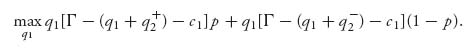
This is maximized at
3. Summarizing, we now have the following system of equations for the variables q1, q2−, q2+:
Observe that q1 is the expected quantity of production assuming that firm 2 produces q2+ with probability p and q2− with probability 1 − p.
Solving the equations in (3), we finally arrive at the optimal production levels:
Note that if we require that the production levels be nonnegative, we need to put some conditions on the costs and Γ.
5.2.4 THE BERTRAND MODEL
Joseph Bertrand16 didn’t like Cournot’s model. He thought firms should set prices to accommodate demand, not production quantities. Here is the setup he introduced. We again have two companies making identical gadgets. In this model, they can set prices, not quantities, and they will only produce the quantity demanded at the given price. So the quantity sold is a function of the price set by each firm, say, q = Γ −p. This is better referred to as the demand function for a given price:
![]()
In the classic problem, the model says that if both firms charge the same price, they will split the market evenly, with each selling exactly half of the total sold. The company that charges a lower price will capture the entire market. We have to assume that each company has enough capacity to make the entire quantity demanded if it captures the whole market. The cost to make gadgets is still ci, i = 1, 2, dollars per unit gadget. We first assume the firms have differing costs:
![]()
The profit function for firm i = 1, 2, assuming that firm 1 sets the price as p1 and firm 2 sets the price at p2, is
This says that if firm 1 sets the price lower than firm 2, firm 1’s profit will be (price- cost)× quantity demanded; if the prices are the same, firm 1’s profits will be (![]() ) (price-cost)× quantity demanded; and zero if firm 1’s price of a gadget is greater than firm 2’s. This assumes that the lower price captures the entire market. Similarly, firm 2’s profit function is
) (price-cost)× quantity demanded; and zero if firm 1’s price of a gadget is greater than firm 2’s. This assumes that the lower price captures the entire market. Similarly, firm 2’s profit function is
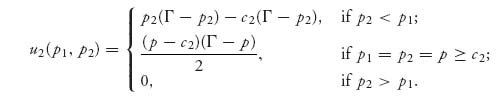
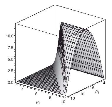
Figure 5.5 is a plot of u1(p1, p2) with Γ = 10, c1 = 3.
FIGURE 5.5 Discontinuous payoff function for firm 1.
Now we have to find a Nash equilibrium for these discontinuous (nondifferentiable) payoff functions. Let’s suppose that there is a Nash equilibrium point at (p1*, p2*). By definition, we have
![]()
Let’s break this down by considering three cases:
Case 1. p1* > p2*. Then it should be true that firm 2, having a lower price, captures the entire market so that for firm 1
![]()
But if we take any price c1 < p1 < p2*, the right side will be
![]()
so p1* > p2* cannot hold and still have (p1*, p2*) a Nash equilibrium.
Case 2. p1* < p2*. Then it should be true that firm 1 captures the entire market and so for firm 2
![]()
But if we take any price for firm 2 with c2 < p2 < p1*, the right side will be
![]()
that is, strictly positive, and again it cannot be that p1* < p2* and fulfill the requirements of a Nash equilibrium. So the only case left is the following.
Case 3. p1* = p2*. But then the two firms split the market and we must have for firm 1
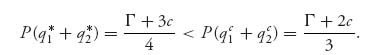
If we take firm 1’s price to be p1 = p1* −ε < p2* with really small ε > 0, then firm 1 drops the price ever so slightly below firm 2’s price. Under the Bertrand model, firm 1 will capture the entire market at price p1 so that in this case we have

This inequality won’t be true for every ε, but it will be true for small enough ε > 0, (say, 0 < ε < ![]() ).
).
Thus, in all cases, we can find prices so that the condition that (p1*, p2*) be a Nash point is violated and so there is no Nash equilibrium in pure strategies. But there is one case when there is a Nash equilibrium. In the above analysis, we assumed in several places that prices would have to be above costs. What if we drop that assumption? The first thing that happens is that in case 3 we won’t be able to find a positive ε to drop p1*.
What’s the problem here? It is that neither player has a continuous profit function (as you can see in Figure 5.5). By lowering the price just below the competitor’s price, the firm with the lower price can capture the entire market. So the incentive is to continue lowering the price of a gadget. In fact, we are led to believe that maybe p1* = c1, p2* = c2 is a Nash equilibrium. Let’s check that, and let’s just assume that c1 < c2, because a similar argument would apply if c1 > c2.
In this case, u1(c1, c2) = 0, and if this is a Nash equilibrium, then it must be true that u1(c1, c2) = 0 ≥ u1(p1, c2) for all p1. But if we take any price c1 < p1 < c2, then
![]()
and we conclude that (c1, c2) also is not a Nash equilibrium. The only way that this could work is if c1 = c2 = c, so the costs to each firm are the same. In this case, we leave it as an exercise to show that p1* = c, p2* = c is a Nash equilibrium and optimal profits are zero for each firm. So, what good is this if the firms make no money, and even that is true only when their costs are the same? This leads us to examine assumptions about exactly how profits arise in competing firms. Is it strictly prices and costs, or are there other factors involved?
The Traveler’s Paradox Example 5.9 illustrates what goes wrong with the Bertrand model. It also shows that when there is an incentive to drop to the lowest price, it leads to unrealistic expectations. On the other hand, the Bertrand model can be modified to take other factors into account like demand sensitivities to prices or production quantity capacity limits. These modifications are explored in the exercises.
5.2.5 THE STACKELBERG MODEL
What happens if two competing firms don’t choose the production quantities at the same time, but choose sequentially one after the other? Stackelberg17 gave an answer to this question. In this model, we will assume that there is a dominant firm, say, firm 1, who will announce its production quantity publicly. Then firm 2 will decide how much to produce. In other words, given that one firm knows the production quantity of the other, determine how much each will or should produce.
Suppose that firm 1 announces that it will produce q1 gadgets at cost c1 dollars per unit. It is then up to firm 2 to decide how many gadgets, say, q2 at cost c2, it will produce. We again assume that the unit costs are constant. The price per unit will then be considered a function of the total quantity produced so that p = p(q1, q2) = (Γ −q1−q2)+ = max { Γ −q1−q2, 0}. The profit functions will be
These are the same as in the simplest Cournot model, but now q1 is fixed as given. It is not variable when firm 1 announces it. So what we are really looking for is the best response of firm 2 to the production announcement q1 by firm 1. In other words, firm 2 wants to know how to choose q2 = q2(q1) so as to
![]()
This is given by calculus as
This is the amount that firm 2 should produce when firm 1 announces the quantity of production q1. It is the same best response function for firm 2 as in the Cournot model.
Now, firm 1 has some clever employees who know calculus and game theory and can perform this calculation as well as we can. Firm 1 knows what firm 2’s optimal production quantity should be, given its own announcement of q1. Therefore, firm 1 should choose q1 to maximize its own profit function knowing that firm 2 will use production quantity q2(q1):
Firm 1 wants to choose q1 to make this as large as possible. By calculus, we find that
The optimal production quantity for firm 2 is
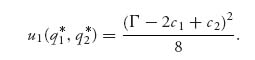
The equilibrium profit function for firm 2 is then
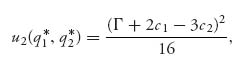
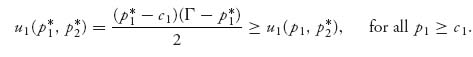
and for firm 1, it is
For comparison, we will set c1 = c2 = c and then recall the optimal production quantities for the Cournot model:
The equilibrium profit functions were
In the Stackelberg model, we have
So firm 1 produces more and firm 2 produces less in the Stackelberg model than if firm 2 did not have the information announced by firm 1. For the firm’s profits, we have
Firm 1 makes more money by announcing the production level, and firm 2 makes less with the information.
One last comparison is the total quantity produced
and the price at equilibrium (recall that Γ > c):
5.2.6 ENTRY DETERRENCE
In this example, we ask the following question. If there is currently only one firm producing a gadget, what should be the price of the gadget in order to make it unprofitable for another firm to enter the market and compete with firm 1? This is a famous problem in economics called the entry deterrence problem.
Of course, a monopolist may charge any price at all as long as there is a demand for gadgets at that price. But it should also be true that competition should lower prices, implying that the price to prevent entry by a competitor should be lower than what the firm would otherwise set.
We call the existing company firm 1 and the potential challenger firm 2. The demand function is p = D(q) = (Γ −q)+.
Now, before the challenger enters the market the profit function to firm 1 is
![]()
where we assume that the cost function C(q) = aq + b, with Γ > a, b > 0. This cost function includes a fixed cost of b > 0 because even if the firm produces nothing, it still has expenses.
Now firm 1 is acting as a monopolist in our model because it has no competition. So firm 1 wants to maximize profit, which gives a production quantity of
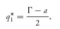
and maximum profit for a monopolist of
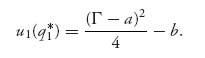
In addition, the price of a gadget at this quantity of production will be
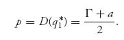
Now firm 2 enters the picture and calculates firm 2’s profit function knowing that firm 1 will or should produce q1* = (Γ −a)/2 to get firm 2’s payoff function:
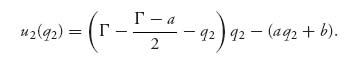
So firm 2 calculates its maximum possible profit and optimal production quantity as
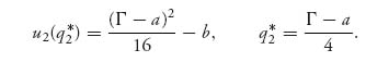
The price of gadgets will now drop (recall Γ > a) to
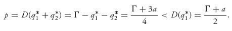
As long as u2(q2*) ≥ 0, firm 2 has an incentive to enter the market. If we interpret the constant b as a fixed cost to enter the market, this will require that
or else firm 2 cannot make a profit.
Now here is a more serious analysis because firm 1 is not about to sit by idly and let another firm enter the market. Therefore, firm 1 will now analyze the Cournot model assuming that there is a firm 2 against which firm 1 is competing. Firm 1 looks at the profit function for firm 2:
![]()
and maximizes this as a function of q2 to get
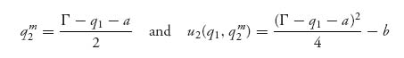
as the maximum profit to firm 2 if firm 1 produces q1 gadgets. Firm 1 reasons that it can set q1 so that firm 2’s profit is zero:
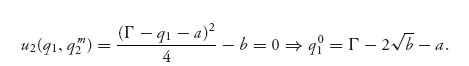
This gives a zero profit to firm 2. Consequently, if firm 1 decides to produce q10 gadgets, firm 2 has no incentive to enter the market. The price at this quantity will be
![]()
and the profit for firm 1 at this level of production will be
![]()
This puts a requirement on Γ that Γ > a + ![]() , or else firm 1 will also make a zero profit.
, or else firm 1 will also make a zero profit.
Problems
5.26 In the Cournot model, we assumed there were two firms in competition. Instead suppose that there is only one firm, a monopolist, producing at quantity q. Formulate a model to determine the optimal production quantity. Compare the optimal production quantity for the monopolist with the quantities derived in the Cournot duopoly assuming c1 = c2 = c. Does competition produce lower prices?
5.27 The Cournot model assumed the firms acted independently. Suppose instead the two firms collude to set production quantities.
5.28 Two firms produce identical widgets. The price function is P(q) = (150−q)+ and the cost to produce q widgets is C(q) = 120 q − ![]() q2 for each firm.
q2 for each firm.
5.29 Suppose instead of two firms in the Cournot model with payoff functions (5.1), that there are N firms. Formulate this model and find the optimal quantities each of the N firms should produce. Instead of a duopoly, this is an oligopoly. What happens when the firms all have the same costs and N → ∞?
5.30 Two firms produce identical products. The market price for total production quantity q is P(q) = 100 − 2 ![]() . Firm 1’s production cost is C1(q1) = q1 + 10, and firm 2’s production cost is C2(q2) = 2q2 + 5. Find the profit functions and the Nash equilibrium quantities of production and profits.
. Firm 1’s production cost is C1(q1) = q1 + 10, and firm 2’s production cost is C2(q2) = 2q2 + 5. Find the profit functions and the Nash equilibrium quantities of production and profits.
5.31 Consider the Cournot duopoly model with a somewhat more realistic price function given by
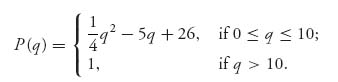
Take the cost of producing a gadget at c = 1 for both firms.
5.32 Compare profits for firm 1 in the model with uncertain costs and the standard Cournot model. Assume Γ = 15, c1 = 4, c+ = 5, c− = 1 and p = 0.5.
5.33 Suppose that we consider the Cournot model with uncertain costs but with three possible costs for firm 2, Prob(C2 = ci) = pi, i = 1, 2, 3, where pi ≥ 0, p1 + p2 + p3 = 1.
5.34 Suppose that two firms have constant unit costs c1 = 2, c2 = 1, and Γ = 19 in the Stackelberg model.
5.35 Set up and solve a Stackelberg model given three firms with constant unit costs c1, c2, c3 and firm 1 announcing production quantity q1.
5.36 Gadget prices range in the interval (0, 100]. Assume the demand function is simply D(p) = 100−p. If two firms make the gadget, firm 1’s profit function is given by
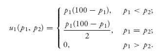
5.37 In the Bertrand model of this section, show that if c1 = c2 = c, then (p1*, p2*) = (c, c) is a Nash equilibrium but each firm makes zero profit.
5.38 Determine the entry deterrence level of production for the model in this section for firm 1 given Γ = 100, a = 2, b = 10.
5.39 We could make one more adjustment in the Bertrand model of this section and see what effect it has on the model. What if we put a limit on the total quantity that a firm can produce? This limits the supply and possibly will put a floor on prices. Let K ≥ ![]() k denote the maximum quantity of gadgets that each firm can produce and recall that D(p) = Γ −p is the quantity of gadgets demanded at price p. Find the profit functions for each firm.
k denote the maximum quantity of gadgets that each firm can produce and recall that D(p) = Γ −p is the quantity of gadgets demanded at price p. Find the profit functions for each firm.
5.40 Suppose that the demand functions in the Bertrand model are given by
![]()
where 1 ≥ b > 0. This says that the quantity of gadgets sold by a firm will increase if the price set by the opposing firm is too high. Assume that both firms have a cost of production c ≤ min { p1, p2}. Then, since profit is revenue minus costs the profit functions will be given by
![]()
and
![]()
Find a Nash equilibrium and the profits at equilibrium.
5.41 Suppose that firm 1 announces a price in the Bertrand model with demand functions
![]()
where 1 ≥ b > 0. Assume the firms have unit costs of production c1, c2.
Construct the Stackelberg model; firm 2 should find the best response p2 = p2 (p1) to maximize u2(p1, p2) and then firm 1 should choose p1 to maximize u1(p1, p2(p1)). Find the equilibrium prices and profits. What is the result when Γ = 100, c1 = 5, c2 = 1, b = 1/2?