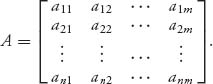
A matrix is a rectangular collection of numbers. If there are n rows and m columns, we write the matrix as An × m, and the numbers of the matrix are aij, where i gives the row number and j gives the column number. These are also called the dimensions of the matrix. We compactly write 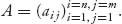 In rectangular form
1. We add two matrices that have the same dimensions, A + B, by adding the respective components A + B = (aij + bij), or

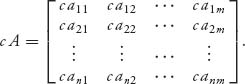
2. A matrix may be multiplied by a scalar c by multiplying every element of A by c; that is, c A = (c aij) or
3. We may multiply two matrices An×m and Bm × k only if the number of columns of A is exactly the same as the number of rows of B. You have to be careful because not only is A · B ≠ B · A; in general, it is not even defined if the rows and columns don’t match up. So, if A = An × m and B = Bm × k, then C = A · B is defined and C = Cn × k, and is given by
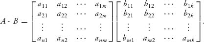
We multiply each row i = 1, 2, …, n of A by each column j = 1, 2, …, k of B in this way:
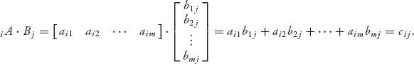
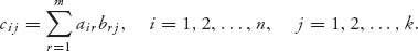
This gives the (i, j)th element of the matrix C. The matrix Cn × k = (cij) has elements written compactly as
4. As special cases of multiplication that we use throughout this book
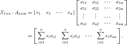
Each element of the result is E(X, j), j = 1, 2, ···, m.
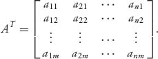
5. If we have any matrix An × m, the transpose of A is written as AT and is the m × n matrix, which is A with the rows and columns switched:
If Y1 × m is a row matrix, then YT is an m × 1 column matrix, so we may multiply An × m by YT on the right to get
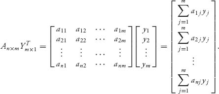
Each element of the result is E(i, Y), i = 1, 2, …, n.
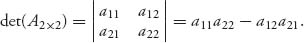
6. A square matrix An × n has an inverse A-1 if there is a matrix Bn × n that satisfies A · B = B · A = I, and then B is written as A-1. Finding the inverse is computationally tough, but luckily you can determine whether there is an inverse by finding the determinant of A. The linear algebra theorem says that A-1 exists if and only if det(A) ≠ 0. The determinant of a 2 × 2 matrix is easy to calculate by hand:
One way to calculate the determinant of a larger matrix is expansion by minors which we illustrate for a 3 × 3 matrix:
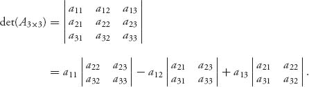
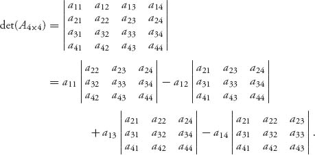
This reduces the calculation of the determinant of a 3 × 3 matrix to the calculation of the determinants of three 2 × 2 matrices, which are called the minors of A. They are obtained by crossing out the row and column of the element in the first row (other rows may also be used). The determinant of the minor is multiplied by the element and the sign + or − alternates starting with a + for the first element. Here is the determinant for a 4 × 4 reduced to four 3 × 3 determinants:
7. A system of linear equations for the unknowns
may be written in matrix form as

where
This is called an
inhomogeneous system if

and a
homogeneous system if

If
A is a square matrix and is invertible, then

is the one and only solution. In particular, if

then

is the only solution.
8. A matrix An × m has associated with it a number called the rank of A, which is the largest square submatrix of A that has a nonzero determinant. So, if A is a 4 × 4 invertible matrix, then rank(A) = 4. Another way to calculate the rank of A is to row-reduce the matrix to row-reduced echelon form. The number of nonzero rows is rank(A).
9. The rank of a matrix is intimately connected to the solution of equations An × m ym × 1 = bn × 1. This system will have a unique solution if and only if rank(A) = m. If rank(A)< m, then Aym × 1 = bn × 1 has an infinite number of solutions. For the homogeneous system Aym × 1 = 0n × 1, this has a unique solution, namely, ym × 1 = 0m × 1, if and only if rank(A) = m. In any other case, Aym × 1 = 0n × 1 has an infinite number of solutions.
To simplify notation we will drop the superscript T for the transpose of a single row matrix.