CHAPTER 5
Comparing More Than Two Related Samples: The Friedman Test
5.1 Objectives
In this chapter, you will learn the following items:
- How to compute the Friedman test.
- How to perform contrasts to compare samples.
- How to perform the Friedman test and associated sample contrasts using SPSS®.
5.2 Introduction
Most public school divisions take pride in the percentage of their graduates admitted to college. A large school division might want to determine if these college admission rates are changing or stagnant. The division could compare the percentages of graduates admitted to college from each of its 10 high schools over the past 5 years. Each year would constitute a group, or sample, of percentages from each school. In other words, the study would include five groups, and each group would include 10 values.
The samples in the example are dependent, or related, since each school has a percentage for each year. The Friedman test is a nonparametric statistical procedure for comparing more than two samples that are related. The parametric equivalent to this test is the repeated measures analysis of variance (ANOVA).
When the Friedman test leads to significant results, then at least one of the samples is different from the other samples. However, the Friedman test does not identify where the difference(s) occur. Moreover, it does not identify how many differences occur. In order to identify the particular differences between sample pairs, a researcher might use sample contrasts, or post hoc tests, to analyze the specific sample pairs for significant difference(s). The Wilcoxon signed rank test (see Chapter 3) is a useful method for performing sample contrasts between related sample sets.
In this chapter, we will describe how to perform and interpret a Friedman test followed with sample contrasts. We will also explain how to perform the procedures using SPSS. Finally, we offer varied examples of these nonparametric statistics from the literature.
5.3 Computing the Friedman Test Statistic
The Friedman test is used to compare more than two dependent samples. When stating our hypotheses, we state them in terms of the population. Moreover, we examine the population medians, θi, when performing the Friedman test.
To compute the Friedman test statistic Fr, we begin by creating a table of our data. List the research subjects to create the rows. Place the values for each condition in columns next to the appropriate subjects. Then, rank the values for each subject across each condition. If there are no ties from the ranks, use Formula 5.1 to determine the Friedman test statistic Fr:
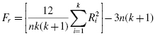
where n is the number of rows, or subjects, k is the number of columns, or conditions, and Ri is the sum of the ranks from column, or condition, i.
If ranking of values results in any ties, use Formula 5.2 to determine the Friedman test statistic Fr:
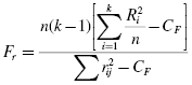
where n is the number of rows, or subjects, k is the number of columns, or conditions, Ri is the sum of the ranks from column, or condition, i, CF is the ties correction, ![]() , and rij is the rank corresponding to subject j in column i.
, and rij is the rank corresponding to subject j in column i.
The degrees of freedom for the Friedman test is determined by using Formula 5.3:
Where df is the degrees of freedom and k is the number of groups.
Once the test statistic Fr is computed, it can be compared with a table of critical values (see Table B.5 in Appendix B) to examine the groups for significant differences. However, if the number of groups, k, or the number of values in a group, n, exceeds those available from the table, then a large sample approximation may be performed. Use a table with the χ2 distribution (see Table B.2 in Appendix B) to obtain a critical value when performing a large sample approximation.
If the Fr statistic is not significant, then no differences exist between any of the related conditions. However, if the Fr statistic is significant, then a difference exists between at least two of the conditions. Therefore, a researcher might use sample contrasts between individual pairs of conditions, or post hoc tests, to determine which of the condition pairs are significantly different.
When performing multiple sample contrasts, the type I error rate tends to become inflated. Therefore, the initial level of risk, or α, must be adjusted. We demonstrate the Bonferroni procedure, shown in Formula 5.4, to adjust α:
where αB is the adjusted level of risk, α is the original level of risk, and k is the number of comparisons.
5.3.1 Sample Friedman's Test (Small Data Samples without Ties)
A manager is struggling with the chronic tardiness of her seven employees. She tries two strategies to improve employee timeliness. First, over the course of a month, she punishes employees with a $10 paycheck deduction for each day that they arrive late. Second, the following month, she punishes employees by docking their pay $20 for each day that they do not arrive on time.
Table 5.1 shows the number of times each employee was late in a given month. The baseline shows the employees' monthly tardiness before the strategies. Month 1 shows the employees' monthly tardiness after a month of the $10 paycheck deductions. Month 2 shows the employees' monthly tardiness after a month of the $20 paycheck deductions.
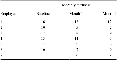
We want to determine if either of the paycheck deduction strategies reduced employee tardiness. Since the sample sizes are small (n < 20), we require a nonparametric test. The Friedman test is the best statistic to analyze the data and test the hypothesis.
5.3.1.1 State the Null and Research Hypotheses
The null hypothesis states that neither of the manager's strategies will change employee tardiness. The research hypothesis states that one or both of the manager's strategies will reduce employee tardiness.
The null hypothesis is
HO: θB = θM1 = θM2
The research hypothesis is
HA: One or both of the manager's strategies will reduce employee tardiness.
5.3.1.2 Set the Level of Risk (or the Level of Significance) Associated with the Null Hypothesis
The level of risk, also called an alpha (α), is frequently set at 0.05. We will use α = 0.05 in our example. In other words, there is a 95% chance that any observed statistical difference will be real and not due to chance.
5.3.1.3 Choose the Appropriate Test Statistic
The data are obtained from three dependent, or related, conditions that report employees' number of monthly tardiness. The three samples are small with some violations of our assumptions of normality. Since we are comparing three dependent conditions, we will use the Friedman test.
5.3.1.4 Compute the Test Statistic
First, rank the values from each employee, or subject (see Table 5.2).
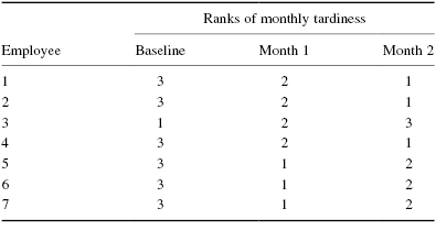
Next, compute the sum of ranks for each condition. The ranks in each group are added to obtain a total R-value for the group.
For the baseline condition,
For month 1,
For month 2,
These R-values are used to compute the Fr test statistic. Use Formula 5.1 since there were no ties involved in the ranking:
5.3.1.5 Determine the Value Needed for Rejection of the Null Hypothesis Using the Appropriate Table of Critical Values for the Particular Statistic
We will use the critical value table for the Friedman test (see Table B.5 in Appendix B) since it includes the number of groups, k, and the number of samples, n, for our data. In this case, we look for the critical value for k = 3 and n = 7 with α = 0.05. Table B.5 returns a critical value for the Friedman test of 7.14.
5.3.1.6 Compare the Obtained Value with the Critical Value
The critical value for rejecting the null hypothesis is 7.14 and the obtained value is Fr = 5.429. If the critical value is less than or equal to the obtained value, we must reject the null hypothesis. If instead, the critical value exceeds the obtained value, we do not reject the null hypothesis. Since the critical value exceeds the obtained value, we do not reject the null hypothesis.
5.3.1.7 Interpret the Results
We did not reject the null hypothesis, suggesting that no significant difference exists between any of the three conditions. Therefore, no further comparisons are necessary with these data.
5.3.1.8 Reporting the Results
The reporting of results for the Friedman test should include such information as the number of subjects, the Fr statistic, degrees of freedom, and p-value's relation to α.
For this example, the frequencies of employees' (n = 7) tardiness were compared over three conditions. The Friedman test was not significant (Fr(2) = 5.429, p > 0.05). Therefore, we can state that the data do not support punishing tardy employees with $10 or $20 paycheck deductions.
5.3.2 Sample Friedman's Test (Small Data Samples with Ties)
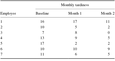
After the manager's failure to reduce employee tardiness with paycheck deductions, she decided to try a different approach. This time, she rewarded employees when they arrived to work on-time. Again, she tries two strategies to improve employee timeliness. First, over the course of a month, she rewards employees with a $10 bonus for each day that they arrive on-time. Second, the following month, she rewards employees with a $20 bonus for each day that they arrive on-time.
Table 5.3 shows the number of times each employee was late in a given month. The baseline shows the employees' monthly tardiness before any of the strategies in either example. Month 1 shows the employees' monthly tardiness after a month of the $10 bonuses. Month 2 shows the employees' monthly tardiness after a month of the $20 bonuses.
We want to determine if either of the strategies reduced employee tardiness. Again, since the sample sizes are small (n < 20), we use a nonparametric test. The Friedman test is a good statistic to analyze the data and test the hypothesis.
5.3.2.1 State the Null and Research Hypotheses
The null hypothesis states that neither of the manager's strategies will change employee tardiness. The research hypothesis states that one or both of the manager's strategies will reduce employee tardiness.
The null hypothesis is
HO: θB = θM1 = θM2
The research hypothesis is
HA: One or both of the manager's strategies will reduce employee tardiness.
5.3.2.2 Set the Level of Risk (or the Level of Significance) Associated with the Null Hypothesis
The level of risk, also called an alpha (α), is frequently set at 0.05. We will use α = 0.05 in our example. In other words, there is a 95% chance that any observed statistical difference will be real and not due to chance.
5.3.2.3 Choose the Appropriate Test Statistic
The data are obtained from three dependent, or related, conditions that report employees' number of monthly tardiness. The three samples are small with some violations of our assumptions of normality. Since we are comparing three dependent conditions, we will use the Friedman test.
5.3.2.4 Compute the Test Statistic
First, rank the values from each employee, or subject (see Table 5.4).
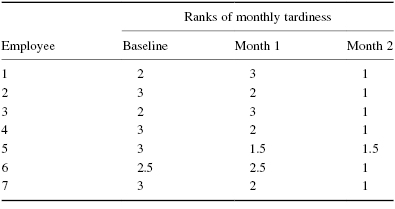
Next, compute the sum of ranks for each condition. The ranks in each group are added to obtain a total R-value for the group.
For the baseline condition,
For month 1,
For month 2,
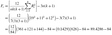
These R-values are used to compute the Fr test statistic. Since there were ties involved in the rankings, we must use Formula 5.2. Finding the values for CF and ![]() first will simplify the calculation:
first will simplify the calculation:
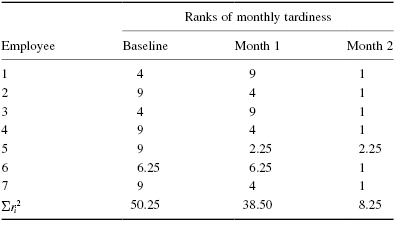
To find ![]() , square all of the ranks. Then, add all of the squared ranks together (see Table 5.5):
, square all of the ranks. Then, add all of the squared ranks together (see Table 5.5):
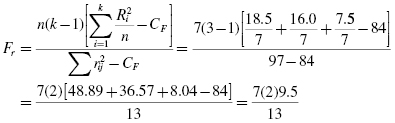
Now that we have CF and ![]() , we are ready for Formula 5.2:
, we are ready for Formula 5.2:
5.3.2.5 Determine the Value Needed for Rejection of the Null Hypothesis Using the Appropriate Table of Critical Values for the Particular Statistic
We will use the critical value table for the Friedman test (see Table B.5 in Appendix B) since it includes the number of groups, k, and the number of samples, n, for our data. In this case, we look for the critical value for k = 3 and n = 7 with α = 0.05. Table B.5 returns a critical value for the Friedman test of 7.14.
5.3.2.6 Compare the Obtained Value with the Critical Value
The critical value for rejecting the null hypothesis is 7.14 and the obtained value is Fr = 10.23. If the critical value is less than or equal to the obtained value, we must reject the null hypothesis. If instead, the critical value exceeds the obtained value, we do not reject the null hypothesis. Since the obtained value exceeds the critical value, we reject the null hypothesis.
5.3.2.7 Interpret the Results
We rejected the null hypothesis, suggesting that a significant difference exists between one or more of the three conditions. In particular, both strategies seemed to result in less tardiness among employees. However, describing specific differences in this manner is speculative. Therefore, we need a technique for statistically identifying difference between conditions, or contrasts.
Sample Contrasts, or Post Hoc Tests
The Friedman test identifies if a statistical difference exists; however, it does not identify how many differences exist and which conditions are different. To identify which conditions are different and which are not, we use a procedure called contrasts or post hoc tests. An appropriate test to use when comparing two related samples at a time is the Wilcoxon signed rank test described in Chapter 3.
It is important to note that performing several two-sample tests has a tendency to inflate the type I error rate. In our example, we would compare three groups, k = 3. At an α = 0.05, the type I error rate would equal 1 − (1 − 0.05)3 = 0.14.
To compensate for this error inflation, we demonstrate the Bonferroni procedure (see Formula 5.4). With this technique, we use a corrected α with the Wilcoxon signed rank tests to determine significant differences between conditions. For our example, we are only comparing month 1 and month 2 against the baseline. We are not comparing month 1 against month 2. Therefore, we are only making two comparisons and k = 2:
When we compare the three samples with the Wilcoxon signed rank tests using αB, we obtain the results presented in Table 5.6. Notice that the significance is one-tailed, or directional, since we were seeking a decline in tardiness.
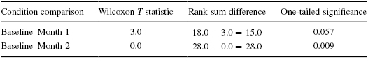
Using αB = 0.025, we notice that the baseline–month 1 comparison does not demonstrate a significant difference (p > 0.025). However, the baseline–month 2 comparison does demonstrate a significant difference (p < 0.025). Therefore, the data indicate that the $20 bonus reduces tardiness while the $10 bonus does not.
Note that if you are not comparing all of the samples for the Friedman test, then k is only the number of comparisons you are making with the Wilcoxon signed rank tests. Therefore, comparing fewer samples will increase the chances of finding a significant difference.
5.3.2.8 Reporting the Results
The reporting of results for the Friedman test should include such information as the number of subjects, the Fr statistic, degrees of freedom, and p-value's relation to α.
For this example, the frequencies of employees' (n = 7) tardiness were compared over three conditions. The Friedman test was significant (Fr(2) = 10.23, p < 0.05). In addition, follow-up contrasts using Wilcoxon signed rank tests revealed that $20 bonus reduces tardiness, while the $10 bonus does not.
5.3.3 Performing the Friedman Test Using SPSS
We will analyze the data from the example earlier using SPSS.
5.3.3.1 Define Your Variables
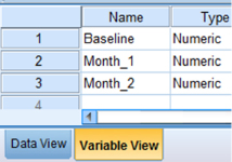
First, click the “Variable View” tab at the bottom of your screen. Then, type the names of your variables in the “Name” column. As shown in Figure 5.1, we have named our variables “Baseline,” “Month_1,” and “Month_2.”
5.3.3.2 Type in Your Values
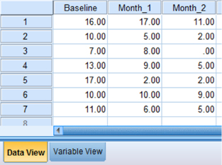
Click the “Data View” tab at the bottom of your screen and type your data under the variable names. As shown in Figure 5.2, we are comparing “Baseline,” “Month_1,” and “Month_2.”
5.3.3.3 Analyze Your Data
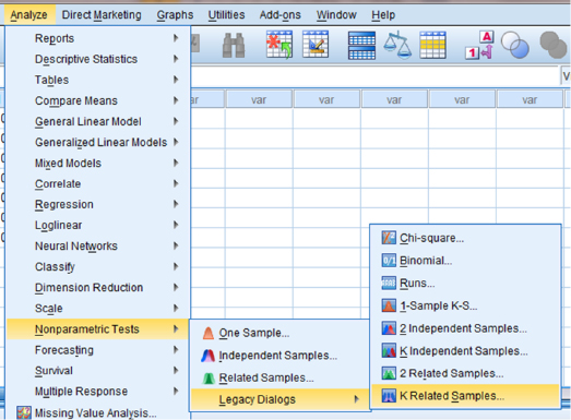
As shown in Figure 5.3, use the pull-down menus to choose “Analyze,” “Nonparametric Tests,” “Legacy Dialogs,” and “K Related Samples… .”
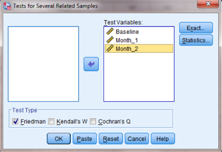
Select each of the variables that you want to compare and click the button in the middle to move it to the “Test Variables:” box as shown in Figure 5.4. Notice that the “Friedman” box is checked by default. After the variables are in the “Test Variables:” box, click “OK” to perform the analysis.
5.3.3.4 Interpret the Results from the SPSS Output Window
The first output table in SPSS Output 5.1 provides the mean ranks of each condition. The second output table provides the Friedman test statistic, 10.231. Since this test uses a χ2 distribution, SPSS calls the Fr statistic “Chi-Square.” This table also returns the number of subjects (n = 7) degrees of freedom (df = 2) and the significance (p = 0.006).
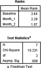
Based on the results from SPSS, three conditions were compared among employees (n = 7). The Friedman test was significant (Fr(2) = 10.23, p < 0.05). In order to compare individual pairs of conditions, contrasts may be used.
Note that to perform Wilcoxon signed rank tests for sample contrasts, remember to use your corrected level of risk, αB, when examining your significance.
5.3.4 Sample Friedman's Test (Large Data Samples without Ties)
After hearing of the manager's success, the head office transferred her to a larger branch office. The transfer was strategic because this larger branch is dealing with tardiness issues among employees. The manager suggests that she use the same successful incentives for employee timeliness. Due to financial limitations, however, she is limited to offering employees smaller bonuses. First, over the course of a month, she rewards employees with a $2 bonus for each day that they arrive on-time. Second, the following month, she rewards employees with a $5 bonus for each day that they arrive on-time.
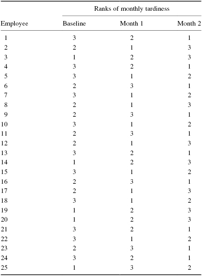
Table 5.7 shows the number of times each employee was late in a given month. The baseline shows the employees' monthly tardiness before any of the strategies in either example. Month 1 shows the employees' monthly tardiness after a month with $2 bonuses. Month 2 shows the employees' monthly tardiness after a month with $5 bonuses.
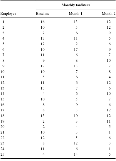
We want to determine if either of the paycheck bonus strategies reduced employee tardiness. Since the sample sizes are large (n > 20), we will use χ2 for the critical value. The Friedman test is a good statistic to analyze the data and test the hypothesis.
5.3.4.1 State the Null and Research Hypotheses
The null hypothesis states that neither of the manager's strategies will change employee tardiness. The research hypothesis states that one or both of the manager's strategies will reduce employee tardiness.
The null hypothesis is
HO: θB = θM1 = θM2
The research hypothesis is
HA: One or both of the manager's strategies will reduce employee tardiness.
5.3.4.2 Set the Level of Risk (or the Level of Significance) Associated with the Null Hypothesis
The level of risk, also called an alpha (α), is frequently set at 0.05. We will use α = 0.05 in our example. In other words, there is a 95% chance that any observed statistical difference will be real and not due to chance.
5.3.4.3 Choose the Appropriate Test Statistic
The data are obtained from three dependent, or related, conditions that report employees' number of monthly tardiness. Since we are comparing three dependent conditions, we will use the Friedman test.
5.3.4.4 Compute the Test Statistic
First, rank the values from each employee or subject (see Table 5.8).
Next, compute the sum of ranks for each condition. The ranks in each group are added to obtain a total R-value for the group.
For the baseline condition,
For month 1,
For month 2,
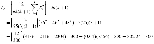
These R-values are used to compute the Fr test statistic. Use Formula 5.1 since there were no ties involved in the ranking:
5.3.4.5 Determine the Value Needed for Rejection of the Null Hypothesis Using the Appropriate Table of Critical Values for the Particular Statistic
Since the data are a large sample, we will use the χ2 distribution (see Table B.2 found in Appendix B) to find the critical value for the Friedman test. In this case, we look for the critical value for df = 2 and α = 0.05. Using the table, the critical value for rejecting the null hypothesis is 5.99.
5.3.4.6 Compare the Obtained Value with the Critical Value
The critical value for rejecting the null hypothesis is 5.99 and the obtained value is Fr = 2.24. If the critical value is less than or equal to the obtained value, we must reject the null hypothesis. If instead, the critical value exceeds the obtained value, we do not reject the null hypothesis. Since the critical value exceeds the obtained value, we do not reject the null hypothesis.
5.3.4.7 Interpret the Results
We did not reject the null hypothesis, suggesting that no significant difference exists between one or more of the three conditions. In particular, the data suggest that neither strategy seemed to result in less tardiness among employees.
5.3.4.8 Reporting the Results
The reporting of results for the Friedman test should include such information as the number of subjects, the Fr statistic, degrees of freedom, and p-value's relation to α. For this example, the frequencies of employees' (n = 25) tardiness were compared over three conditions. The Friedman test was not significant (Fr(2) = 2.24, p > 0.05). Therefore, we can state that the data do not support providing employees with the $2 or $5 paycheck incentive.
5.4 Examples from the Literature
Varied examples of the nonparametric procedures described in this chapter are to be shown later. We have summarized each study's research problem and researchers' rationale(s) for choosing a nonparametric approach. We encourage you to obtain these studies if you are interested in their results.
Marston (1996) examined teachers' attitudes toward three models for servicing elementary students with mild disabilities. He compared special education resource teachers' ratings of the three models (inclusion only, combined services, and pull-out only) using a Friedman test. He chose this nonparametric test because the teachers' attitude responses were based on rankings. When the Friedman test produced significant results, he modified the α with the Bonferroni procedure in order to avoid a ballooned type I error rate with follow-up comparisons.
From a Russian high school's English as a foreign language program, Savignon and Sysoyev (2002) examined 30 students' responses to explicit training in coping strategies for particular social and cultural situations. Since the researchers considered each student a block in a randomized block study, they used a Friedman test to compare the 30 students, or groups. A nonparametric test was chosen because there were only two possible responses for each strategy (1 = strategy was difficult; 0 = strategy was not difficult). When the Friedman test produced significant results, they used a follow-up sign test to examine each pair for differences in response to find out which of seven strategies were more difficult than others.
Cady et al. (2006) examined math teachers beliefs about the teaching and learning of mathematics over time. Since their sample size was small (n = 12), they used a Friedman test to compare scores of participants' survey responses. When participants' scores on the surveys differed significantly, the researchers performed follow-up pairwise analyses with the Wilcoxon signed rank test.
Hardré et al. (2007) sought to determine if computer-based, paper-based, and web-based test administrations produce the same results. They compared university students' performance on each of the three test styles. Since normality violations were observed, the researchers used a Friedman test to compare correlations of the three methods. Follow-up contrast tests were not performed since no significant differences were observed.
5.5 Summary
More than two samples that are related may be compared using the Friedman test. The parametric equivalent to this test is known as the repeated measures ANOVA. When the Friedman test produces significant results, it does not identify which nor how many pairs of conditions are significantly different. The Wilcoxon signed rank test, with a Bonferroni procedure to avoid type I error rate inflation, is a useful method for comparing individual condition pairs.
In this chapter, we described how to perform and interpret a Friedman test followed with sample contrasts. We also explained how to perform the procedures using SPSS. Finally, we offered varied examples of these nonparametric statistics from the literature. The next chapter will involve a nonparametric procedure for comparing more than two unrelated samples.
5.6 Practice Questions
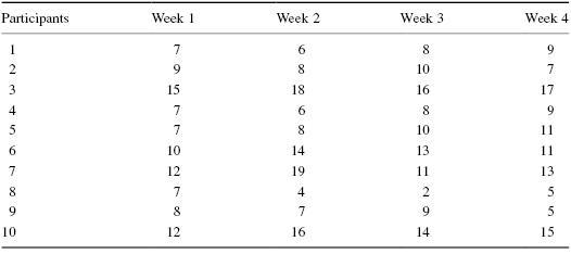
1. A graduate student performed a pilot study for his dissertation. He wanted to examine the effects of animal companionship on elderly males. He selected 10 male participants from a nursing home. Then he used an ABAB research design, where A represented a week with the absence of a cat and B represented a week with the presence of a cat. At the end of each week, he administered a 20-point survey to measure quality of life satisfaction. The survey results are presented in Table 5.9.
Use a Friedman test to determine if one or more of the groups are significantly different. Since this is pilot study, use α = 0.10. If a significant difference exists, use Wilcoxon signed rank tests to identify which groups are significantly different. Use the Bonferroni procedure to limit the type I error rate. Report your findings.
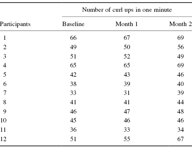
2. A physical education teacher conducted an action research project to examine a strength and conditioning program. Using 12 male participants, she measures the number of curl ups they could do in 1 min. She measured their performance before the programs. Then, she measured their performance at 1 month intervals. Table 5.10 presents the performance results.
Use a Friedman test with α = 0.05 to determine if one or more of the groups are significantly different. The teacher is expecting performance gains, so if a significant difference exists, use one-tailed Wilcoxon signed rank tests to identify which groups are significantly different. Use the Bonferroni procedure to limit the type I error rate. Report your findings.
5.7 Solutions to Practice Questions
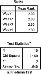
1. The results from the Friedman test are displayed in SPSS Output 5.2.
According to the data, the results from the Friedman test indicated that the four conditions were not significantly different (Fr(3) = 2.160, p > 0.10). Therefore, no follow-up contrasts are needed.
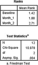
2. The results from the Friedman test are displayed in SPSS Output 5.3a.
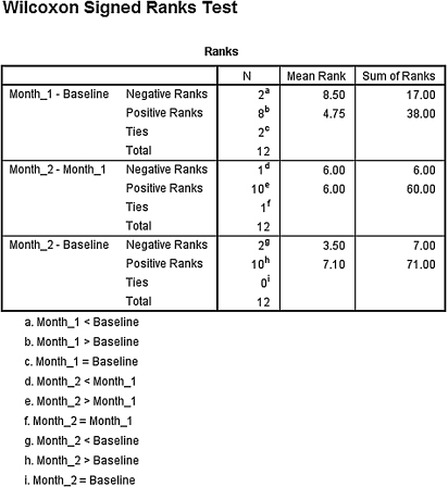
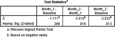
According to the data, the results from the Friedman test indicated that one or more of the three groups are significantly different (Fr(2) = 10.978, p < 0.05). Therefore, we must examine each set of samples with follow-up contrasts to find the differences between groups. We compare the samples with Wilcoxon signed rank tests. Since there are k = 3 groups, use αB = 0.0167 to avoid type I error rate inflation. The results from the Wilcoxon signed rank tests are displayed in SPSS Outputs 5.4 and 5.5.
- Baseline–Month 1 Comparison. The results from the Wilcoxon signed rank test (T = 17.0, n = 12, p > 0.0167) indicated that the two samples were not significantly different.
- Month 1–Month 2 Comparison. The results from the Wilcoxon signed rank test (T = 6.0, n = 12, p < 0.0167) indicated that the two samples were significantly different.
- Baseline–Month 2 Comparison. The results from the Wilcoxon signed rank test (T = 7.0, n = 12, p < 0.0167) indicated that the two samples were significantly different.