CHAPTER 6
Comparing More Than Two Unrelated Samples: The Kruskal–Wallis H-Test
6.1 Objectives
In this chapter, you will learn the following items.
- How to compute the Kruskal–Wallis H-test.
- How to perform contrasts to compare samples.
- How to perform the Kruskal–Wallis H-test and associated sample contrasts using SPSS®.
6.2 Introduction
A professor asked her students to complete end-of-course evaluations for her Psychology 101 class. She taught four sections of the course and wants to compare the evaluation results from each section. Since the evaluations were based on a five-point rating scale, she decides to use a nonparametric procedure. Moreover, she recognizes that the four sets of evaluation results are independent or unrelated. In other words, no single score in any single class is dependent on any other score in any other class. This professor could compare her sections using the Kruskal–Wallis H-test.
The Kruskal–Wallis H-test is a nonparametric statistical procedure for comparing more than two samples that are independent or not related. The parametric equivalent to this test is the one-way analysis of variance (ANOVA).
When the Kruskal–Wallis H-test leads to significant results, then at least one of the samples is different from the other samples. However, the test does not identify where the difference(s) occurs. Moreover, it does not identify how many differences occur. In order to identify the particular differences between sample pairs, a researcher might use sample contrasts, or post hoc tests, to analyze the specific sample pairs for significant difference(s). The Mann–Whitney U-test is a useful method for performing sample contrasts between individual sample sets.
In this chapter, we will describe how to perform and interpret a Kruskal–Wallis H-test followed with sample contrasts. We will also explain how to perform the procedures using SPSS. Finally, we offer varied examples of these nonparametric statistics from the literature.
6.3 Computing The Kruskal–Wallis H-Test Statistic
The Kruskal–Wallis H-test is used to compare more than two independent samples. When stating our hypotheses, we state them in terms of the population. Moreover, we examine the population medians, θi, when performing the Kruskal–Wallis H-test.
To compute the Kruskal–Wallis H-test statistic, we begin by combining all of the samples and rank ordering the values together. Use Formula 6.1 to determine an H statistic:
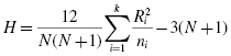
where N is the number of values from all combined samples, Ri is the sum of the ranks from a particular sample, and ni is the number of values from the corresponding rank sum.
The degrees of freedom, df, for the Kruskal–Wallis H-test are determined by using Formula 6.2:
where df is the degrees of freedom and k is the number of groups.
Once the test statistic H is computed, it can be compared with a table of critical values (see Table B.6 in Appendix B) to examine the groups for significant differences. However, if the number of groups, k, or the numbers of values in each sample, ni, exceed those available from the table, then a large sample approximation may be performed. Use a table with the χ2 distribution (see Table B.2 in Appendix B) to obtain a critical value when performing a large sample approximation.
If ranking of values results in any ties, a tie correction is required. In that case, find a new H statistic by dividing the original H statistic by the tie correction. Use Formula 6.3 to determine the tie correction value;
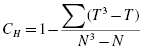
where CH is the ties correction, T is the number of values from a set of ties, and N is the number of values from all combined samples.
If the H statistic is not significant, then no differences exist between any of the samples. However, if the H statistic is significant, then a difference exists between at least two of the samples. Therefore, a researcher might use sample contrasts between individual sample pairs, or post hoc tests, to determine which of the sample pairs are significantly different.
When performing multiple sample contrasts, the type I error rate tends to become inflated. Therefore, the initial level of risk, or α, must be adjusted. We demonstrate the Bonferroni procedure, shown in Formula 6.4, to adjust α:
where αB is the adjusted level of risk, α is the original level of risk, and k is the number of comparisons.
6.3.1 Sample Kruskal–Wallis H-Test (Small Data Samples)
Researchers were interested in studying the social interaction of different adults. They sought to determine if social interaction can be tied to self-confidence. The researchers classified 17 participants into three groups based on the social interaction exhibited. The participant groups were labeled as follows:
- High = constant interaction; talks with many different people; initiates discussion
- Medium = interacts with a variety of people; some periods of isolation; tends to focus on fewer people
- Low = remains mostly isolated from others; speaks if spoken to, but leaves interaction quickly
After the participants had been classified into the three social interaction groups, they were directed to complete a self-assessment of self-confidence on a 25-point scale. Table 6.1 shows the scores obtained by each of the participants, with 25 points being an indication of high self-confidence.
| Original ordinal self-confidence scores placed within social interaction groups | ||
|---|---|---|
| High | Medium | Low |
| 21 | 19 | 7 |
| 23 | 5 | 8 |
| 18 | 10 | 15 |
| 12 | 11 | 3 |
| 19 | 9 | 6 |
| 20 | 4 | |
The original survey scores obtained were converted to an ordinal scale prior to the data analysis. Table 6.1 shows the ordinal values placed in the social interaction groups.
We want to determine if there is a difference between any of the three groups in Table 6.1. Since the data belong to an ordinal scale and the sample sizes are small (n < 20), we will use a nonparametric test. The Kruskal–Wallis H-test is a good choice to analyze the data and test the hypothesis.
6.3.1.1 State the Null and Research Hypotheses
The null hypothesis states that there is no tendency for self-confidence to rank systematically higher or lower for any of the levels of social interaction. The research hypothesis states that there is a tendency for self-confidence to rank systematically higher or lower for at least one level of social interaction than at least one of the other levels. We generally use the concept of “systematic differences” in the hypotheses.
The null hypothesis is
HO: θL = θM = θH
The research hypothesis is
HA: There is a tendency for self-confidence to rank systematically higher or lower for at least one level of social interaction when compared with the other levels.
6.3.1.2 Set the Level of Risk (or the Level of Significance) Associated with the Null Hypothesis
The level of risk, also called an alpha (α), is frequently set at 0.05. We will use α = 0.05 in our example. In other words, there is a 95% chance that any observed statistical difference will be real and not due to chance.
6.3.1.3 Choose the Appropriate Test Statistic
The data are obtained from three independent, or unrelated, samples of adults who are being assigned to three different social interaction groups by observation. They are then being assessed using a self-confidence scale with a total of 25 points. The three samples are small with some violations of our assumptions of normality. Since we are comparing three independent samples, we will use the Kruskal–Wallis H-test.
6.3.1.4 Compute the Test Statistic
First, combine and rank the three samples together (see Table 6.2).
| Original ordinal score | Participant rank | Social interaction group |
|---|---|---|
| 3 | 1 | Low |
| 4 | 2 | Low |
| 5 | 3 | Medium |
| 6 | 4 | Low |
| 7 | 5 | Low |
| 8 | 6 | Low |
| 9 | 7 | Medium |
| 10 | 8 | Medium |
| 11 | 9 | Medium |
| 12 | 10 | High |
| 15 | 11 | Low |
| 18 | 12 | High |
| 19 | 13.5 | Medium |
| 19 | 13.5 | High |
| 20 | 15 | High |
| 21 | 16 | High |
| 23 | 17 | High |
Place the participant ranks in their social interaction groups to compute the sum of ranks Ri for each group (see Table 6.3).
Next, compute the sum of ranks for each social interaction group. The ranks in each group are added to obtain a total R-value for the group.
For the high group,
For the medium group,
For the low group,
These R-values are used to compute the Kruskal–Wallis H-test statistic (see Formula 6.1). The number of participants in each group is identified by a lowercase n. The total group size in the study is identified by the uppercase N.
Now, using the data from Table 6.3, compute the H-test statistic using Formula 6.1:

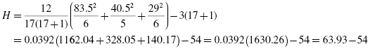
Since there was a tie involved in the ranking, correct the value of H. First, compute the tie correction (see Formula 6.2). Then, divide the original H statistic by the ties correction CH:
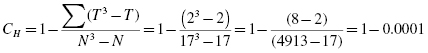
Next, we divide to find the corrected H statistic:
For this set of data, notice that the corrected H does not differ greatly from the original H. With the correction, H = 9.94.
6.3.1.5 Determine the Value Needed for Rejection of the Null Hypothesis Using the Appropriate Table of Critical Values for the Particular Statistic
We will use the critical value table for the Kruskal–Wallis H-test (see Table B.6 in Appendix B) since it includes the number of groups, k, and the numbers of samples, n, for our data. In this case, we look for the critical value for k = 3 and n1 = 6, n2 = 6, and n3 = 5 with α = 0.05. Table B.5 returns a critical value for the Kruskal–Wallis H-test of 5.76.
6.3.1.6 Compare the Obtained Value with the Critical Value
The critical value for rejecting the null hypothesis is 5.76 and the obtained value is H = 9.94. If the critical value is less than or equal to the obtained value, we must reject the null hypothesis. If instead, the critical value exceeds the obtained value, we do not reject the null hypothesis. Since critical value is less than the obtained value, we must reject the null hypothesis.
At this point, it is worth mentioning that larger samples often result in more ties. While comparatively small, as observed in step 4, corrections for ties can make a difference in the decision regarding the null hypothesis. If the H were near the critical value of 5.99 for df = 2 (e.g., H = 5.80), and the tie correction calculated to be 0.965, the decision would be to reject the null hypothesis with the correction (H = 6.01), but to not reject the null hypothesis without the correction. Therefore, it is important to perform tie corrections.
6.3.1.7 Interpret the Results
We rejected the null hypothesis, suggesting that a real difference in self-confidence exists between one or more of the three social interaction types. In particular, the data show that those who were classified as fitting the definition of the “low” group were mostly people who reported poor self-confidence, and those who were in the “high” group were mostly people who reported good self-confidence. However, describing specific differences in this manner is speculative. Therefore, we need a technique for statistically identifying difference between groups, or contrasts.
Sample Contrasts, or Post Hoc Tests
The Kruskal–Wallis H-test identifies if a statistical difference exists; however, it does not identify how many differences exist and which samples are different. To identify which samples are different and which are not, we can use a procedure called contrasts or post hoc tests. Methods for comparing two samples at a time are described in Chapters 3 and 4. The examples in this chapter compare unrelated samples so we will use the Mann–Whitney U-test.
It is important to note that performing several two-sample tests has a tendency to inflate the type I error rate. In our example, we would compare three groups, k = 3. At α = 0.05, the type I error rate would be 1 − (1 − 0.05)3 = 0.14.
To compensate for this error inflation, we demonstrate the Bonferroni procedure (see Formula 6.4). With this technique, we use a corrected α with the Mann–Whitney U-tests to determine significant differences between samples. For our example,
When we compare each set of samples with the Mann–Whitney U-tests and use αB, we obtain the following results presented in Table 6.4.
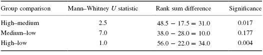
Since αB = 0.0167, we notice that the high–low group comparison is indeed significantly different. The medium–low group comparison is not significant. The high–medium group comparison requires some judgment since it is difficult to tell if the difference is significant or not; the way the value is rounded off could change the result.
Note that if you are not comparing all of the samples for the Kruskal–Wallis H-test, then k is only the number of comparisons you are making with the Mann–Whitney U-tests. Therefore, comparing fewer samples will increase the chances of finding a significant difference.
6.3.1.8 Reporting the Results
The reporting of results for the Kruskal–Wallis H-test should include such information as sample size for all of the groups, the H statistic, degrees of freedom, and p-value's relation to α. For this example, three social interaction groups were compared: high (nH = 6), medium (nM = 5), and low (nL = 6). The Kruskal–Wallis H-test was significant (H(2) = 9.94, p < 0.05). In order to compare each set of samples, contrasts may be used as described earlier in this chapter.
6.3.2 Performing the Kruskal–Wallis H-Test Using SPSS
We will analyze the data from the example earlier using SPSS.
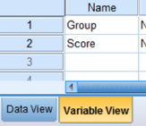
6.3.2.1 Define Your Variables
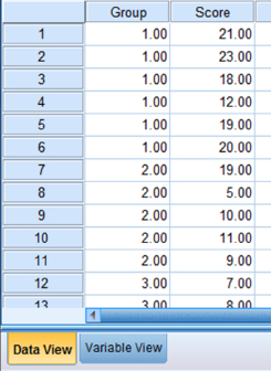
First, click the “Variable View” tab at the bottom of your screen. Then, type the names of your variables in the “Name” column. Unlike the Friedman's ANOVA described in Chapter 5, you cannot simply enter each sample into a separate column to execute the Kruskal–Wallis H-test. You must use a grouping variable. In Figure 6.1, the first variable is the grouping variable that we called “Group.” The second variable that we called “Score” will have our actual values.
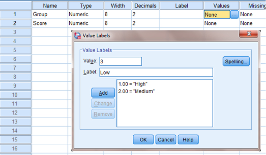
When establishing a grouping variable, it is often easiest to assign each group a whole number value. In our example, our groups are “High,” “Medium,” and “Low.” Therefore, we must set our grouping variables for the variable “Group.” First, we selected the “Values” column and clicked the gray square as shown in Figure 6.2. Then, we set a value of 1 to equal “High,” a value of 2 to equal “Medium,” and a value of 3 equal to “Low.” Each value label is established and moved to the list when we click the “Add” button. Once we click the “OK” button, we are returned to the SPSS Variable View.
6.3.2.2 Type in Your Values
Click the “Data View” tab at the bottom of your screen as shown in Figure 6.3. Type in the values for all three samples in the “Score” column. As you do so, type in the corresponding grouping variable in the “Group” column. For example, all of the values for “High” are signified by a value of 1 in the grouping variable column that we called “Group.”
6.3.2.3 Analyze Your Data
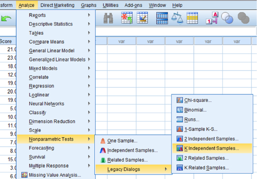
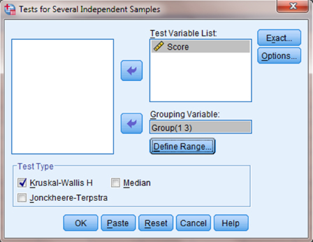
As shown in Figure 6.4, use the pull-down menus to choose “Analyze,” “Nonparametric Tests,” “Legacy Dialogs,” and “K Independent Samples. …”
Use the top arrow button to place your variable with your data values, or dependent variable (DV), in the box labeled “Test Variable List:.” Then, use the lower arrow button to place your grouping variable, or independent variable (IV), in the box labeled “Grouping Variable.” As shown in Figure 6.5, we have placed the “Score” variable in the “Test Variable List” and the “Group” variable in the “Grouping Variable” box.
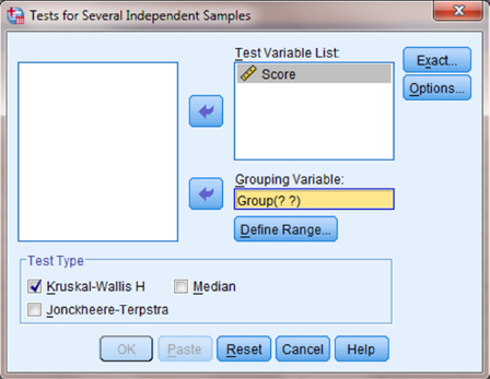
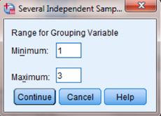
Click on the “Define Range …” button to assign a reference value to your independent variable (i.e., “Grouping Variable”).
As shown in Figure 6.6, type 1 into the box next to “Minimum” and 3 in the box next to “Maximum.” Then, click “Continue.” This step references the value labels you defined when you established your grouping variable.
Now that the groups have been assigned (see Fig. 6.7), click “OK” to perform the analysis.
6.3.2.4 Interpret the Results from the SPSS Output Window
SPSS Output 6.1 provides the mean ranks of groups and group sizes. The second output table provides the Kruskal–Wallis H-test statistic (H = 9.944). Since this test uses a χ2 distribution, SPSS calls the H statistic “Chi-Square.” This table also returns the degrees of freedom (df = 2) and the significance (p = 0.007).
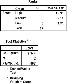
Based on the results from SPSS, three social interaction groups were compared: high (nH = 6), medium (nM = 5), and low (nL = 6). The Kruskal–Wallis H-test was significant (H(2) = 9.94, p < 0.05). In order to compare individual pairs of samples, contrasts must be used.
Note that to perform Mann–Whitney U-tests for sample contrasts, simply use the grouping values you established when you defined your variables in step 1. Remember to use your corrected level of risk αB when examining your significance.
6.3.3 Sample Kruskal–Wallis H-Test (Large Data Samples)
Researchers were interested in continuing their study of social interaction. In a new study, they examined the self-confidence of teenagers with respect to social interaction. Three levels of social interaction were based on the following characteristics:
- High = constant interaction; talks with many different people; initiates discussion
- Medium = interacts with a variety of people; some periods of isolation; tends to focus on fewer people
- Low = remains mostly isolated from others; speaks if spoken to, but leaves interaction quickly
The researchers assigned each participant into one of the three social interaction groups. Researchers administered a self-assessment of self-confidence. The assessment instrument measured self-confidence on a 50-point ordinal scale. Table 6.5 shows the scores obtained by each of the participants, with 50 points indicating high self-confidence.
| Original self-confidence scores placed within social interaction groups | ||
|---|---|---|
| High | Medium | Low |
| 18 | 35 | 37 |
| 27 | 47 | 24 |
| 24 | 11 | 7 |
| 30 | 31 | 19 |
| 48 | 12 | 20 |
| 16 | 39 | 14 |
| 43 | 11 | 38 |
| 46 | 14 | 16 |
| 49 | 40 | 12 |
| 34 | 48 | 31 |
| 28 | 32 | 15 |
| 20 | 9 | 20 |
| 37 | 44 | 25 |
| 21 | 30 | 10 |
| 20 | 33 | 36 |
| 16 | 26 | 45 |
| 23 | 22 | 48 |
| 12 | 3 | 42 |
| 50 | 41 | 42 |
| 25 | 17 | 21 |
| 8 | ||
| 10 | ||
| 41 | ||
We want to determine if there is a difference between any of the three groups in Table 6.5. The Kruskal–Wallis H-test will be used to analyze the data.
6.3.3.1 State the Null and Research Hypotheses
The null hypothesis states that there is no tendency for teen self-confidence to rank systematically higher or lower for any of the levels of social interaction. The research hypothesis states that there is a tendency for teen self-confidence to rank systematically higher or lower for at least one level of social interaction than at least one of the other levels. We generally use the concept of “systematic differences” in the hypotheses.
The null hypothesis is
HO: θL = θM = θH
The research hypothesis is
HA: There is a tendency for teen self-confidence to rank systematically higher or lower for at least one level of social interaction when compared with the other levels.
6.3.3.2 Set the Level of Risk (or the Level of Significance) Associated with the Null Hypothesis
The level of risk, also called an alpha (α), is frequently set at 0.05. We will use α = 0.05 in our example. In other words, there is a 95% chance that any observed statistical difference will be real and not due to chance.
6.3.3.3 Choose the Appropriate Test Statistic
The data are obtained from three independent, or unrelated, samples of teenagers. They were assessed using an instrument with a 50-point ordinal scale. Since we are comparing three independent samples of values based on an ordinal scale instrument, we will use the Kruskal–Wallis H-test.
6.3.3.4 Compute the Test Statistic
First, combine and rank the three samples together (see Table 6.6).
| Original ordinal score | Participant rank | Social interaction group |
|---|---|---|
| 3 | 1 | Medium |
| 7 | 2 | Low |
| 8 | 3 | Medium |
| 9 | 4 | Medium |
| 10 | 5.5 | Medium |
| 10 | 5.5 | Low |
| 11 | 7.5 | Medium |
| 11 | 7.5 | Medium |
| 12 | 10 | High |
| 12 | 10 | Medium |
| 12 | 10 | Low |
| 14 | 12.5 | Medium |
| 14 | 12.5 | Low |
| 15 | 14 | Low |
| 16 | 16 | High |
| 16 | 16 | High |
| 16 | 16 | Low |
| 17 | 18 | Medium |
| 18 | 19 | High |
| 19 | 20 | Low |
| 20 | 22.5 | High |
| 20 | 22.5 | High |
| 20 | 22.5 | Low |
| 20 | 22.5 | Low |
| 21 | 25.5 | High |
| 21 | 25.5 | Low |
| 22 | 27 | Medium |
| 23 | 28 | High |
| 24 | 29.5 | High |
| 24 | 29.5 | Low |
| 25 | 31.5 | High |
| 25 | 31.5 | Low |
| 26 | 33 | Medium |
| 27 | 34 | High |
| 28 | 35 | High |
| 30 | 36.5 | High |
| 30 | 36.5 | Medium |
| 31 | 38.5 | Medium |
| 31 | 38.5 | Low |
| 32 | 40 | Medium |
| 33 | 41 | Medium |
| 34 | 42 | High |
| 35 | 43 | Medium |
| 36 | 44 | Low |
| 37 | 45.5 | High |
| 37 | 45.5 | Low |
| 38 | 47 | Low |
| 39 | 48 | Medium |
| 40 | 49 | Medium |
| 41 | 50.5 | Medium |
| 41 | 50.5 | Medium |
| 42 | 52.5 | Low |
| 42 | 52.5 | Low |
| 43 | 54 | High |
| 44 | 55 | Medium |
| 45 | 56 | Low |
| 46 | 57 | High |
| 47 | 58 | Medium |
| 48 | 60 | High |
| 48 | 60 | Medium |
| 48 | 60 | Low |
| 49 | 62 | High |
| 50 | 63 | High |
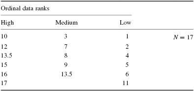
Place the participant ranks in their social interaction groups to compute the sum of ranks, Ri, for each group (see Table 6.7).
| Ordinal data ranks | ||
|---|---|---|
| High | Medium | Low |
| 10 | 1 | 2 |
| 16 | 3 | 5.5 |
| 16 | 4 | 10 |
| 19 | 5.5 | 12.5 |
| 22.5 | 7.5 | 14 |
| 22.5 | 7.5 | 16 |
| 25.5 | 10 | 20 |
| 28 | 12.5 | 22.5 |
| 29.5 | 18 | 22.5 |
| 31.5 | 27 | 25.5 |
| 34 | 33 | 29.5 |
| 35 | 36.5 | 31.5 |
| 36.5 | 38.5 | 38.5 |
| 42 | 40 | 44 |
| 45.5 | 41 | 45.5 |
| 54 | 43 | 47 |
| 57 | 48 | 52.5 |
| 60 | 49 | 52.5 |
| 62 | 50.5 | 56 |
| 63 | 50.5 | 60 |
| 55 | ||
| 58 | ||
| 60 | ||
Next, compute the sum of ranks for each social interaction group. The ranks in each group are added to obtain a total R-value for the group.
- For the high group, RH = 709.5 and nH = 20.
- For the medium group, RM = 699 and nM = 23.
- For the low group, RL = 607.5 and nL = 20.
These R-values are used to compute the Kruskal–Wallis H-test statistic (see Formula 6.1). The number of participants in each group is identified by a lowercase n. The total group size in the study is identified by the uppercase N. In this study, N = 63.
Now, using the data from Table 6.7, compute the H statistic using Formula 6.1:

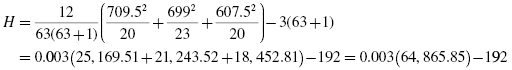
Since there were ties involved in the ranking, correct the value of H. First, compute the tie correction (see Formula 6.2). There were 11 sets of ties with two values, three sets of ties with three values, and one set of ties with four values. Then, divide the original H statistic by the tie correction CH:
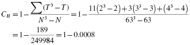
Next, we divide to find the corrected H statistic:
For this set of data, notice that the corrected H does not differ greatly from the original H. With the correction, H = 1.054.
6.3.3.5 Determine the Value Needed for Rejection of the Null Hypothesis Using the Appropriate Table of Critical Values for the Particular Statistic
Since the data have at least one large sample, we will use the χ2 distribution (see Table B.2 found in Appendix B) to find the critical value for the Kruskal–Wallis H-test. In this case, we look for the critical value for df = 2 and α = 0.05. Using the table, the critical value for rejecting the null hypothesis is 5.99.
6.3.3.6 Compare the Obtained Value with the Critical Value
The critical value for rejecting the null hypothesis is 5.99 and the obtained value is H = 1.054. If the critical value is less than or equal to the obtained value, we must reject the null hypothesis. If instead, the critical value exceeds the obtained value, we do not reject the null hypothesis. Since the critical value exceeds the obtained value, we do not reject the null hypothesis.
6.3.3.7 Interpret the Results
We did not reject the null hypothesis, suggesting that no real difference exists between any of the three groups. In particular, the data suggest that there is no difference in self-confidence between one or more of the three social interaction types.
6.3.3.8 Reporting the Results
The reporting of results for the Kruskal–Wallis H-test should include such information as sample size for each of the groups, the H statistic, degrees of freedom, and p-value's relation to α. For this example, three social interaction groups were compared. The three social interaction groups were high (nH = 20), medium (nM = 23), and low (nL = 20). The Kruskal–Wallis H-test was not significant (H(2) = 1.054, p < 0.05).
6.4 Examples from the Literature
To be shown are varied examples of the nonparametric procedures described in this chapter. We have summarized each study's research problem and researchers' rationale(s) for choosing a nonparametric approach. We encourage you to obtain these studies if you are interested in their results.
Gömleksız and Bulut (2007) examined primary school teachers' views on the implementation and effectiveness of a new primary school mathematics curriculum. When they examined the data, some of the samples were found to be non-normal. For those samples, they used a Kruskal–Wallis H-test, followed by Mann–Whitney U-tests to compare unrelated samples.
In the study of Finson et al. (2006), the students of nine middle school teachers were asked to draw a scientist. Based on the drawings, students' perceptions of scientists were compared with their teachers' teaching styles using the Kruskal–Wallis H-test. Then, the samples were individually compared using Mann–Whitney U-test. The researchers used nonparametric statistical analyses because only relatively small sample sizes of subjects were available.
Belanger and Desrochers (2001) investigated the nature of infants' ability to perceive event causality. The researchers noted that they chose nonparametric statistical tests because the data samples lacked a normal distribution based on results from a Shapiro–Wilk test. In addition, they stated that the sample sizes were small. A Kruskal–Wallis H-test revealed no significant differences between samples. Therefore, they did not perform any sample contrasts.
Plata and Trusty (2005) investigated the willingness of high school boys' willingness to allow same-sex peers with learning disabilities (LDs) to participate in school activities and out-of-school activities. The authors compared the willingness of 38 educationally successful and 33 educationally at-risk boys. The boys were from varying socioeconomic backgrounds. Due to the data's ordinal nature and small sample sizes among some samples, nonparametric statistics were used for the analysis. The Kruskal–Wallis H-test was chosen for multiple comparisons. When sample pairs were compared, the researchers performed a post-hoc analysis of the differences between mean rank pairs using a multiple comparison technique.
6.5 Summary
More than two samples that are not related may be compared using a nonparametric procedure called the Kruskal–Wallis H-test. The parametric equivalent to this test is known as the one-way analysis of variance (ANOVA). When the Kruskal–Wallis H-test produces significant results, it does not identify which nor how many sample pairs are significantly different. The Mann–Whitney U-test, with a Bonferroni procedure to avoid type I error rate inflation, is a useful method for comparing individual sample pairs.
In this chapter, we described how to perform and interpret a Kruskal–Wallis H-test followed with sample contrasts. We also explained how to perform the procedures using SPSS. Finally, we offered varied examples of these nonparametric statistics from the literature. The next chapter will involve comparing two variables.
6.6 Practice Questions
1. A researcher conducted a study with n = 15 participants to investigate strength gains from exercise. The participants were divided into three groups and given one of three treatments. Participants' strength gains were measured and ranked. The rankings are presented in Table 6.8.
Use a Kruskal–Wallis H-test with α = 0.05 to determine if one or more of the groups are significantly different. If a significant difference exists, use a two-tailed Mann–Whitney U-tests or two-sample Kolmogorov–Smirnov tests to identify which groups are significantly different. Use the Bonferroni procedure to limit the type I error rate. Report your findings.
2. A researcher investigated how physical attraction influences the perception among others of a person's effectiveness with difficult tasks. The photographs of 24 people were shown to a focus group. The group was asked to classify the photos into three groups: very attractive, average, and very unattractive. Then, the group ranked the photographs according to their impression of how capable they were of solving difficult problems. Table 6.9 shows the classification and rankings of the people in the photos (1 = most effective, 24 = least effective).
Use a Kruskal–Wallis H-test with α = 0.05 to determine if one or more of the groups are significantly different. If a significant difference exists, use two-tailed Mann–Whitney U-tests to identify which groups are significantly different. Use the Bonferroni procedure to limit the type I error rate. Report your findings.
| Treatments | ||
|---|---|---|
| I | II | III |
| 7 | 13 | 12 |
| 2 | 1 | 5 |
| 4 | 7 | 16 |
| 11 | 8 | 9 |
| 15 | 3 | 14 |
| Very attractive | Average | Very unattractive |
|---|---|---|
| 1 | 3 | 11 |
| 2 | 4 | 15 |
| 5 | 8 | 16 |
| 6 | 9 | 18 |
| 7 | 13 | 20 |
| 10 | 14 | 21 |
| 12 | 19 | 23 |
| 17 | 22 | 24 |
6.7 Solutions to Practice Questions
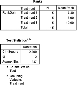
1. The results from the Kruskal–Wallis H-test are displayed in SPSS Output 6.2.
According to the data, the results from the Kruskal–Wallis H-test indicated that the three groups are not significantly different (H(2) = 2.800, p > 0.05). Therefore, no follow-up contrasts are needed.
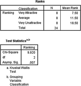
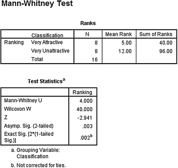
2. The results from the Kruskal–Wallis H-test are displayed in SPSS Output 6.3.
According to the data, the results from the Kruskal–Wallis H-test indicated that one or more of the three groups are significantly different (H(2) = 9.920, p < 0.05). Therefore, we must examine each set of samples with follow-up contrasts to find the differences between groups.
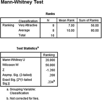
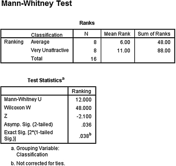
Based on the significance from the Kruskal–Wallis H-test, we compare the samples with Mann–Whitney U-tests. Since there are k = 3 groups, use αB = 0.0167 to avoid type I error rate inflation. The results from the Mann–Whitney U-tests are displayed in the remaining SPSS Output 6.4, SPSS Output 6.5, and SPSS Output 6.6.
- Very Attractive–Attractive Comparison.
The results from the Mann–Whitney U-test (U = 20.0, n1 = 8, n2 = 8, p > 0.0167) indicated that the two samples were not significantly different. - Attractive–Very Unattractive Comparison.
The results from the Mann–Whitney U-test (U = 12.0, n1 = 8, n2 = 8, p > 0.0167) indicated that the two samples were not significantly different. - Very Attractive–Very Unattractive Comparison.
The results from the Mann–Whitney U-test (U = 4.0, n1 = 8, n2 = 8, p < 0.0167) indicated that the two samples were significantly different.