CHAPTER 7
Comparing Variables of Ordinal or Dichotomous Scales: Spearman Rank-Order, Point-Biserial, and Biserial Correlations
7.1 Objectives
In this chapter, you will learn the following items:
- How to compute the Spearman rank-order correlation coefficient.
- How to perform the Spearman rank-order correlation using SPSS®.
- How to compute the point-biserial correlation coefficient.
- How to perform the point-biserial correlation using SPSS.
- How to compute the biserial correlation coefficient.
7.2 Introduction
The statistical procedures in this chapter are quite different from those in the last several chapters. Unlike this chapter, we had compared samples of data. This chapter, however, examines the relationship between two variables. In other words, this chapter will address how one variable changes with respect to another.
The relationship between two variables can be compared with a correlation analysis. If any of the variables are ordinal or dichotomous, we can use a nonparametric correlation. The Spearman rank-order correlation, also called the Spearman's ρ, is used to compare the relationship between ordinal, or rank-ordered, variables. The point-biserial and biserial correlations are used to compare the relationship between two variables if one of the variables is dichotomous. The parametric equivalent to these correlations is the Pearson product-moment correlation.
In this chapter, we will describe how to perform and interpret a Spearman rank-order, point-biserial, and biserial correlations. We will also explain how to perform the procedures using SPSS. Finally, we offer varied examples of these nonparametric statistics from the literature.
7.3 The Correlation Coefficient
When comparing two variables, we use an obtained value called a correlation coefficient. A population's correlation coefficient is represented by the Greek letter rho, ρ. A sample's correlation coefficient is represented by the letter r.
We will describe two types of relationships between variables. A direct relationship is a positive correlation with an obtained value ranging from 0 to 1.0. As one variable increases, the other variable also increases. An indirect, or inverse, relationship is a negative correlation with an obtained value ranging from 0 to −1.0. In this case, one variable increases as the other variable decreases.
In general, a significant correlation coefficient also communicates the relative strength of a relationship between the two variables. A value close to 1.0 or −1.0 indicates a nearly perfect relationship, while a value close to 0 indicates an especially weak or trivial relationship. Cohen (1988, 1992) presented a more detailed description of a correlation coefficient's relative strength. Table 7.1 summarizes his findings.
| Correlation coefficient for a direct relationship | Correlation coefficient for an indirect relationship | Relationship strength of the variables |
|---|---|---|
| 0.0 | 0.0 | None/trivial |
| 0.1 | −0.1 | Weak/small |
| 0.3 | −0.3 | Moderate/medium |
| 0.5 | −0.5 | Strong/large |
| 1.0 | −1.0 | Perfect |
There are three important caveats to consider when assigning relative strength to correlation coefficients, however. First, Cohen's work was largely based on behavioral science research. Therefore, these values may be inappropriate in fields such as engineering or the natural sciences. Second, the correlation strength assignments vary for different types of statistical tests. Third, r-values are not based on a linear scale. For example, r = 0.6 is not twice as strong as r = 0.3.
7.4 Computing the Spearman Rank-Order Correlation Coefficient
The Spearman rank-order correlation is a statistical procedure that is designed to measure the relationship between two variables on an ordinal scale of measurement if the sample size is n ≥ 4. Use Formula 7.1 to determine a Spearman rank-order correlation coefficient rs if none of the ranked values are ties. Sometimes, the symbol rs is represented by the Greek symbol rho, or ρ:
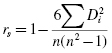
where n is the number of rank pairs and Di is the difference between a ranked pair.
If ties are present in the values, use Formula 7.2, Formula 7.3, and Formula 7.4 to determine rs:
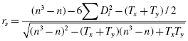
where
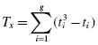
and
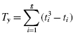
g is the number of tied groups in that variable and ti is the number of tied values in a tie group.
If there are no ties in a variable, then T = 0.
Use Formula 7.5 to determine the degrees of freedom for the correlation:
where n is the number of paired values.
After rs is determined, it must be examined for significance. Small samples allow one to reference a table of critical values, such as Table B.7 found in Appendix B. However, if the sample size n exceeds those available from the table, then a large sample approximation may be performed. For large samples, compute a z-score and use a table with the normal distribution (see Table B.1 in Appendix B) to obtain a critical region of z-scores. Formula 7.6 may be used to find the z-score of a correlation coefficient for large samples:
where n is the number of paired values and r is the correlation coefficient.
Note that the method for determining a z-score given a correlation coefficient and examining it for significance is the same for each type of correlation. We will illustrate a large sample approximation with a sample problem when we address the point-biserial correlation.
Although we will use Formula 7.6 to determine the significance of the correlation coefficient, some statisticians recommend using the formula based on the Student's t-distribution, as shown in Formula 7.7:
According to Siegel and Castellan (1988), the advantage of using the Student's t-distribution over the z-score is small with larger sample sizes n.
7.4.1 Sample Spearman Rank-Order Correlation (Small Data Samples without Ties)
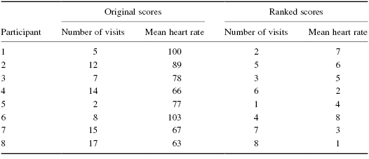
Eight men were involved in a study to examine the resting heart rate regarding frequency of visits to the gym. The assumption is that the person who visits the gym more frequently for a workout will have a slower heart rate. Table 7.2 shows the number of visits each participant made to the gym during the month the study was conducted. It also provides the mean heart rate measured at the end of the week during the final 3 weeks of the month.
| Participant | Number of visits | Mean heart rate |
|---|---|---|
| 1 | 5 | 100 |
| 2 | 12 | 89 |
| 3 | 7 | 78 |
| 4 | 14 | 66 |
| 5 | 2 | 77 |
| 6 | 8 | 103 |
| 7 | 15 | 67 |
| 8 | 17 | 63 |
The values in this study do not possess characteristics of a strong interval scale. For instance, the number of visits to the gym does not necessarily communicate duration and intensity of physical activity. In addition, heart rate has several factors that can result in differences from one person to another. Ordinal measures offer a clearer relationship to compare these values from one individual to the next. Therefore, we will convert these values to ranks and use a Spearman rank-order correlation.
7.4.1.1 State the Null and Research Hypothesis
The null hypothesis states that there is no correlation between number of visits to the gym in a month and mean resting heart rate. The research hypothesis states that there is a correlation between the number of visits to the gym and the mean resting heart rate.
The null hypothesis is
HO: ρs = 0
The research hypothesis is
HA: ρs ≠ 0
7.4.1.2 Set the Level of Risk (or the Level of Significance) Associated with the Null Hypothesis
The level of risk, also called an alpha (α), is frequently set at 0.05. We will use α = 0.05 in our example. In other words, there is a 95% chance that any observed statistical difference will be real and not due to chance.
7.4.1.3 Choose the Appropriate Test Statistic
As stated earlier, we decided to analyze the variables using an ordinal, or rank, procedure. Therefore, we will convert the values in each variable to ordinal data. In addition, we will be comparing the two variables, the number of visits to the gym in a month and the mean resting heart rate. Since we are comparing two variables in which one or both are measured on an ordinal scale, we will use the Spearman rank-order correlation.
7.4.1.4 Compute the Test Statistic
First, rank the scores for each variable separately as shown in Table 7.3. Rank them from the lowest score to the highest score to form an ordinal distribution for each variable.
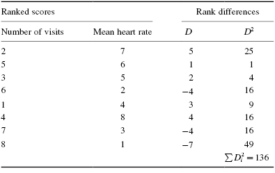
To calculate the Spearman rank-order correlation coefficient, we need to calculate the differences between rank pairs and their subsequent squares where D = rank (mean heart rate) − rank (number of visits). It is helpful to organize the data to manage the summation in the formula (see Table 7.4).
Next, compute the Spearman rank-order correlation coefficient:
7.4.1.5 Determine the Value Needed for Rejection of the Null Hypothesis Using the Appropriate Table of Critical Values for the Particular Statistic
Table B.7 in Appendix B lists critical values for the Spearman rank-order correlation coefficient. In this study, the critical value is found for n = 8 and df = 6. Since we are conducting a two-tailed test and α = 0.05, the critical value is 0.738. If the obtained value exceeds or is equal to the critical value, 0.738, we will reject the null hypothesis. If the critical value exceeds the absolute value of the obtained value, we will not reject the null hypothesis.
7.4.1.6 Compare the Obtained Value with the Critical Value
The critical value for rejecting the null hypothesis is 0.738 and the obtained value is |rs| = 0.619. If the critical value is less than or equal to the obtained value, we must reject the null hypothesis. If instead, the critical value is greater than the obtained value, we must not reject the null hypothesis. Since the critical value exceeds the absolute value of the obtained value, we do not reject the null hypothesis.
7.4.1.7 Interpret the Results
We did not reject the null hypothesis, suggesting that there is no significant correlation between the number of visits the males made to the gym in a month and their mean resting heart rates.
7.4.1.8 Reporting the Results
The reporting of results for the Spearman rank-order correlation should include such information as the number of participants (n), two variables that are being correlated, correlation coefficient (rs), degrees of freedom (df), and p-value's relation to α.
For this example, eight men (n = 8) were observed for 1 month. Their number of visits to the gym was documented (variable 1) and their mean resting heart rate was recorded during the last 3 weeks of the month (variable 2). These data were put in ordinal form for purposes of the analysis. The Spearman rank-order correlation coefficient was not significant (rs(6) = −0.619, p > 0.05). Based on this data, we can state that there is no clear relationship between adult male resting heart rate and the frequency of visits to the gym.
7.4.2 Sample Spearman Rank-Order Correlation (Small Data Samples with Ties)
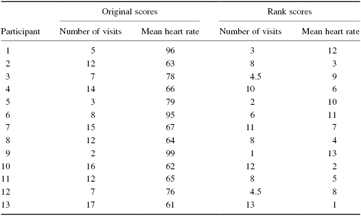
The researcher repeated the experiment in the previous example using females. Table 7.5 shows the number of visits each participant made to the gym during the month of the study and their subsequent mean heart rates.
| Participant | Number of visits | Mean heart rate |
|---|---|---|
| 1 | 5 | 96 |
| 2 | 12 | 63 |
| 3 | 7 | 78 |
| 4 | 14 | 66 |
| 5 | 3 | 79 |
| 6 | 8 | 95 |
| 7 | 15 | 67 |
| 8 | 12 | 64 |
| 9 | 2 | 99 |
| 10 | 16 | 62 |
| 11 | 12 | 65 |
| 12 | 7 | 76 |
| 13 | 17 | 61 |
As with the previous example, the values in this study do not possess characteristics of a strong interval scale, so we will use ordinal measures. We will convert these values to ranks and use a Spearman rank-order correlation.
Steps 1–3 are the same as the previous example. Therefore, we will begin with step 4.
7.4.2.1 Compute the Test Statistic
First, rank the scores for each variable as shown in Table 7.6. Rank the scores from the lowest score to the highest score to form an ordinal distribution for each variable.
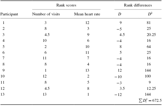
To calculate the Spearman rank-order correlation coefficient, we need to calculate the differences between rank pairs and their subsequent squares where D = rank (mean heart rate) − rank (number of visits). It is helpful to organize the data to manage the summation in the formula (see Table 7.7).
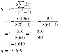
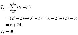
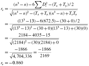
Next, compute the Spearman rank-order correlation coefficient. Since there are ties present in the ranks, we will use formulas that account for the ties. First, use Formula 7.3 and Formula 7.4. For the number of visits, there are two groups of ties. The first group has two tied values (rank = 4.5 and t = 2) and the second group has three tied values (rank = 8 and t = 3):
For the mean resting heart rate, there are no ties. Therefore, Ty = 0. Now, calculate the Spearman rank-order correlation coefficient using Formula 7.2:
7.4.2.2 Determine the Value Needed for Rejection of the Null Hypothesis Using the Appropriate Table of Critical Values for the Particular Statistic
Table B.7 in Appendix B lists critical values for the Spearman rank-order correlation coefficient. To be significant, the absolute value of the obtained value, |rs|, must be greater than or equal to the critical value on the table. In this study, the critical value is found for n = 13 and df = 11. Since we are conducting a two-tailed test and α = 0.05, the critical value is 0.560.
7.4.2.3 Compare the Obtained Value with the Critical Value
The critical value for rejecting the null hypothesis is 0.560 and the obtained value is |rs| = 0.860. If the critical value is less than or equal to the obtained value, we must reject the null hypothesis. If instead, the critical value is greater than the obtained value, we must not reject the null hypothesis. Since the critical value is less than the absolute value of the obtained value, we reject the null hypothesis.
7.4.2.4 Interpret the Results
We rejected the null hypothesis, suggesting that there is a significant correlation between the number of visits the females made to the gym in a month and their mean resting heart rates.
7.4.2.5 Reporting the Results
The reporting of results for the Spearman rank-order correlation should include such information as the number of participants (n), two variables that are being correlated, correlation coefficient (rs), degrees of freedom (df), and p-value's relation to α.
For this example, 13 women (n = 13) were observed for 1 month. Their number of visits to the gym was documented (variable 1) and their mean resting heart rate was recorded during the last 3 weeks of the month (variable 2). These data were put in ordinal form for purposes of the analysis. The Spearman rank-order correlation coefficient was significant (rs(11) = −0.860, p < 0.05). Based on this data, we can state that there is a very strong inverse relationship between adult female resting heart rate and the frequency of visits to the gym.
7.4.3 Performing the Spearman Rank-Order Correlation Using SPSS
We will analyze the data from the previous example using SPSS.
7.4.3.1 Define Your Variables
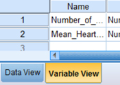
First, click the “Variable View” tab at the bottom of your screen. Then, type the names of your variables in the “Name” column. As shown in Figure 7.1, the first variable is called “Number_of_Visits” and the second variable is called “Mean_Heart_Rate.”
7.4.3.2 Type in Your Values
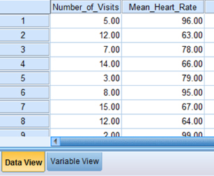
Click the “Data View” tab at the bottom of your screen as shown in Figure 7.2. Type the values in the respective columns.
7.4.3.3 Analyze Your Data
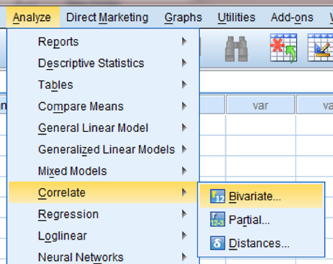
As shown in Figure 7.3, use the pull-down menus to choose “Analyze,” “Correlate,” and “Bivariate… .”
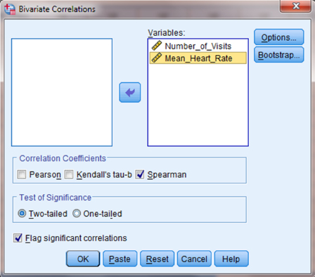
Use the arrow button to place both variables with your data values in the box labeled “Variables:” as shown in Figure 7.4. Then, in the “Correlation Coefficients” box, uncheck “Pearson” and check “Spearman.” Finally, click “OK” to perform the analysis.
7.4.3.4 Interpret the Results from the SPSS Output Window
The output table (see SPSS Output 7.1) provides the Spearman rank-order correlation coefficient (rs = −0.860) labeled Spearman's rho. It also returns the number of pairs (n = 13) and the two-tailed significance (p ≈ 0.000). In this example, the significance is not actually zero. The reported value does not return enough digits to show the significance's actual precision.
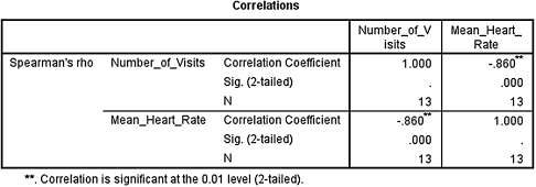
Based on the results from SPSS, the Spearman rank-order correlation coefficient was significant (rs(11) = −0.860, p < 0.05). Based on these data, we can state that there is a very strong inverse relationship between adult female resting heart rate and the frequency of visits to the gym.
7.5 Computing the Point-Biserial and Biserial Correlation Coefficients
The point-biserial and biserial correlations are statistical procedures for use with dichotomous variables. A dichotomous variable is simply a measure of two conditions. A dichotomous variable is either discrete or continuous. A discrete dichotomous variable has no particular order and might include such examples as gender (male vs. female) or a coin toss (heads vs. tails). A continuous dichotomous variable has some type of order to the two conditions and might include measurements such as pass/fail or young/old. Finally, since the point-biserial and biserial correlations each involves an interval scale analysis, they are special cases of the Pearson product-moment correlation.
7.5.1 Correlation of a Dichotomous Variable and an Interval Scale Variable
The point-biserial correlation is a statistical procedure to measure the relationship between a discrete dichotomous variable and an interval scale variable. Use Formula 7.8 to determine the point-biserial correlation coefficient rpb:
where ![]() is the mean of the interval variable's values associated with the dichotomous variable's first category,
is the mean of the interval variable's values associated with the dichotomous variable's first category, ![]() is the mean of the interval variable's values associated with the dichotomous variable's second category, s is the standard deviation of the variable on the interval scale, Pp is the proportion of the interval variable values associated with the dichotomous variable's first category, and Pq is the proportion of the interval variable values associated with the dichotomous variable's second category.
is the mean of the interval variable's values associated with the dichotomous variable's second category, s is the standard deviation of the variable on the interval scale, Pp is the proportion of the interval variable values associated with the dichotomous variable's first category, and Pq is the proportion of the interval variable values associated with the dichotomous variable's second category.
Recall the formulas for mean (Formula 7.9) and standard deviation (Formula 7.10):
and
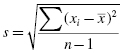
where ![]() is the sum of the values in the sample and n is the number of values in the sample.
is the sum of the values in the sample and n is the number of values in the sample.
The biserial correlation is a statistical procedure to measure the relationship between a continuous dichotomous variable and an interval scale variable. Use Formula 7.11 to determine the biserial correlation coefficient rb:
where ![]() is the mean of the interval variable's values associated with the dichotomous variable's first category,
is the mean of the interval variable's values associated with the dichotomous variable's first category, ![]() is the mean of the interval variable's values associated with the dichotomous variable's second category, sx is the standard deviation of the variable on the interval scale, Pp is the proportion of the interval variable values associated with the dichotomous variable's first category, Pq is the proportion of the interval variable values associated with the dichotomous variable's second category, and y is the height of the unit normal curve ordinate at the point dividing Pp and Pq (see Fig. 7.5).
is the mean of the interval variable's values associated with the dichotomous variable's second category, sx is the standard deviation of the variable on the interval scale, Pp is the proportion of the interval variable values associated with the dichotomous variable's first category, Pq is the proportion of the interval variable values associated with the dichotomous variable's second category, and y is the height of the unit normal curve ordinate at the point dividing Pp and Pq (see Fig. 7.5).
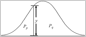
You may use Table B.1 in Appendix B or Formula 7.12 to find the height of the unit normal curve ordinate, y:
where e is the natural log base and approximately equal to 2.718282 and z is the z-score at the point dividing Pp and Pq.
Formula 7.13 is the relationship between the point-biserial and the biserial correlation coefficients. This formula is necessary to find the biserial correlation coefficient because SPSS only determines the point-biserial correlation coefficient:
After the correlation coefficient is determined, it must be examined for significance. Small samples allow one to reference a table of critical values, such as Table B.8 found in Appendix B. However, if the sample size n exceeds those available from the table, then a large sample approximation may be performed. For large samples, compute a z-score and use a table with the normal distribution (see Table B.1 in Appendix B) to obtain a critical region of z-scores. As described earlier in this chapter, Formula 7.6 may be used to find the z-score of a correlation coefficient for large samples.
7.5.2 Correlation of a Dichotomous Variable and a Rank-Order Variable
As explained earlier, the point-biserial and biserial correlation procedures earlier involve a dichotomous variable and an interval scale variable. If the correlation was a dichotomous variable and a rank-order variable, a slightly different approach is needed.
To find the point-biserial correlation coefficient for a discrete dichotomous variable and a rank-order variable, simply use the Spearman rank-order described earlier and assign arbitrary values to the dichotomous variable such as 0 and 1. To find the biserial correlation coefficient for a continuous dichotomous variable and a rank-order variable, use the same procedure and then apply Formula 7.13 given earlier.
7.5.3 Sample Point-Biserial Correlation (Small Data Samples)
A researcher in a psychological lab investigated gender differences. She wished to compare male and female ability to recognize and remember visual details. She used 17 participants (8 males and 9 females) who were initially unaware of the actual experiment. First, she placed each one of them alone in a room with various objects and asked them to wait. After 10 min, she asked each of the participants to complete a 30 question posttest relating to several details in the room. Table 7.8 shows the participants' genders and posttest scores.
| Participant | Gender | Posttest score |
|---|---|---|
| 1 | M | 7 |
| 2 | M | 19 |
| 3 | M | 8 |
| 4 | M | 10 |
| 5 | M | 7 |
| 6 | M | 15 |
| 7 | M | 6 |
| 8 | M | 13 |
| 9 | F | 14 |
| 10 | F | 11 |
| 11 | F | 18 |
| 12 | F | 23 |
| 13 | F | 17 |
| 14 | F | 20 |
| 15 | F | 14 |
| 16 | F | 24 |
| 17 | F | 22 |
The researcher wishes to determine if a relationship exists between the two variables and the relative strength of the relationship. Gender is a discrete dichotomous variable and visual detail recognition is an interval scale variable. Therefore, we will use a point-biserial correlation.
7.5.3.1 State the Null and Research Hypothesis
The null hypothesis states that there is no correlation between gender and visual detail recognition. The research hypothesis states that there is a correlation between gender and visual detail recognition.
The null hypothesis is
HO: ρpb = 0
The research hypothesis is
HA: ρpb ≠ 0
7.5.3.2 Set the Level of Risk (or the Level of Significance) Associated with the Null Hypothesis
The level of risk, also called an alpha (α), is frequently set at 0.05. We will use α = 0.05 in our example. In other words, there is a 95% chance that any observed statistical difference will be real and not due to chance.
7.5.3.3 Choose the Appropriate Test Statistic
As stated earlier, we decided to analyze the relationship between the two variables. A correlation will provide the relative strength of the relationship between the two variables. Gender is a discrete dichotomous variable and visual detail recognition is an interval scale variable. Therefore, we will use a point-biserial correlation.
7.5.3.4 Compute the Test Statistic
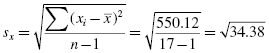
First, compute the standard deviation of all values from the interval scale data. It is helpful to organize the data as shown in Table 7.9.
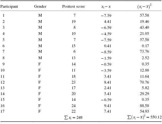
Using the summations from Table 7.9, calculate the mean and the standard deviation for the interval data:
Next, compute the means and proportions of the values associated with each item from the dichotomous variable. The mean males' posttest score was
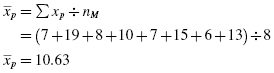
The mean females' posttest score was

The males' proportion was

The females' proportion was

Now, compute the point-biserial correlation coefficient using the values computed earlier:
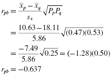
The sign on the correlation coefficient is dependent on the order we managed our dichotomous variable. Since that was arbitrary, the sign is irrelevant. Therefore, we use the absolute value of the point-biserial correlation coefficient:
7.5.3.5 Determine the Value Needed for Rejection of the Null Hypothesis Using the Appropriate Table of Critical Values for the Particular Statistic
Table B.8 in Appendix B lists critical values for the Pearson product-moment correlation coefficient. Using the critical values, table requires that the degrees of freedom be known. Since df = n − 2 and n = 17, then df = 17 − 2. Therefore, df = 15. Since we are conducting a two-tailed test and α = 0.05, the critical value is 0.482.
7.5.3.6 Compare the Obtained Value with the Critical Value
The critical value for rejecting the null hypothesis is 0.482 and the obtained value is |rpb| = 0.637. If the critical value is less than or equal to the obtained value, we must reject the null hypothesis. If instead, the critical value is greater than the obtained value, we must not reject the null hypothesis. Since the critical value is less than the absolute value of the obtained value, we reject the null hypothesis.
7.5.3.7 Interpret the Results
We rejected the null hypothesis, suggesting that there is a significant and moderately strong correlation between gender and visual detail recognition.
7.5.3.8 Reporting the Results
The reporting of results for the point-biserial correlation should include such information as the number of participants (n), two variables that are being correlated, correlation coefficient (rpb), degrees of freedom (df), p-value's relation to α, and the mean values of each dichotomous variable.
For this example, a researcher compared male and female ability to recognize and remember visual details. Eight males (nM = 8) and nine females (nF = 9) participated in the experiment. The researcher measured participants' visual detail recognition with a 30 question test requiring participants to recall details in a room they had occupied. A point-biserial correlation produced significant results (rpb(15) = 0.637, p < 0.05). These data suggest that there is a strong relationship between gender and visual detail recognition. Moreover, the mean scores on the detail recognition test indicate that males (![]() ) recalled fewer details, while females (
) recalled fewer details, while females (![]() ) recalled more details.
) recalled more details.
7.5.4 Performing the Point-Biserial Correlation Using SPSS
We will analyze the data from the previous example using SPSS.
7.5.4.1 Define Your Variables
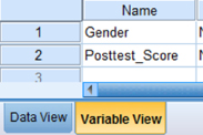
First, click the “Variable View” tab at the bottom of your screen. Then, type the names of your variables in the “Name” column. As shown in Figure 7.6, the first variable is called “Gender” and the second variable is called “Posttest_Score.”
7.5.4.2 Type in Your Values
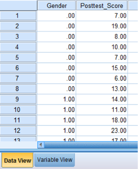
Click the “Data View” tab at the bottom of your screen as shown in Figure 7.7. Type in the values in the respective columns. Gender is a discrete dichotomous variable and SPSS needs a code to reference the values. We code male values with 0 and female values with 1. Any two values can be chosen for coding the data.
7.5.4.3 Analyze Your Data
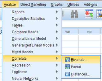
As shown in Figure 7.8, use the pull-down menus to choose “Analyze,” “Correlate,” and “Bivariate… .”
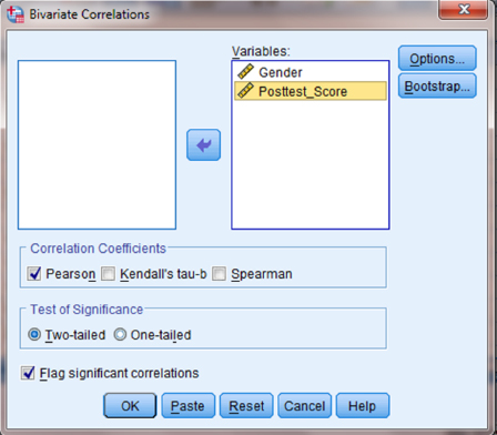
Use the arrow button near the middle of the window to place both variables with your data values in the box labeled “Variables:” as shown in Figure 7.9. In the “Correlation Coefficients” box, “Pearson” should remain checked since the Pearson product-moment correlation will perform an approximate point-biserial correlation. Finally, click “OK” to perform the analysis.
7.5.4.4 Interpret the Results from the SPSS Output Window
The output table (see SPSS Output 7.2) provides the Pearson product-moment correlation coefficient (r = 0.657). This correlation coefficient is approximately equal to the point-biserial correlation coefficient. It also returns the number of pairs (n = 17) and the two-tailed significance (p = 0.004).
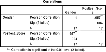
Based on the results from SPSS, the point-biserial correlation coefficient was significant (rpb(15) = 0.657, p < 0.05). Based on these data, we can state that there is a strong relationship between gender and visual detail recognition (as measured by the posttest).
7.5.5 Sample Point-Biserial Correlation (Large Data Samples)
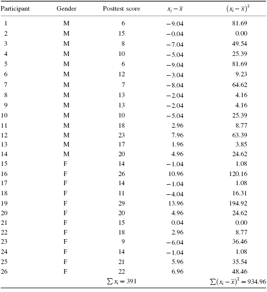
A colleague of the researcher from the previous example wished to replicate the study investigating gender differences. As before, he compared male and female ability to recognize and remember visual details. He used 26 participants (14 males and 12 females) who were initially unaware of the actual experiment. Table 7.10 shows the participants' genders and posttest scores.
| Participant | Gender | Posttest score |
|---|---|---|
| 1 | M | 6 |
| 2 | M | 15 |
| 3 | M | 8 |
| 4 | M | 10 |
| 5 | M | 6 |
| 6 | M | 12 |
| 7 | M | 7 |
| 8 | M | 13 |
| 9 | M | 13 |
| 10 | M | 10 |
| 11 | M | 18 |
| 12 | M | 23 |
| 13 | M | 17 |
| 14 | M | 20 |
| 15 | F | 14 |
| 16 | F | 26 |
| 17 | F | 14 |
| 18 | F | 11 |
| 19 | F | 29 |
| 20 | F | 20 |
| 21 | F | 15 |
| 22 | F | 18 |
| 23 | F | 9 |
| 24 | F | 14 |
| 25 | F | 21 |
| 26 | F | 22 |
We will once again use a point-biserial correlation. However, we will use a large sample approximation to examine the results for significance since the sample size is large.
7.5.5.1 State the Null and Research Hypothesis
The null hypothesis states that there is no correlation between gender and visual detail recognition. The research hypothesis states that there is a correlation between gender and visual detail recognition.
The null hypothesis is
HO: ρpb = 0
The research hypothesis is
HA: ρpb ≠ 0
7.5.5.2 Set the Level of Risk (or the Level of Significance) Associated with the Null Hypothesis
The level of risk, also called an alpha (α), is frequently set at 0.05. We will use α = 0.05 in our example. In other words, there is a 95% chance that any observed statistical difference will be real and not due to chance.
7.5.5.3 Choose the Appropriate Test Statistic
As stated earlier, we decided to analyze the relationship between the two variables. A correlation will provide the relative strength of the relationship between the two variables. Gender is a discrete dichotomous variable and visual detail recognition is an interval scale variable. Therefore, we will use a point-biserial correlation.
7.5.5.4 Compute the Test Statistic
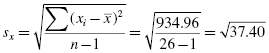
First, compute the standard deviation of all values from the interval scale data. Organize the data to manage the summations (see Table 7.11):
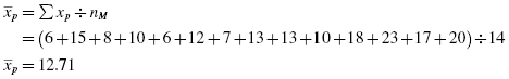
Next, compute the means and proportions of the values associated with each item from the dichotomous variable. The mean males' posttest score was
The mean females' posttest score was
The males' proportion was

The females' proportion was

Now, compute the point-biserial correlation coefficient using the values computed earlier:
The sign on the correlation coefficient is dependent on the order we managed our dichotomous variable. Since that was arbitrary, the sign is irrelevant. Therefore, we use the absolute value of the point-biserial correlation coefficient:
Since our number of values is large, we will use a large sample approximation to examine the obtained value for significance. We will find a z-score for our data using an approximation to the normal distribution:
7.5.5.5 Determine the Value Needed for Rejection of the Null Hypothesis Using the Appropriate Table of Critical Values for the Particular Statistic
Table B.1 in Appendix B is used to establish the critical region of z-scores. For a two-tailed test with α = 0.05, we must not reject the null hypothesis if −1.96 ≤ z* ≤ 1.96.
7.5.5.6 Compare the Obtained Value with the Critical Value
Notice that z* is in the positive tail of the distribution (2.055 > 1.96). Therefore, we reject the null hypothesis. This suggests that the correlation between gender and visual detail recognition is real.
7.5.5.7 Interpret the Results
We rejected the null hypothesis, suggesting that there is a significant and moderately weak correlation between gender and visual detail recognition.
7.5.5.8 Reporting the Results
The reporting of results for the point-biserial correlation should include such information as the number of participants (n), two variables that are being correlated, correlation coefficient (rpb), degrees of freedom (df), p-value's relation to α, and the mean values of each dichotomous variable.
For this example, a researcher replicated a study that compared male and female ability to recognize and remember visual details. Fourteen males (nM = 14) and 12 females (nF = 12) participated in the experiment. The researcher measured participants' visual detail recognition with a 30 question test requiring participants to recall details in a room they had occupied. A point-biserial correlation produced significant results (rpb(24) = 0.411, p < 0.05). These data suggest that there is a moderate relationship between gender and visual detail recognition. Moreover, the mean scores on the detail recognition test indicate that males (![]() ) recalled fewer details, while females (
) recalled fewer details, while females (![]() ) recalled more details.
) recalled more details.
7.5.6 Sample Biserial Correlation (Small Data Samples)
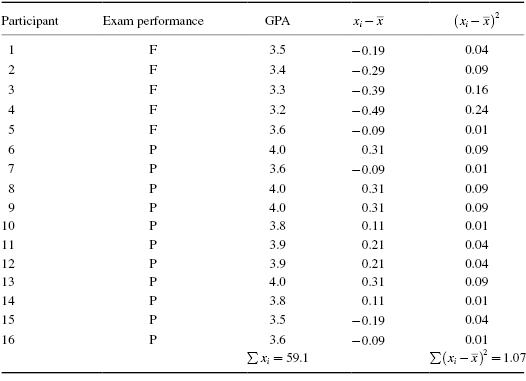
A graduate anthropology department at a university wished to determine if its students' grade point averages (GPAs) can be used to predict performance on the department's comprehensive exam required for graduation. The comprehensive exam is graded on a pass/fail basis. Sixteen students participated in the comprehensive exam last year. Five of the students failed the exam. The GPAs and the exam performance of the students are displayed in Table 7.12.
| Participant | Exam performance | GPA |
|---|---|---|
| 1 | F | 3.5 |
| 2 | F | 3.4 |
| 3 | F | 3.3 |
| 4 | F | 3.2 |
| 5 | F | 3.6 |
| 6 | P | 4.0 |
| 7 | P | 3.6 |
| 8 | P | 4.0 |
| 9 | P | 4.0 |
| 10 | P | 3.8 |
| 11 | P | 3.9 |
| 12 | P | 3.9 |
| 13 | P | 4.0 |
| 14 | P | 3.8 |
| 15 | P | 3.5 |
| 16 | P | 3.6 |
Exam performance is a continuous dichotomous variable and GPA is an interval scale variable. Therefore, we will use a biserial correlation.
7.5.6.1 State the Null and Research Hypothesis
The null hypothesis states that there is no correlation between student GPA and comprehensive exam performance. The research hypothesis states that there is a correlation between student GPA and comprehensive exam performance.
The null hypothesis is
HO: ρb = 0
The research hypothesis is
HA: ρb ≠ 0
7.5.6.2 Set the Level of Risk (or the Level of Significance) Associated with the Null Hypothesis
The level of risk, also called an alpha (α), is frequently set at 0.05. We will use α = 0.05 in our example. In other words, there is a 95% chance that any observed statistical difference will be real and not due to chance.
7.5.6.3 Choose the Appropriate Test Statistic
As stated earlier, we decided to analyze the relationship between the two variables. A correlation will provide the relative strength of the relationship between the two variables. Exam performance is a continuous dichotomous variable and GPA is an interval scale variable. Therefore, we will use a biserial correlation.
7.5.6.4 Compute the Test Statistic
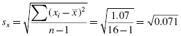
First, compute the standard deviation of all values from the interval scale data. Organize the data to manage the summations (see Table 7.13):
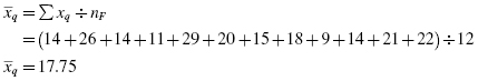
Next, compute the means and proportions of the values associated with each item from the dichotomous variable. The mean GPA of the exam failures was
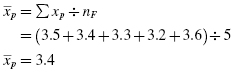
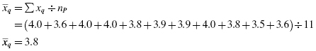
The mean GPA of the ones who passed the exam was
The proportion of exam failures was

The proportion of the ones who passed the exam was

Now, determine the height of the unit normal curve ordinate, y, at the point dividing Pp and Pq. We could reference the table of values for the normal distribution, such as Table B.1 in Appendix B, to find y. However, we will compute the value. Using Table B.1 also provides the z-score at the point dividing Pp and Pq, z = 0.49:
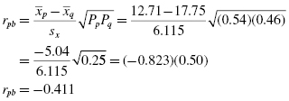
Now, compute the biserial correlation coefficient using the values computed earlier:
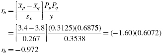
The sign on the correlation coefficient is dependent on the order we managed our dichotomous variable. A quick inspection of the variable means indicates that the GPA of the failures was smaller than the GPA of the ones who passed. Therefore, we should convert the biserial correlation coefficient to a positive value:
7.5.6.5 Determine the Value Needed for Rejection of the Null Hypothesis Using the Appropriate Table of Critical Values for the Particular Statistic
Table B.8 in Appendix B lists critical values for the Pearson product-moment correlation coefficient. The table requires the degrees of freedom and df = n − 2. In this study, n = 16 and df = 16 − 2. Therefore, df = 14. Since we are conducting a two-tailed test and α = 0.05, the critical value is 0.497.
7.5.6.6 Compare the Obtained Value with the Critical Value
The critical value for rejecting the null hypothesis is 0.497 and the obtained value is |rb| = 0.972. If the critical value is less than or equal to the obtained value, we must reject the null hypothesis. If instead, the critical value is greater than the obtained value, we must not reject the null hypothesis. Since the critical value is less than the absolute value of the obtained value, we reject the null hypothesis.
7.5.6.7 Interpret the Results
We rejected the null hypothesis, suggesting that there is a significant and very strong correlation between student GPA and comprehensive exam performance.
7.5.6.8 Reporting the Results
The reporting of results for the biserial correlation should include such information as the number of participants (n), two variables that are being correlated, correlation coefficient (rb), degrees of freedom (df), p-value's relation to α, and the mean values of each dichotomous variable.
For this example, a researcher compared the GPAs of graduate anthropology students who passed their comprehensive exam with students who failed the exam. Five students failed the exam (nF = 5) and 11 students passed it (nP = 11). The researcher compared student GPA and comprehensive exam performance. A biserial correlation produced significant results (rb(14) = 0.972, p < 0.05). The data suggest that there is an especially strong relationship between student GPA and comprehensive exam performance. Moreover, the mean GPA of the failing students (![]() ) and passing students (
) and passing students (![]() ) indicates that the relationship is a direct correlation.
) indicates that the relationship is a direct correlation.
7.5.7 Performing the Biserial Correlation Using SPSS
SPSS does not compute the biserial correlation coefficient. To do so, Field (2005) has suggested using SPSS to perform a Pearson product-moment correlation (as described earlier) and then applying Formula 7.13. However, this procedure will only produce an approximation of the biserial correlation coefficient and we recommend you use a spreadsheet with the procedure we described for the sample biserial correlation.
7.6 Examples from the Literature
Listed are varied examples of the nonparametric procedures described in this chapter. We have summarized each study's research problem and researchers' rationale(s) for choosing a nonparametric approach. We encourage you to obtain these studies if you are interested in their results.
Greiner and Smith (2006) investigated factors that might affect teacher retention. When they examined the relationship between the Texas state-mandated teacher certification examination and teacher retention, they used a point-biserial correlation. The researchers used the point biserial since teacher retention was measured as a discrete dichotomous variable.
Blumberg and Sokol (2004) examined gender differences in the cognitive strategies that 2nd- and 5th-grade children use when they learn how to play a video game. In part of the study, participants were classified as frequent players or infrequent players. That classification was correlated with game performance. Since player frequency was a discrete dichotomy, the researchers chose a point-biserial correlation.
McMillian et al. (2006) investigated the attitudes of female registered nurses toward male registered nurses. The researchers performed several analyses with a variety of statistical tests. In one analysis, they used a Spearman rank-order correlation to examine the relationship between town population and the participants' responses on an attitude inventory. The attitude inventory was a modified instrument to measure level of sexist attitude. Participants indicated agreement or disagreement with statements using a four-point Likert scale. The Spearman rank-order correlation was chosen because the attitude inventory resembled an ordinal scale.
Fitzgerald et al (2007) examined the validity of an instrument designed to measure the performance of physical therapy interns. They used a correlation analysis to examine the relationship between two measures of clinical competence. Since one of the measures was ordinal, the researchers used a Spearman rank-order correlation.
Flannelly et al. (2005) reviewed the research literature of studies that investigated the effects of religion on adolescent tobacco use. The authors used a biserial correlation to compare studies' effect (no effect vs. effect) with sample size.
7.7 Summary
The relationship between two variables can be compared with a correlation analysis. If any of the variables are ordinal or dichotomous, a nonparametric correlation is useful. The Spearman rank-order correlation, also called the Spearman's ρ, is used to compare the relationship involving ordinal, or rank-ordered, variables. The point-biserial and biserial correlations are used to compare the relationship between two variables if one of the variables is dichotomous. The parametric equivalent to these correlations is the Pearson product-moment correlation.
In this chapter, we described how to perform and interpret a Spearman rank-order, point-biserial, and biserial correlations. We also explained how to perform the procedures using SPSS. Finally, we offered varied examples of these nonparametric statistics from the literature. The next chapter will involve comparing nominal scale data.
7.8 Practice Questions
1. The business department at a small college wanted to compare the relative class rank of its MBA graduates with their fifth-year salaries. The data collected by the department are presented in Table 7.14. Compare the graduates' class rank with their fifth-year salaries.
Use a two-tailed Spearman rank-order correlation with α = 0.05 to determine if a relationship exists between the two variables. Report your findings.
2. A researcher was contracted by the military to assess soldiers' perception of a new training program's effectiveness. Fifteen soldiers participated in the program. The researcher used a survey to measure the soldiers' perceptions of the program's effectiveness. The survey used a Likert-type scale that ranged from 5 = strongly agree to 1 = strongly disagree. Using the data presented in Table 7.15, compare the soldiers' average survey scores with the total number of years the soldiers had been serving.
Use a two-tailed Spearman rank-order correlation with α = 0.05 to determine if a relationship exists between the two variables. Report your findings.
3. A middle school history teacher wished to determine if there is a connection between gender and history knowledge among 8th-grade gifted students. The teacher administered a 50 item test at the beginning of the school year to 16 gifted 8th-grade students. The scores from the test are presented in Table 7.16.
Use a two-tailed point-biserial correlation with α = 0.05 to determine if a relationship exists between the two variables. Report your findings.
4. A researcher wished to determine if there is a connection between poverty and self-esteem. Income level was used to classify 18 participants as either below poverty or above poverty. Participants completed a 20 item survey to measure self-esteem. The scores from the survey are reported in Table 7.17.
Use a two-tailed biserial correlation with α = 0.05 to determine if a relationship exists between the two variables. Report your findings.
| Relative class rank | Fifth-year salary ($) |
|---|---|
| 1 | 83,450 |
| 2 | 67,900 |
| 3 | 89,000 |
| 4 | 80,500 |
| 5 | 91,000 |
| 6 | 55,440 |
| 7 | 101,300 |
| 8 | 50,560 |
| 9 | 76,050 |
| Average survey score | Years of service |
|---|---|
| 4.0 | 18 |
| 4.0 | 15 |
| 2.4 | 2 |
| 4.2 | 13 |
| 3.4 | 4 |
| 4.0 | 10 |
| 5.0 | 24 |
| 1.8 | 4 |
| 3.2 | 9 |
| 2.5 | 5 |
| 2.5 | 3 |
| 3.0 | 8 |
| 3.6 | 16 |
| 4.6 | 14 |
| 4.8 | 12 |
| Participant | Gender | Posttest score |
|---|---|---|
| 1 | M | 44 |
| 2 | M | 30 |
| 3 | M | 50 |
| 4 | M | 33 |
| 5 | M | 37 |
| 6 | M | 35 |
| 7 | M | 36 |
| 8 | F | 29 |
| 9 | F | 39 |
| 10 | F | 33 |
| 11 | F | 50 |
| 12 | F | 45 |
| 13 | F | 37 |
| 14 | F | 30 |
| 15 | F | 34 |
| 16 | F | 50 |
| Participant | Poverty level | Survey score |
|---|---|---|
| 1 | Above | 15 |
| 2 | Above | 19 |
| 3 | Above | 15 |
| 4 | Above | 20 |
| 5 | Above | 7 |
| 6 | Above | 12 |
| 7 | Above | 3 |
| 8 | Above | 15 |
| 9 | Below | 9 |
| 10 | Below | 5 |
| 11 | Below | 13 |
| 12 | Below | 13 |
| 13 | Below | 11 |
| 14 | Below | 10 |
| 15 | Below | 8 |
| 16 | Below | 9 |
| 17 | Below | 10 |
| 18 | Below | 17 |
7.9 Solutions to Practice Questions
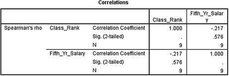
1. The results from the analysis are displayed in SPSS Output 7.3.
The results from the Spearman rank-order correlation (rs = −0.217, p > 0.05) did not produce significant results. Based on these data, we can state that there is no clear relationship between graduates' relative class rank and fifth-year salary.
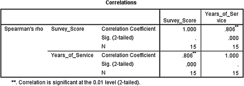
2. The results from the analysis are displayed in SPSS Output 7.4.
The results from the Spearman rank-order correlation (rs = 0.806, p < 0.05) produced significant results. Based on these data, we can state that there is a very strong correlation between soldiers' survey scores concerning the new program's effectiveness and their total years of military service.
3. The results from the point-biserial correlation (rpb = 0.047, p > 0.05) did not produce significant results. Based on these data, we can state that there is no clear relationship between 8th-grade gifted students' gender and their score on the history knowledge test administered by the teacher.
Note that the results obtained from using SPSS is rpb = 0.049, p > 0.05.
4. The results from the biserial correlation (rb = 0.372, p > 0.05) did not produce significant results. Based on these data, we can state that there is no clear relationship between poverty level and self-esteem.